Normal distribution. We say that a random variable X follows the normal distribution if the probability density function of X is given by

Transcription

1 Normal distribution The normal distribution is the most important distribution. It describes well the distribution of random variables that arise in practice, such as the heights or weights of people, the total annual sales of a firm, exam scores etc. Also, it is important for the central limit theorem, the approximation of other distributions such as the binomial, etc. We say that a random variable X follows the normal distribution if the probability density function of X is given by f(x) = 1 σ 1 2π e 2 ( x µ This is a bell-shaped curve. σ )2, < x < We write X N(µ, σ). We read: X follows the normal distribution (or X is normally distributed) with mean µ, and standard deviation σ. The normal distribution can be described completely by the two parameters µ and σ. As always, the mean is the center of the distribution and the standard deviation is the measure of the variation around the mean. Shape of the normal distribution. Suppose X N(5, 2). X ~ N(5,2) f(x) x The area under the normal curve is 1 (100%). 1 σ 2π e 1 2 ( x µ σ )2 dx = 1 The normal distribution is symmetric about µ. Therefore, the area to the left of µ is equal to the area to the right of µ (50% each). 1

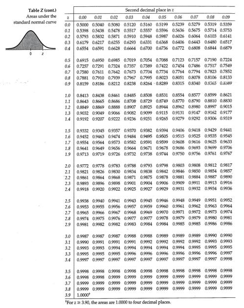
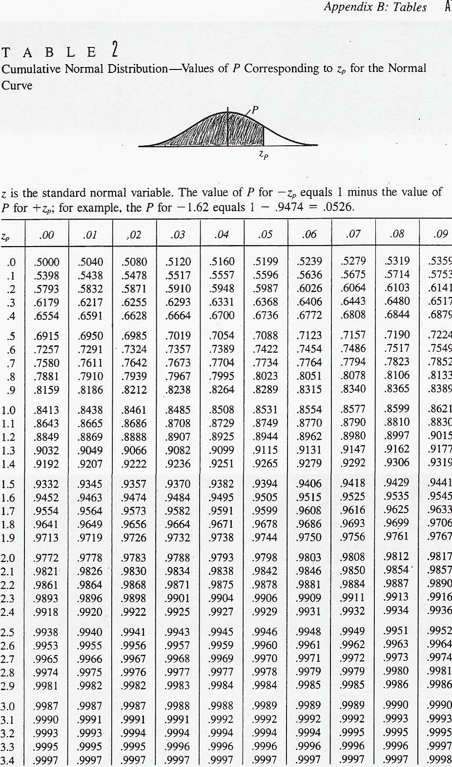
2 Useful rule (see figure above): The interval µ ± 1σ covers the middle 68% of the distribution. The interval µ ± 2σ covers the middle 95% of the distribution. The interval µ ± 3σ covers the middle 100% of the distribution. Because the normal distribution is symmetric it follows that P (X > µ + α) = P (X < µ α) The normal distribution is a continuous distribution. Therefore, P (X a) = P (X > a), because P (X = a) = 0. Why? How do we compute probabilities? Because the following integral has no closed form solution P (X > α) = α 1 σ 2π e 1 2 ( x µ σ )2 dx =... the computation of normal distribution probabilities can be done through the standard normal distribution Z: Z = X µ σ Theorem: Let X N(µ, σ). Then Y = αx + β follows also the normal distribution as follows: Y N(αµ + β, ασ) Therefore, using this theorem we find that Z N(0, 1) It is said that the random variable Z follows the standard normal distribution and we can find probabilities for the Z distribution from tables (see next pages). 2

3 The standard normal distribution table: 3

4 4

5 5

6 Example: Suppose the diameter of a certain car component follows the normal distribution with X N(10, 3). Find the proportion of these components that have diameter larger than 13.4 mm. Or, if we randomly select one of these components, find the probability that its diameter will be larger than 13.4 mm. P (X > 13.4) = P (X 10 > ) = ( X 10 P 3 > ) = P (Z > 1.13) = = We read the number from the table. First we find the value of z = 1.13 (first column and first row of the table - the first row gives the second decimal of the value of z). Therefore the probability that the diameter is larger than 13.4 mm is 12.92%. Question: What is z? The value of z gives the number of standard deviations the particular value of X lies above or below the mean µ. In other words, X = µ ± zσ, and in our example the value x = 13.4 lies 1.13 standard deviations away from the mean. Of course z will be negative when the value of x is below the mean. Example: Find the proportion of these components with diameter less than 5.1 mm. P (X < 5.1) = P (Z < ) = P (Z < 1.63) = Here, the value of 3 x = 5.1 lies 1.63 standard deviations below the mean µ. Finding percentiles of the normal distribution: Find the 25 th percentile (or first quartile) of the distribution of X. In other words, find c such that P (X c) = First we find (approximately) the probability 0.25 from the table and we read the corresponding value of z. Here it is equal to z = It is negative because the first percentile is below the mean. Therefore, x 25 = (3) =

7 Normal distribution - example: 7

8 8

9 Normal distribution - finding probabilities and percentiles Suppose that the weight of navel oranges is normally distributed with mean µ = 8 ounces, and standard deviation σ = 1.5 ounces. We can write X N(8, 1.5). Answer the following questions: a. What proportion of oranges weigh more than 11.5 ounces? (or if you randomly select a navel orange, what is the probability that it weighs more than 11.5 ounces?). P (X > 11.5) = P (Z > ) = P (Z > 2.33) = = b. What proportion of oranges weigh less than 8.7 ounces? P (X < 8.7) = P (Z < ) = P (Z < 0.47) = c. What proportion of oranges weigh less than 5 ounces? P (X < 5) = P (Z < 5 8 ) = P (Z < 2.00) = d. What proportion of oranges weigh more than 4.9 ounces? P (X > 4.9) = P (Z > ) = P (Z > 2.07) = = e. What proportion of oranges weigh between 6.2 and 7 ounces? P (6.2 < X < 7) = P ( < Z < 7 8 ) = P ( 1.2 < Z < 0.67) = =

10 f. What proportion of oranges weigh between 10.3 and 14 ounces? P (10.3 < X < 14) = P ( < Z < 14 8 ) = P (1.53 < Z < 4) = g. What proportion of oranges weigh between 6.8 and 8.9 ounces? P (6.8 < X < 8.9) = P ( < Z < ) = P ( 0.8 < Z < 0.6) = = h. Find the 80 th percentile of the distribution of X. This question can also be asked as follows: Find the value of X below which you find the lightest 80% of all the oranges. z = x µ σ = x x = i. Find the 5 th percentile of the distribution of X. z = x µ σ = x x = j. Find the interquartile range of the distribution of X. 10

11 Normal distribution - Examples Example 1 The lengths of the sardines received by a certain cannery is normally distributed with mean 4.62 inches and a standard deviation 0.23 inch. What percentage of all these sardines is between 4.35 and 4.85 inches long? Example 2 A baker knows that the daily demand for apple pies is a random variable which follows the normal distribution with mean 43.3 pies and standard deviation 4.6 pies. Find the demand which has probability 5% of being exceeded. Example 3 Suppose that the height of UCLA female students has normal distribution with mean 62 inches and standard deviation 8 inches. a. Find the height below which is the shortest 30% of the female students. b. Find the height above which is the tallest 5% of the female students. Example 4 A firm s marketing manager believes that total sales for next year will follow the normal distribution, with mean of $2.5 million and a standard deviation of $300, 000. a. What is the probability that the firm s sales will fall within $ of the mean? b. Determine the sales level that has only a 9% chance of being exceeded next year. Example 5 To avoid accusations of sexism in a college class equally populated by male and female students, the professor flips a fair coin to decide whether to call upon a male or female student to answer a question directed to the class. The professor will call upon a female student if a tails occurs. Suppose the professor does this 1000 times during the semester. a. What is the probability that he calls upon a female student at least 530 times? b. What is the probability that he calls upon a female student at most 480 times? c. What is the probability that he calls upon a female student exactly 510 times? Example 6 MENSA is an organization whose members possess IQs in the top 2% of the population. a. If IQs are normally distributed, with mean 100 and a standard deviation of 16, what is the minimum IQ required for admission to MENSA? b. If three individuals are chosen at random from the general population what is the probability that all three satisfy the minimum requirement for M EN SA? Example 7 A manufacturing process produces semiconductor chips with a known failure rate 6.3%. Assume that chip failures are independent of one another. You will be producing 2000 chips tomorrow. a. Find the expected number of defective chips produced. b. Find the standard deviation of the number of defective chips. c. Find the probability (approximate) that you will produce less than 135 defects. 11

12 EXERCISE 8 Suppose that the height (X) in inches, of a 25-year-old man is a normal random variable with mean µ = 70 inches. If P (X > 79) = what is the standard deviation of this random normal variable? EXERCISE 9 Suppose that the weight (X) in pounds, of a 40-year-old man is a normal random variable with standard deviation σ = 20 pounds. If 5% of this population is heavier than 214 pounds what is the mean µ of this distribution? Problem 10 At Heinz ketchup factory the amounts which go into bottles of ketchup are supposed to be normally distributed with mean 36 oz. and standard deviation 0.1 oz. Once every 30 minutes a bottle is selected from the production line, and its contents are noted precisely. If the amount of the bottle goes below 35.8 oz. or above 36.2 oz., then the bottle will be declared out of control. a. If the process is in control, meaning µ = 36 oz. and σ = 0.1 oz., find the probability that a bottle will be declared out of control. b. In the situation of (a), find the probability that the number of bottles found out of control in an eight-hour day (16 inspections) will be zero. c. In the situation of (a), find the probability that the number of bottles found out of control in an eight-hour day (16 inspections) will be exactly one. d. If the process shifts so that µ = 37 oz and σ = 0.4 oz, find the probability that a bottle will be declared out of control. Problem 11 Suppose that a binary message -either 0 or 1- must be trasmitted by wire from location A to location B. However, the data sent over the wire are subject to a channel noise disturbance, so to reduce the possibilty of error, the value 2 is sent over the wire when the message is 1 and the value -2 is sent when the message is 0. If x, x = ±2, is the value sent from location A, then R, the value received at location B, is given by R = x + N, where N is the channel noise disturbance. When the message is received at location B the receiver decodes it according to the following rule: If R 0.5, then 1 is concluded If R < 0.5, then 0 is concluded If the channel noise follows the standard normal distribution compute the probability that the message will be wrong when decoded. 12

13 Normal distribution - Examples Solutions Example 1 We are given X N(4.62, 0.23). We want to compute P (4.35 < X < 4.85) = P ( < Z < ) = P ( 1.17 < z < 1) = = Example 2 We are given X N(43.3, 4.6). We want to find the demand d such that P (X > d) = From the standard normal table this corresponds to z = Therefore = d d = 50.9 pies. Example 3 We are given X N(62, 8). a. We want to find the height h such that P (X < h) = From the standard normal table this corresponds to z = Therefore = h 62 8 h = 57.8 inches. b. We want to find the height h such that P (X > h) = From the standard normal table this corresponds to z = Therefore = h 62 8 h = inches. Example 4 We are given X N( , ). a. P ( < X < ) = P ( < z < ) = P ( 0.5 < z < 0.5) = ) = b. We want to find the sales level s such that P (X > s) = This corresponds to z = Therefore = s s = Example 5 This is a binomial problem but we are going to use the normal distribution as an approximation. We need µ and σ. These are: µ = np = = 500. And σ2 = np(1 p) = (1 1 2 ) = 250 σ = a. P (X 530) = P (z > ) = P (z > 1.87) = = b. P (X 480) = P (z < ) = P (z < 1.23) = c. P (X = 510) = P ( < z < ) = P (0.60 < z < 0.66) = = Example 6 We are given X N(100, 16). a. We want to find the IQ q such that P (X > q) = This corresponds to z = Therefore = q q = b. This is binomial with X b(3, 0.02). We want P (X = 3) = ( 3 3) (1 0.02) 0 =

14 Example 7 This is binomial with X b(2000, 0.063). a. E(X) = np = 2000(0.063) = 126. b. σ 2 = np(1 p) = 2000(0.063)( ) = σ = c. P (X < 135) = P (z < ) = P (z < 0.78) = EXERCISE 8 We are given X N(70, σ). From P (X > 79) = we find the corresponding z-value: z = Therefore 1.96 = σ σ = 4.59 inches. EXERCISE 9 We are given X N(µ, 20). From P (X > 214) = 0.05 we find the corresponding z-value: z = Therefore = 214 µ 20 µ = pounds. Problem 10 The process is out of control if P (X < 35.8) or P (X > 36.2). a. We are given X N(36, 0.1). We compute the probability: P (X < 35.8) + P (X > 36.2) = P (z < ) + P (z > ) = P (z < 2) + P (z > 2) = ( ) = b. This is binomial with n = 16, p = P (X = 0) = ( 16 0 ) (0.0456) 0 ( ) 16 = c. This is binomial with n = 16, p = P (X = 1) = ( 16 1 ) (0.0456) 1 ( ) 15 = d. Now X N(37, 0.4). We compute the probability: P (X < 35.8) + P (X > 36.2) = P (z < ) + P (z > ) = P (z < 3) + P (z > 2) = ( ) = Problem 11 The channel noise N follows the standard normal distribution, N(0, 1). If the message was 1: It will be wrong when decoded if R < 0.5. Or x+n < N < 0.5 N < 1.5. This probability is equal to P (z < 1.5) = If the message was 0: It will be wrong when decoded if R 0.5. Or x+n N 0.5 N 2.5. This probability is equal to P (z 2.5) = =

15 Normal distribution - Practice problems Problem 1 The chickens of the Ornithes farm are processed when they are 20 weeks old. The distribution of their weights is normal with mean 3.8 lb, and standard deviation 0.6 lb. The farm has created three categories for these chickens according to their weight: petite (weight less than 3.5 lb), standard (weight between 3.5 lb and 4.9 lb), and big (weight above 4.9 lb). a. What proportion of these chickens will be in each category? Show these proportions on the normal distribution graph. b. Find the 60 th percentile of the distribution of the weight. In other words find c such that P (X < c) = c. Suppose that 5 chickens are selected at random. What is the probability that 3 of them will be petite? Problem 2 A television cable company receives numerous phone calls throughout the day from customers reporting service troubles and from would-be subscribers to the cable network. Most of these callers are put on hold until a company operator is free to help them. The company has determined that the length of time a caller is on hold is normally distributed with a mean of 3.1 minutes and a standard deviation 0.9 minutes. Company experts have decided that if as many as 5% of the callers are put on hold for 4.8 minutes or longer, more operators should be hired. a. What proportion of the company s callers are put on hold for more than 4.8 minutes? Should the company hire more operators? Show these probabilities on a sketch of the normal curve. b. At another cable company (length of time a caller is on hold follows the same distribution as before), 2.5% of the callers are put on hold for longer than x minutes. Find the value of x, and show this on a sketch of the normal curve. Problem 3 Answer the following questions: a. Suppose that the height (X) in inches, of a 25-year-old man is a normal random variable with mean µ = 70 inches. If P (X > 79) = what is the standard deviation of this random normal variable? b. Suppose that the weight (X) in pounds, of a 40-year-old man is a normal random variable with standard deviation σ = 20 pounds. If 5% of this population weigh less than 160 pounds what is the mean µ of this distribution? c. Find an interval that covers the middle 95% of X N(64, 8). 15

16 Problem 4 A bag of cookies is underweight if it weighs less than 500 grams. The filling process dispenses cookies with weight that follows the normal distribution with mean 510 grams and standard deviation 4 grams. a. What is the probability that a randomly selected bag is underweight? b. If you randomly select 5 bags, what is the probability that exactly 2 of them will be underweight? Problem 5 Answer the following questions: a. Suppose that X follows the normal distribution with mean µ = 5. If P (X > 9) = 0.2 find the variance of X. b. Let X be a normal random variable with mean µ = 12 and standard deviation σ = 2. Find the 10th percentile of this distribution. c. The weight X of water melons is normally distributed with mean µ = 10 pounds and standard deviation σ = 2 pounds. Find c such that P (X > c) = d. The montly return of a particular stock follows the normal distribution with mean 0.02 and standard deviation 0.1. Find the 85 th percentile of this distribution. e. Find the probability that the monthly return of the stock in question (b) will be larger that 0.2. f. Find the probability that in one year (12 months), the return of the stock in question (e) will be larger than 0.2 on exactly 4 months. Assume that the returns are independent from month to month. g. The annual rainfall X (in inches) at a certain region is normally distributed with mean µ = 40 pounds and standard deviation σ = 4. What is the probability that starting with this year, it will take more than 10 years before a year occurs having a rainfall of over 50 inches? h. Let X N(100, 20). Find P (X > 70 X < 90). Problem 6 The diameters of apples from the Milo Farm follow the normal distribution with mean 3 inches and standard deviation 0.3 inch. Apples can be size-sorted by being made to roll over a mesh screens. First the apples are rolled over a screen with mesh size 2.5 inches. This separates out all the apples with diameters < 2.5 inches. Second, the remaining apples are rolled over a screen with mash size 3.2 inches. Find the proportion of apples with diameters < 2.5 inches, between 2.5 and 3.2 inches, and greater than 3.2 inches. Use only SOCR to find the answers and print the appropriate snapshots. 16

17 Normal distribution - Practice problems Solutions Problem 1 The chickens of the Ortnithes farm are processed when they are 20 weeks old. The distribution of their weights is normal with mean 3.8 lb, and standard deviation 0.6 lb. The farm has created three categories for these chickens according to their weight: petite (weight less than 3.5 lb), standard (weight between 3.5 lb and 4.9 lb), and big (weight above 4.9 lb). a. What proportion of these chickens will be in each category? Show these proportions on the normal distribution graph. Petite: P (X < 3.5) = P (Z < ) = P (Z < 0.50) = Standard: P (3.5 < X < 4.9) = P ( < Z < ) = P ( 0.5 < Z < 1.83) = = Big: P (X > 4.9) = P (Z > ) = P (Z > 1.83) = = b. Find the 60 th percentile of the distribution of the weight. In other words find c such that P (X < c) = From the z table approximately z = Therefore, = x x = (0.6) = c. Suppose that 5 chickens are selected at random. What is the probability that 3 of them will be petite? This is binomial with n = 5, p = Therefore, P (Y = 3) = ( 5 3) ( ) 2 = Problem 2 A television cable company receives numerous phone calls throughout the day from customers reporting service troubles and from would-be subscribers to the cable network. Most of these callers are put on hold until a company operator is free to help them. The company has determined that the length of time a caller is on hold is normally distributed with a mean of 3.1 minutes and a standard deviation 0.9 minutes. Company experts have decided that if as many as 5% of the callers are put on hold for 4.8 minutes or longer, more operators should be hired. a. What proportion of the company s callers are put on hold for more than 4.8 minutes? Should the company hire more operators? Show these probabilities on a sketch of the normal curve. P (X > 4.8) = P (Z > ) = P (Z > 1.89) = = b. At another cable company (length of time a caller is on hold follows the same distribution as before), 2.5% of the callers are put on hold for longer than x minutes. Find the value of x, and show this on a sketch of the normal curve. From the z table we find that z = Therefore, 1.96 = x x = (0.9) =

18 Problem 3 Answer the following questions: a. Suppose that the height (X) in inches, of a 25-year-old man is a normal random variable with mean µ = 70 inches. If P (X > 79) = what is the standard deviation of this random normal variable? 1.96 = σ σ = = b. Suppose that the weight (X) in pounds, of a 40-year-old man is a normal random variable with standard deviation σ = 20 pounds. If 5% of this population weigh less than 160 pounds what is the mean µ of this distribution? = 160 µ 20 µ = (1.645) = c. Find an interval that covers the middle 95% of X N(64, 8). We have 2.5% probability at each one of the two tails. Therefore 1.96 = x 64 8 x = (8) = = x 64 8 x = (8) = Problem 4 A bag of cookies is underweight if it weighs less than 500 grams. The filling process dispenses cookies with weight that follows the normal distribution with mean 510 grams and standard deviation 4 grams. a. What is the probability that a randomly selected bag is underweight? P (X < 500) = P (Z < ) = P (Z < 2.5) = b. If you randomly select 5 bags, what is the probability that exactly 2 of them will be underweight? P (Y = 2) = ( 5 2) ( ) 3 =

19 Normal approximation to binomial Suppose that X follows the binomial distribution with parameters n and p. We can approximate binomial probabilities using the normal distribution as follows: Calculate np and n(1 p). If both are 5 continue. Compute µ = np and σ = np(1 p). Here is how you can approximate binomial probabilities: At least k successes More than k successes At most k successes Less than k successes Exactly k successes P (X k) = P (Z > k 0.5 µ ) = σ P (X > k) = P (Z > k+0.5 µ ) = σ P (X k) = P (Z < k+0.5 µ ) = σ P (X < k) = P (Z < k 0.5 µ ) = σ P (X = k) = P ( k 0.5 µ < Z < k+0.5 µ ) = σ σ Some comments: The approximation is good if both np and n(1 p) are 5. These 2 requirements hold if n is large, or if n is not very large but p 0.5. The ±0.5 in the formulas above is the so called continuity correction and we should use it for better approximation. Example: A coin is flipped 1000 times. Find the probability that in these 1000 tosses we obtain at least 530 heads? See figures below for the shape of the binomial distribution for different values of n and p. 19

20 Normal approximation to binomial x P(x) Binomial distribution n=10, p= Probability (X=x) x (number of successes) 20

21 Examples: X b(100, 0.1) X b(100, 0.95) 21

22 X b(15, 0.55) Example: A manufacturing process produces semiconductor chips with a known failure rate 6.3%. Assume that chip failures are independent of one another. You will be producing 2000 chips tomorrow. a. Find the expected number of defective chips produced. b. Find the standard deviation of the number of defective chips. c. Find the probability (approximate) that you will produce less than 135 defects. 22