Lecture Slides. Elementary Statistics Tenth Edition. by Mario F. Triola. and the Triola Statistics Series. Slide 1

Transcription

1 Lecture Slides Elementary Statistics Tenth Edition and the Triola Statistics Series by Mario F. Triola Slide 1

2 Chapter 6 Normal Probability Distributions 6-1 Overview 6-2 The Standard Normal Distribution 6-3 Applications of Normal Distributions 6-4 Sampling Distributions and Estimators 6-5 The Central Limit Theorem 6-6 Normal as Approximation to Binomial 6-7 Assessing Normality Slide 2

3 Section 6-1 Overview Created by Erin Hodgess, Houston, Texas Revised to accompany 10 th Edition, Tom Wegleitner, Centreville, VA Slide 3

4 Overview Chapter focus is on: Continuous random variables Normal distributions -1 e 2 ( x-μ σ ) 2 f(x) = σ 2 π Formula 6-1 Figure 6-1 Slide 4

5 Section 6-2 The Standard Normal Distribution Created by Erin Hodgess, Houston, Texas Revised to accompany 10 th Edition, Tom Wegleitner, Centreville, VA Slide 5

6 Key Concept This section presents the standard normal distribution which has three properties: 1. It is bell-shaped. 2. It has a mean equal to It has a standard deviation equal to 1. It is extremely important to develop the skill to find areas (or probabilities or relative frequencies) corresponding to various regions under the graph of the standard normal distribution. Slide 6

7 Definition A continuous random variable has a uniform distribution if its values spread evenly over the range of probabilities. The graph of a uniform distribution results in a rectangular shape. Slide 7

8 Definition A density curve is the graph of a continuous probability distribution. It must satisfy the following properties: 1. The total area under the curve must equal Every point on the curve must have a vertical height that is 0 or greater. (That is, the curve cannot fall below the x-axis.) Slide 8

9 Area and Probability Because the total area under the density curve is equal to 1, there is a correspondence between area and probability. Slide 9

10 Using Area to Find Probability Figure 6-3 Slide 10

11 Definition The standard normal distribution is a probability distribution with mean equal to 0 and standard deviation equal to 1, and the total area under its density curve is equal to 1. Slide 11

12 Finding Probabilities - Table A-2 Inside back cover of textbook Formulas and Tables card Appendix Slide 12

13 Finding Probabilities Other Methods STATDISK Minitab Excel TI-83/84 Slide 13

14 Table A-2 - Example Slide 14

15 Using Table A-2 z Score Distance along horizontal scale of the standard normal distribution; refer to the leftmost column and top row of Table A-2. Area Region under the curve; refer to the values in the body of Table A-2. Slide 15

16 Example - Thermometers If thermometers have an average (mean) reading of 0 degrees and a standard deviation of 1 degree for freezing water, and if one thermometer is randomly selected, find the probability that, at the freezing point of water, the reading is less than 1.58 degrees. Slide 16

17 Example - Cont P(z < 1.58) = Figure 6-6 Slide 17

18 Look at Table A-2 Slide 18

19 Example - cont P (z < 1.58) = Figure 6-6 Slide 19

20 Example - cont P (z < 1.58) = The probability that the chosen thermometer will measure freezing water less than 1.58 degrees is Slide 20

21 Example - cont P (z < 1.58) = % of the thermometers have readings less than 1.58 degrees. Slide 21

22 Example - cont If thermometers have an average (mean) reading of 0 degrees and a standard deviation of 1 degree for freezing water, and if one thermometer is randomly selected, find the probability that it reads (at the freezing point of water) above 1.23 degrees. P (z > 1.23) = The probability that the chosen thermometer with a reading above degrees is Slide 22

23 Example - cont P (z > 1.23) = % of the thermometers have readings above 1.23 degrees. Slide 23

24 Example - cont A thermometer is randomly selected. Find the probability that it reads (at the freezing point of water) between 2.00 and 1.50 degrees. P (z < 2.00) = P (z < 1.50) = P ( 2.00 < z < 1.50) = = The probability that the chosen thermometer has a reading between 2.00 and 1.50 degrees is Slide 24

25 Example - Modified A thermometer is randomly selected. Find the probability that it reads (at the freezing point of water) between 2.00 and 1.50 degrees. P (z < 2.00) = P (z < 1.50) = P ( 2.00 < z < 1.50) = = If many thermometers are selected and tested at the freezing point of water, then 91.04% of them will read between 2.00 and 1.50 degrees. Slide 25

26 Notation P(a < z < b) denotes the probability that the z score is between a and b. P(z > a) denotes the probability that the z score is greater than a. P(z < a) denotes the probability that the z score is less than a. Slide 26

27 Finding a z Score When Given a Probability Using Table A-2 1. Draw a bell-shaped curve, draw the centerline, and identify the region under the curve that corresponds to the given probability. If that region is not a cumulative region from the left, work instead with a known region that is a cumulative region from the left. 2. Using the cumulative area from the left, locate the closest probability in the body of Table A-2 and identify the corresponding z score. Slide 27

28 Finding z Scores When Given Probabilities 5% or 0.05 (z score will be positive) Figure 6-10 Finding the 95 th Percentile Slide 28

29 Finding z Scores When Given Probabilities - cont 5% or 0.05 (z score will be positive) Figure 6-10 Finding the 95 th Percentile Slide 29

30 Finding z Scores When Given Probabilities - cont (One z score will be negative and the other positive) Figure 6-11 Finding the Bottom 2.5% and Upper 2.5% Slide 30

31 Finding z Scores When Given Probabilities - cont (One z score will be negative and the other positive) Figure 6-11 Finding the Bottom 2.5% and Upper 2.5% Slide 31

32 Finding z Scores When Given Probabilities - cont (One z score will be negative and the other positive) Figure 6-11 Finding the Bottom 2.5% and Upper 2.5% Slide 32

33 Recap In this section we have discussed: Density curves. Relationship between area and probability Standard normal distribution. Using Table A-2. Slide 33

34 Section 6-3 Applications of Normal Distributions Created by Erin Hodgess, Houston, Texas Revised to accompany 10 th Edition, Tom Wegleitner, Centreville, VA Slide 34

35 Key Concept This section presents methods for working with normal distributions that are not standard. That is, the mean is not 0 or the standard deviation is not 1, or both. The key concept is that we can use a simple conversion that allows us to standardize any normal distribution so that the same methods of the previous section can be used. Slide 35

36 Conversion Formula Formula 6-2 z = x µ σ Round z scores to 2 decimal places Slide 36

37 Converting to a Standard Normal Distribution z = x μ σ Figure 6-12 Slide 37

38 Example Weights of Water Taxi Passengers In the Chapter Problem, we noted that the safe load for a water taxi was found to be 3500 pounds. We also noted that the mean weight of a passenger was assumed to be 140 pounds. Assume the worst case that all passengers are men. Assume also that the weights of the men are normally distributed with a mean of 172 pounds and standard deviation of 29 pounds. If one man is randomly selected, what is the probability he weighs less than 174 pounds? Slide 38

39 Example - cont μ = 172 σ = 29 z = = 0.07 Figure 6-13 Slide 39

40 Example - cont μ = 172 σ = 29 P ( x < 174 lb.) = P(z < 0.07) = Figure 6-13 Slide 40

41 Cautions to Keep in Mind 1. Don t confuse z scores and areas. z scores are distances along the horizontal scale, but areas are regions under the normal curve. Table A-2 lists z scores in the left column and across the top row, but areas are found in the body of the table. 2. Choose the correct (right/left) side of the graph. 3. A z score must be negative whenever it is located in the left half of the normal distribution. 4. Areas (or probabilities) are positive or zero values, but they are never negative. Slide 41

42 Procedure for Finding Values Using Table A-2 and Formula Sketch a normal distribution curve, enter the given probability or percentage in the appropriate region of the graph, and identify the x value(s) being sought. 2. Use Table A-2 to find the z score corresponding to the cumulative left area bounded by x. Refer to the body of Table A-2 to find the closest area, then identify the corresponding z score. 3. Using Formula 6-2, enter the values for µ, σ, and the z score found in step 2, then solve for x. x = µ + (z σ) (Another form of Formula 6-2) (If z is located to the left of the mean, be sure that it is a negative number.) 4. Refer to the sketch of the curve to verify that the solution makes sense in the context of the graph and the context of the problem. Slide 42

43 Example Lightest and Heaviest Use the data from the previous example to determine what weight separates the lightest 99.5% from the heaviest 0.5%? Slide 43

44 Example Lightest and Heaviest - cont x = μ + (z σ) x = ( ) x = (247 rounded) Slide 44

45 Example Lightest and Heaviest - cont The weight of 247 pounds separates the lightest 99.5% from the heaviest 0.5% Slide 45

46 Recap In this section we have discussed: Non-standard normal distribution. Converting to a standard normal distribution. Procedures for finding values using Table A-2 and Formula 6-2. Slide 46

47 Section 6-4 Sampling Distributions and Estimators Created by Erin Hodgess, Houston, Texas Revised to accompany 10 th Edition, Tom Wegleitner, Centreville, VA Slide 47

48 Key Concept The main objective of this section is to understand the concept of a sampling distribution of a statistic, which is the distribution of all values of that statistic when all possible samples of the same size are taken from the same population. We will also see that some statistics are better than others for estimating population parameters. Slide 48

49 Definition The sampling distribution of a statistic (such as the sample proportion or sample mean) is the distribution of all values of the statistic when all possible samples of the same size n are taken from the same population. Slide 49

50 Definition The sampling distribution of a proportion is the distribution of sample proportions, with all samples having the same sample size n taken from the same population. Slide 50

51 Properties Sample proportions tend to target the value of the population proportion. (That is, all possible sample proportions have a mean equal to the population proportion.) Under certain conditions, the distribution of the sample proportion can be approximated by a normal distribution. Slide 51

52 Definition The sampling distribution of the mean is the distribution of sample means, with all samples having the same sample size n taken from the same population. (The sampling distribution of the mean is typically represented as a probability distribution in the format of a table, probability histogram, or formula.) Slide 52

53 Definition The value of a statistic, such as the sample mean x, depends on the particular values included in the sample, and generally varies from sample to sample. This variability of a statistic is called sampling variability. Slide 53

54 Estimators Some statistics work much better than others as estimators of the population. The example that follows shows this. Slide 54

55 Example - Sampling Distributions A population consists of the values 1, 2, and 5. We randomly select samples of size 2 with replacement. There are 9 possible samples. a. For each sample, find the mean, median, range, variance, and standard deviation. b. For each statistic, find the mean from part (a) Slide 55

56 Sampling Distributions A population consists of the values 1, 2, and 5. We randomly select samples of size 2 with replacement. There are 9 possible samples. a. For each sample, find the mean, median, range, variance, and standard deviation. See Table 6-7 on the next slide. Slide 56

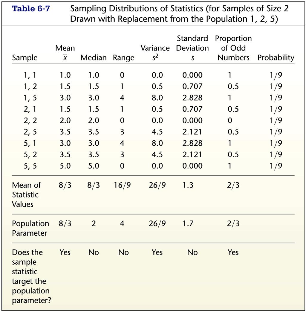
57 Slide 57

58 Sampling Distributions A population consists of the values 1, 2, and 5. We randomly select samples of size 2 with replacement. There are 9 possible samples. b. For each statistic, find the mean from part (a) The means are found near the bottom of Table 6-7. Slide 58

59 Interpretation of Sampling Distributions We can see that when using a sample statistic to estimate a population parameter, some statistics are good in the sense that they target the population parameter and are therefore likely to yield good results. Such statistics are called unbiased estimators. Statistics that target population parameters: mean, variance, proportion Statistics that do not target population parameters: median, range, standard deviation Slide 59

60 Recap In this section we have discussed: Sampling distribution of a statistic. Sampling distribution of a proportion. Sampling distribution of the mean. Sampling variability. Estimators. Slide 60

61 Section 6-5 The Central Limit Theorem Created by Erin Hodgess, Houston, Texas Revised to accompany 10 th Edition, Tom Wegleitner, Centreville, VA Slide 61

62 Key Concept The procedures of this section form the foundation for estimating population parameters and hypothesis testing topics discussed at length in the following chapters. Slide 62

63 Central Limit Theorem Given: 1. The random variable x has a distribution (which may or may not be normal) with mean µ and standard deviation σ. 2. Simple random samples all of size n are selected from the population. (The samples are selected so that all possible samples of the same size n have the same chance of being selected.) Slide 63

64 Central Limit Theorem - cont Conclusions: 1. The distribution of sample x will, as the sample size increases, approach a normal distribution. 2. The mean of the sample means is the population mean µ. 3. The standard deviation of all sample means is σ/. n Slide 64

65 Practical Rules Commonly Used 1. For samples of size n larger than 30, the distribution of the sample means can be approximated reasonably well by a normal distribution. The approximation gets better as the sample size n becomes larger. 2. If the original population is itself normally distributed, then the sample means will be normally distributed for any sample size n (not just the values of n larger than 30). Slide 65

66 Notation the mean of the sample means µ x = µ the standard deviation of sample mean σ x = σ n (often called the standard error of the mean) Slide 66

67 Simulation With Random Digits Generate 500,000 random digits, group into 5000 samples of 100 each. Find the mean of each sample. Even though the original 500,000 digits have a uniform distribution, the distribution of 5000 sample means is approximately a normal distribution! Slide 67

68 Important Point As the sample size increases, the sampling distribution of sample means approaches a normal distribution. Slide 68

69 Example Water Taxi Safety Given the population of men has normally distributed weights with a mean of 172 lb and a standard deviation of 29 lb, a) if one man is randomly selected, find the probability that his weight is greater than 175 lb. b) if 20 different men are randomly selected, find the probability that their mean weight is greater than 175 lb (so that their total weight exceeds the safe capacity of 3500 pounds). Slide 69

70 Example cont a) if one man is randomly selected, find the probability that his weight is greater than 175 lb. z = = Slide 70

71 Example cont b) if 20 different men are randomly selected, find the probability that their mean weight is greater than 172 lb. z = = Slide 71

72 Example - cont a) if one man is randomly selected, find the probability that his weight is greater than 175 lb. P(x > 175) = b) if 20 different men are randomly selected, their mean weight is greater than 175 lb. P(x > 175) = It is much easier for an individual to deviate from the mean than it is for a group of 20 to deviate from the mean. Slide 72

73 Interpretation of Results Given that the safe capacity of the water taxi is 3500 pounds, there is a fairly good chance (with probability ) that it will be overloaded with 20 randomly selected men. Slide 73

74 Correction for a Finite Population When sampling without replacement and the sample size n is greater than 5% of the finite population of size N, adjust the standard deviation of sample means by the following correction factor: N n σ x = σ n N 1 finite population correction factor Slide 74

75 Recap In this section we have discussed: Central limit theorem. Practical rules. Effects of sample sizes. Correction for a finite population. Slide 75

76 Section 6-6 Normal as Approximation to Binomial Created by Erin Hodgess, Houston, Texas Revised to accompany 10 th Edition, Tom Wegleitner, Centreville, VA Slide 76

77 Key Concept This section presents a method for using a normal distribution as an approximation to the binomial probability distribution. If the conditions of np 5 and nq 5 are both satisfied, then probabilities from a binomial probability distribution can be approximated well by using a normal distribution with mean μ = np and standard deviation σ = npq Slide 77

78 Review Binomial Probability Distribution 1. The procedure must have fixed number of trials. 2. The trials must be independent. 3. Each trial must have all outcomes classified into two categories. 4. The probability of success remains the same in all trials. Solve by binomial probability formula, Table A-1, or technology. Slide 78

79 Approximation of a Binomial Distribution with a Normal Distribution np 5 nq 5 then µ = np and σ = npq and the random variable has a (normal) distribution. Slide 79

80 Procedure for Using a Normal Distribution to Approximate a Binomial Distribution 1. Establish that the normal distribution is a suitable approximation to the binomial distribution by verifying np 5 and nq Find the values of the parameters µ and σ by calculating µ = np and σ = npq. 3. Identify the discrete value of x (the number of successes). Change the discrete value x by replacing it with the interval from x 0.5 to x (See continuity corrections discussion later in this section.) Draw a normal curve and enter the values of µ, σ, and either x 0.5 or x + 0.5, as appropriate. Slide 80

81 Procedure for Using a Normal Distribution to Approximate a Binomial Distribution - cont 4. Change x by replacing it with x 0.5 or x + 0.5, as appropriate. 5. Using x 0.5 or x (as appropriate) in place of x, find the area corresponding to the desired probability by first finding the z score and finding the area to the left of the adjusted value of x. Slide 81

82 Example Number of Men Among Passengers Finding the Probability of At Least 122 Men Among 213 Passengers Figure 6-21 Slide 82

83 Definition When we use the normal distribution (which is a continuous probability distribution) as an approximation to the binomial distribution (which is discrete), a continuity correction is made to a discrete whole number x in the binomial distribution by representing the single value x by the interval from x 0.5 to x (that is, adding and subtracting 0.5). Slide 83

84 Procedure for Continuity Corrections 1. When using the normal distribution as an approximation to the binomial distribution, always use the continuity correction. 2. In using the continuity correction, first identify the discrete whole number x that is relevant to the binomial probability problem. 3. Draw a normal distribution centered about µ, then draw a vertical strip area centered over x. Mark the left side of the strip with the number x 0.5, and mark the right side with x For x = 122, draw a strip from to Consider the area of the strip to represent the probability of discrete whole number x. Slide 84

85 Procedure for Continuity Corrections - cont 4. Now determine whether the value of x itself should be included in the probability you want. Next, determine whether you want the probability of at least x, at most x, more than x, fewer than x, or exactly x. Shade the area to the right or left of the strip, as appropriate; also shade the interior of the strip itself if and only if x itself is to be included. The total shaded region corresponds to the probability being sought. Slide 85

86 Figure 6-22 x = at least 122 (includes 122 and above) x = more than 122 (doesn t include 122) x = at most 122 (includes 122 and below) x = fewer than 122 (doesn t include 122) x = exactly 122 Slide 86

87 Recap In this section we have discussed: Approximating a binomial distribution with a normal distribution. Procedures for using a normal distribution to approximate a binomial distribution. Continuity corrections. Slide 87

88 Section 6-7 Assessing Normality Created by Erin Hodgess, Houston, Texas Revised to accompany 10 th Edition, Tom Wegleitner, Centreville, VA Slide 88

89 Key Concept This section provides criteria for determining whether the requirement of a normal distribution is satisfied. The criteria involve visual inspection of a histogram to see if it is roughly bell shaped, identifying any outliers, and constructing a new graph called a normal quantile plot. Slide 89

90 Definition A normal quantile plot (or normal probability plot) is a graph of points (x,y), where each x value is from the original set of sample data, and each y value is the corresponding z score that is a quantile value expected from the standard normal distribution. Slide 90

91 Methods for Determining Whether Data Have a Normal Distribution 1. Histogram: Construct a histogram. Reject normality if the histogram departs dramatically from a bell shape. 2. Outliers: Identify outliers. Reject normality if there is more than one outlier present. 3. Normal Quantile Plot: If the histogram is basically symmetric and there is at most one outlier, construct a normal quantile plot as follows: Slide 91

92 Procedure for Determining Whether Data Have a Normal Distribution - cont 3. Normal Quantile Plot a. Sort the data by arranging the values from lowest to highest. b. With a sample size n, each value represents a proportion of 1/n of the sample. Using the known sample size n, identify the areas of 1/2n, 3/2n, 5/2n, 7/2n, and so on. These are the cumulative areas to the left of the corresponding sample values. c. Use the standard normal distribution (Table A-2, software or calculator) to find the z scores corresponding to the cumulative left areas found in Step (b). Slide 92

93 Procedure for Determining Whether Data Have a Normal Distribution - cont d. Match the original sorted data values with their corresponding z scores found in Step (c), then plot the points (x, y), where each x is an original sample value and y is the corresponding z score. e. Examine the normal quantile plot using these criteria: If the points do not lie close to a straight line, or if the points exhibit some systematic pattern that is not a straight-line pattern, then the data appear to come from a population that does not have a normal distribution. If the pattern of the points is reasonably close to a straight line, then the data appear to come from a population that has a normal distribution. Slide 93

94 Example Interpretation: Because the points lie reasonably close to a straight line and there does not appear to be a systematic pattern that is not a straight-line pattern, we conclude that the sample appears to be a normally distributed population. Slide 94

95 Recap In this section we have discussed: Normal quantile plot. Procedure to determine if data have a normal distribution. Slide 95