NCHRP Consequences of Delayed Maintenance

Transcription

1 NCHRP Consequences of Delayed Maintenance Recommended Process for Bridges and Pavements prepared for NCHRP prepared by Cambridge Systematics, Inc. with Applied Research Associates, Inc. Spy Pond Partners January

2

3 report NCHRP Consequences of Delayed Maintenance Recommended Process for Bridges and Pavements prepared for NCHRP prepared by Cambridge Systematics, Inc. 115 South LaSalle Street, Suite 2200 Chicago, IL with Applied Research Associates, Inc. Spy Pond Partners date January 2012

4

5 Table of Contents 1.0 Introduction Quantifying the Consequences of Delayed Maintenance Conceptual Framework Defining the Relationship between Cost and Level of Service An Alternative Approach to Quantifying the Consequences of Delayed Maintenance Step-by-Step Process Step 1. Define Key Assumptions Step 1.1. Define Maintenance Step 1.2. Identify Metrics for the Analysis Step 1.3. Define a Delay Period Step 1.4. Define a Catch-Up Period Step 1.5. Define a Discount Rate Step 2. Define a Network of Assets Step 3. Develop Activity Costs Step 4. Develop Asset Deterioration Models Step 5. Develop a Preferred Maintenance Policy Step 6. Define a Delayed Maintenance Policy Step 7. Estimate Costs and Conditions for the Baseline Scenario Step 8. Estimate Costs and Conditions for the Delayed Maintenance Scenario Step 9. Quantify the Consequences of Delayed Maintenance Bridge Example Step 1. Define Key Assumptions Step 1.1. Define Maintenance Step 1.2. Identify a Level of Service Metric Step 1.3. Define a Delay Period Step 1.4. Define a Catch-Up Period Step 1.5. Define a Discount Rate Step 2. Define a Network of Assets Step 3. Develop Activity Costs Step 4. Develop Asset Deterioration Models Cambridge Systematics, Inc i

6 Table of Contents, continued Step 5. Develop a Preferred Maintenance Policy Step 6. Define a Delayed Maintenance Policy Step 7. Estimate Costs and Conditions for the Baseline Scenario Step 8. Estimate Costs and Conditions for the Delayed Maintenance Scenario Step 9. Quantify the Consequences of Delayed Maintenance Pavement Example Step 1. Define Key Assumptions Step 1.1. Define Maintenance Step 1.2. Identify a Level of Service Metric Step 1.3. Define a Delay Period Step 1.4. Define a Catch-Up Period Step 1.5. Define a Discount Rate Step 2. Develop Activity Costs Step 3. Define a Network of Assets Step 4. Develop Asset Deterioration Models Data Pertaining to Pavement Performance Modeling Developing a Performance Database and Models Step 5. Develop a Preferred Maintenance Policy Step 6. Define a Delayed Maintenance Policy Step 7. Estimate Costs and Conditions for the Baseline Scenario Step 8. Estimate Costs and Conditions for the Delayed Maintenance Scenario Step 9. Quantify the Consequences of Delayed Maintenance ii Cambridge Systematics, Inc

7 List of Tables Table 4.1 Excerpt of Maintenance Activities by Condition State and Action for Bare Concrete Deck Table 4.2 Illustrative Example of Concrete Deck Element Conditions Table 4.3 Table 4.4 Table 4.5 Table 4.6 Example Activity Costs Bare Concrete Deck, Wet Freeze Environment Example Deterioration Model Bare Concrete Deck, Wet Freeze Environment Example Preferred Maintenance Policy Bare Concrete Deck, Wet Freeze Environment Example Delayed Maintenance Policy Bare Concrete Deck, Wet Freeze Environment Table 5.1 Kansas DOT Maintenance Cost Table Table 5.2 Performance Models Developed for the Pilot Table 5.3 Summary of the Transverse Cracking Models Coefficients Table 5.4 Summary of the Rutting Model Coefficients Table 5.5 Summary of the IRI Model Coefficients Table 5.6 Kansas DOT Maintenance Treatment Matrix Cambridge Systematics, Inc. iii

8

9 List of Figures Figure 2.1 Conceptual Modeling Framework, Scenario Figure 2.2 Conceptual Modeling Framework, Scenario Figure 2.3 Example Relationship between Bridge Level of Service and Budget Figure 2.4 Example Relationship between Pavement Level of Service and Budget Figure 2.5 Quantifying the Cost of Achieving Improved Conditions Figure 2.6 Baseline Scenario Figure 2.7 Delayed Maintenance Scenario Figure 4.1 Agency Costs for the Baseline Scenario Figure 4.2 User Costs for the Baseline Scenario Figure 4.3 Health Index for the Baseline Scenario Figure 4.4 Agency Costs for the Delayed Maintenance Scenario Figure 4.5 User Costs for the Delayed Maintenance Scenario Figure 4.6 Network Health Index for the Delayed Maintenance Scenario Figure 4.7 Agency Cost Comparison Figure 4.8 User Cost Comparison Figure 4.9 Health Index Comparison Figure 5.1 Interstate 70 and US 400 Highway Corridors across Kansas Figure 5.2 Example Plot of IRI versus Age for One Segment Figure 5.3 Predicted Transverse Cracking for Different Pavement Types Figure 5.4 Predicted Rutting for Different Pavement Types Figure 5.5 Predicted IRI for Different Pavement Types Figure 5.6 Regression Statistics of the Global Performance Models Figure 5.7 NPV of Agency Costs for the Baseline Scenario Figure 5.8 NPV of Agency Costs for the Delayed Maintenance Scenario Figure 5.9 Comparison of Agency Costs (NPV) Cambridge Systematics, Inc. v

10

11 1.0 Introduction Highway agencies apply various maintenance treatments to slow asset deterioration and restore pavements, bridges, and other assets to an acceptable condition. However, budget constraints and other factors can lead agencies to consider delaying or eliminating these treatments. The goal of National Cooperative Highway Research Program (NCHRP) project is to define a process for quantifying the consequences of delayed maintenance. This document discusses the relationship between asset condition and funding level, defines a process for quantifying the consequences of delaying bridge and pavement maintenance, and provides examples of its application. The recommended process consists of the following steps: 1. Define key assumptions. 1.1 Define maintenance. 1.2 Identify a level of service metric. 1.3 Define a delay period. 1.4 Define a catch-up period. 1.5 Define a discount rate. 2. Define a network of assets. 3. Estimate activity costs. 4. Develop asset deterioration models. 5. Develop a preferred maintenance policy (this policy will be followed during the baseline scenario). 6. Develop a delayed maintenance policy (this policy will be followed during the delayed maintenance scenario). 7. Estimate the costs and condition for the baseline scenario. 8. Estimate the costs and condition of the delayed maintenance scenario. 9. Estimate the consequences of delayed maintenance. Key characteristics of this process include the following: The process is flexible and provides custom results. The consequences of delaying maintenance vary greatly depending on a number of key variables such as the size and condition of the network being analyzed, the activities delayed, the length of the delay, etc. The process described in this document enables agencies to select variables that reflect their current situation and generate custom results. Cambridge Systematics, Inc. 1-1

12 The process is practical. This document illustrates two examples of the application of the process: one for bridges and one for pavements. The bridge example relies on national default bridge models and an existing data set that every department of transportation (DOT) can access. The pavement example illustrates the use of a DOT s customized pavement data and pavement management policies. An agency can elect to apply either of these approaches to quantify the consequences of delayed maintenance. The process addresses changes in agency costs, levels of service, and user costs. As an asset deteriorates due to delayed maintenance, it eventually will reach a point when more expensive work is required (e.g. asset replacement). Over time, the level of service provided to the traveling public will decrease and the user costs associated with using the asset will increase. (In this context and throughout this report, the term condition is used synonymously with the term level of service. ) The recommended approach addresses these three types of consequences. The process takes advantage of best practices in bridge and pavement modeling. State of the art bridge and pavement management systems enable agencies to predict how an asset will deteriorate over time, and can be used to assess the relationship between funding level and resulting levels of service. The recommended process takes advantage of these capabilities to create a lightweight, sketch-level tool for quantifying the consequences of delayed maintenance. The remainder of this document is organized as follows: Section 2 provides a conceptual framework for determining the consequences of delayed bridge and pavement maintenance; discusses how agencies can determine the relationship between funding level and level of service; and provides an overview of the recommended process. Section 3 provides a detailed, step-by-step process for quantifying the consequences of delayed maintenance and describes inputs, outputs, limitations, assumptions, and other relevant information required for implementation. Section 4 presents an example application of the recommended process for bridges. Section 5 presents an example application of the process for pavements. 1-2 Cambridge Systematics, Inc.

13 2.0 Quantifying the Consequences of Delayed Maintenance 2.1 CONCEPTUAL FRAMEWORK Figures 2.1 and Figure 2.2 illustrate a conceptual framework for assessing the relationship between asset level of service, required maintenance work, and costs. Cambridge Systematics, Inc. 2-1

14 Figure 2.1 illustrates a scenario in which maintenance is performed. It reflects the following cycle: An asset has a specified starting condition (illustrated by point A in the figure). Over time, the asset deteriorates and the condition decreases. Eventually it reaches a predefined condition threshold at which work is recommended (point B). The recommended work is performed, a cost is incurred, and the condition improves (point C). The asset again begins to deteriorate until additional work is recommended (point D). Again, the recommended work is performed, a cost is incurred, and the condition improves (point E). This cycle is repeated over the life of the asset. Figure 2.1 Conceptual Modeling Framework, Scenario 1 A C E B D 2-2 Cambridge Systematics, Inc.

15 Figure 2.2 shows an alternative scenario in which maintenance is delayed. This scenario reflects the following cycle: An asset has the same starting condition as the previous scenario (point A). It again reaches a predefined condition threshold at which work is recommended (point B). In this scenario however, the recommended work is not performed, and the asset continues to decrease until a point at which more expensive work is recommended (point C). The more expensive work is performed, a higher cost is incurred by the agency (higher relative to the cost incurred if work had been performed at point B), and the condition improves (point D). Figure 2.2 Conceptual Modeling Framework, Scenario 2 A D B C The relationships between asset condition, recommended work, and agencies cost illustrated in Figures 2.1 and 2.2 are critical for estimated the consequences of delayed bridge and pavement maintenance. 2.2 DEFINING THE RELATIONSHIP BETWEEN COST AND LEVEL OF SERVICE State-of-the-art bridge and pavement management systems enable agencies to use the process illustrated in Figures 2.1 and 2.2 to explicitly define the relationship between costs and level of service. Once the relationship between Cambridge Systematics, Inc. 2-3

16 costs and level of service is determined, agencies can answer two types of fundamental questions: What would be the cost of achieving a higher or lower level of service? What level of service could be achieved for a higher or lower budget? An example is shown in Figure 2.3. This figure shows the expected level of service (expressed as percent of deck area in good condition) in 2035 for various funding levels for bridges in the Indianapolis, Indiana region. For example, the figure indicates that achieving 50 percent of deck in good condition would cost about $180 million annually (point A), and achieving 60 percent in good condition would cost about $270 million annually (point B). Figure 2.3 Example Relationship between Bridge Level of Service and Budget Percent of Bridge Deck area in Good Condition (2035) 100% 80% 60% 40% A 20% 0% Annual Budget (millions) 2-4 Cambridge Systematics, Inc.

17 This graph was created using standard output from a Federal Highway Administration (FHWA) tool called National Bridge Investment Analysis System (NBIAS), which uses a modeling approach consistent with that illustrated in Figure The modeling approach can be summarized as follows: In year 1 of the analysis, work activities are flagged by comparing the condition of each asset to a previously defined set of condition thresholds. Each activity is assigned a cost. Users specify a budget. The system prioritizes the potential activities, and selects them until the budget is expended. The system then projects conditions into the next year. If work was done on an asset, its condition improves. If not, its condition deteriorates. The selection of activities and modeling of results is repeated for each year of the analysis. The system provides the projected level of service (along with other metrics) at the end of the analysis period. 1 For detailed information on the NBIAS modeling approach and how to use the system, refer to its technical manual and user manual. Cambridge Systematic, National Bridge Investment Analysis (NBIAS) Version 3.4 Technical Manual, developed for the Federal Highway Administration, April Cambridge Systematic, National Bridge Investment Analysis (NBIAS) Version 3.4 User Manual, developed for the Federal Highway Administration, April Cambridge Systematics, Inc. 2-5

18 Similar figures can be developed using outputs from pavement management systems. For example, Figure 2.4 shows the relationship between pavement condition (in this case reported as the percent of pavement in good condition) and annual budget for the Indianapolis region. This graph was created using standard output from a FHWA tool called the Highway Economic Requirements System State Version (HERS-ST). 2 Prior to the analysis, HERS-ST was configured so that only maintenance activities would be considered. Figure 2.4 Example Relationship between Pavement Level of Service and Budget Percent of Pavement in Good Condition (2035) 100% 80% 60% 40% 20% 0% Annual Budget (millions) It is important to note that there is no single relationship between cost and asset level of service. The framework illustrated in Figure 2.1 is dependent on the size of the inventory being analyzed, the distribution of the network s current conditions, and the expected deterioration rates for the assets in the network (which are dependent on factors such as weather and traffic volumes). Therefore the relationships between costs and level of service illustrated in Figure 2.3 and 2.4 are specific for the highway and bridge network in the Indianapolis region. Different networks, comprising different quantities of different types of assets in different starting conditions with different levels of traffic would yield very different results. 2 For detailed information on the HERS-ST modeling approach and how to use the system, refer to its user s guide. FHWA, HERS-ST User s Guide, Cambridge Systematics, Inc.

19 It is also important to note that even though these examples were developed with FHWA tools, agencies can develop similar curves with whatever bridge and pavement management system they use. And, therefore, the process for developing these curves will vary based on the tool being used. For example, NBIAS generates this type of curve almost automatically, as it is designed to simultaneously evaluate multiple funding levels. In contrast, developing the pavement relationship in Figure 2.4 required updating HERS-ST parameters to ensure that only preservation-related activates were considered, and then running several funding scenarios manually and combining the resulting condition values for each scenario. Regardless of the tool being used, generating these types of figures requires the following general steps: Ensure that the tool will model only actions considered to be maintenance. Define a network of assets and a time horizon (the examples above reflect a 25-year time frame). Select a level of service metric. Select a funding level and use the tool to predict the level of service that could be achieved given that funding level. Repeat the process for several funding levels. Plot the results. Once developed, the types of curves illustrated in Figures 2.3 and 2.4 enable agencies to understand and communicate the relationship between budget and level of service. By comparing the graph to existing conditions, agencies also could use them to quantify the costs associated with achieving an improved level of service. Cambridge Systematics, Inc. 2-7

20 For example, Figure 2.5 repeats Figure 2.4, but shows two additional points on the graph. Consider a case in which point A represents the current level of service (70 percent pavement in good condition in 2035). The graph shows that maintaining this condition through 2035 would cost about $188 million annually. If an agency wanted to improve the level of service to 90 percent condition level (point B), it would cost about $235 million annually; an increase of $47 million per year. Figure 2.5 Quantifying the Cost of Achieving Improved Conditions Percent of Pavement in Good Condition (2035) 100% B 80% 60% A 40% 20% 0% Annual Budget (millions) These types of curves also enable agencies to quantify the consequences of delayed maintenance. For example, if point B in Figure 2.5 indicates current funding levels ($235 million per year), any reduction in funding would predicate a reduction in level of service. Therefore, it is possible to estimate the consequences of delayed maintenance by finding a lower budget level on the graph and the resulting level of service. For example, if the current budget allocates $235 million per year to pavement maintenance (point B) and the budget is reduced to $188 million per year (point A), then the level of service is expected to decrease from 90 percent (point B) to 70 percent (point A). A change in level of service is one of the consequences of delaying maintenance. Another potential consequence is a change in user costs (i.e., the costs that the traveling public incur while using an asset). NBIAS and HERS-ST both include models that relate asset condition to vehicle operating costs (as conditions get worse, drive time and vehicle wear and tear increase). Therefore, these tools (and potentially other agency-specific management systems) could be used to 2-8 Cambridge Systematics, Inc.

21 develop graphs similar to Figure 2.3 and 2.4 except with user costs on the y-axis rather than measures of level of service. 2.3 AN ALTERNATIVE APPROACH TO QUANTIFYING THE CONSEQUENCES OF DELAYED MAINTENANCE The examples in section 2.2 illustrate one approach to quantifying the consequences of delayed maintenance: exercise management systems in order to determine the relationship between level of service (and/or user costs) and maintenance budget. The NCHRP research team has taken the basic modeling approach inherent in asset management systems, and used it to develop a new, more flexible and comprehensive process. In addition to addressing changes in level of service and user costs due to delayed maintenance, the new process also estimates the impact on agency costs. In the approach described above, agency costs are handled as an input. A user specifies a budget level, and a management system is used to determine which work should be done with these funds, and the impact of this work on level of service. In the new process, agency costs are handled as an output. This process is best explained by revisiting Figures 2.1 and 2.2, which were introduced at the beginning of this section. Cambridge Systematics, Inc. 2-9

22 Figure 2.6 now reflects a baseline scenario. In this scenario, a preferred maintenance policy is defined and followed. In this context, the term preferred maintenance policy refers to a set of condition thresholds at which work should be performed. Figure 2.6 Baseline Scenario 2-10 Cambridge Systematics, Inc.

23 Figure 2.7 now reflects a delayed maintenance scenario. In this scenario, work recommended by the preferred maintenance policy is delayed until after the delay period ends. Figure 2.7 Delayed Maintenance Scenario Delay period As the delay period lengthens, the cost incurred at the end of it eventually will exceed the cumulative costs incurred in the baseline scenario. The difference in the net present value (NPV) of these two cost streams represents the change in agency costs due to delayed maintenance. In the new approach, changes in agency costs are considered along with changes in network condition and changes in user costs. For example, at the end of the delay period, the difference in network conditions between baseline scenario and the delayed maintenance scenario reflects another consequence of delayed maintenance. Section 3 presents a step-by-step process for following the approach described above. Sections 4 and 5 provide example applications of the recommended approach. Cambridge Systematics, Inc. 2-11

24

25 3.0 Step-by-Step Process This section describes a step-by-step process for quantifying the consequences of delayed bridge and pavement maintenance. It also provides brief summaries of the approach used for each step for the bridge and pavement examples. For more details on these example applications refer to sections 4 and 5. These examples are provided to illustrate the application of the recommended process. The process is flexible so that agencies can change any of the assumptions and data items used in the examples. Agencies are strongly encouraged to take advantage of this flexibility, and set up the analysis in a manner that best reflects their operating environment. The recommended process consists of the following steps: 1. Define key assumptions. 1.1 Define maintenance. 1.2 Identify a level of service metric. 1.3 Define a delay period. 1.4 Define a catch-up period. 1.5 Define a discount rate. 2. Define a network of assets. 3. Estimate activity costs. 4. Develop asset deterioration models. 5. Develop a preferred maintenance policy (this policy will be followed during the baseline scenario). 6. Develop a delayed maintenance policy (this policy will be followed during the delayed maintenance scenario). 7. Estimate the costs and condition for the baseline scenario. 8. Estimate the costs and condition of the delayed maintenance scenario. 9. Calculate the consequences of delayed maintenance. STEP 1. DEFINE KEY ASSUMPTIONS Step 1.1. Define Maintenance Although the American Association of State Highway and Transportation Officials (AASHTO) and FHWA have worked to develop standard maintenance definitions, most agencies have developed custom definitions of maintenance to Cambridge Systematics, Inc. 3-1

26 meet their specific needs. Therefore, the recommended approach is flexible and allows agencies to define maintenance in a manner that matches their internal definitions. Implementation activities: Define maintenance by developing a list of specific work activities that will be included in the analysis. Bridge example: Maintenance was defined as the set of maintenance, rehabilitation, and replacement actions used by NBIAS. Pavement example: Maintenance was defined by asking staff from the Kansas Department of Transportation (DOT) to identify appropriate pavement maintenance activities. (The process of defining key variables based on the expertise and judgment of agency staff is referred to as expert elicitation. ) Step 1.2. Identify Metrics for the Analysis At its core, the recommended process is driven by the relationship between level of service, recommended maintenance activities, and costs. At least one measure of physical asset condition is needed that meets the following criteria: Current values of the metric can be provided for each asset in the selected network; Deterioration rates reflecting how the metric is expected to change over time can be developed; Thresholds for the metric can be defined that indicate when maintenance work is recommended; and Models can be developed that reflect the impact of maintenance activities on the value of the metric. In addition to measures of asset condition, the process can account for user costs. If user costs will be considered, a model relating user costs to asset condition will need to be developed as part of step 4. Implementation activities: Define at least one measure of physical condition to be used throughout the analysis. Determine if user costs will be included in the analysis. Bridge example: Bridge Health Index. User costs were considered in the analysis. Pavement example: Transverse cracking (cracks/mile), rutting (inches), and International Roughness Index (IRI) (inches/mile). User costs were not considered. Step 1.3. Define a Delay Period The recommended process is flexible in terms of the delay period that can be analyzed. In order to select an appropriate period, agencies must assess the 3-2 Cambridge Systematics, Inc.

27 purpose for quantifying the consequences of delayed maintenance and the intended audience for the results. For example, an agency may need to support discussion regarding mid-term funding (e.g., 5-10 years). Alternatively, an agency may need to support long range planning discussions, which may require a longer-term (20 to 30 years) analysis of the impacts of different funding levels, as illustrated in section 2. How the assumption impacts results: Given the steep deterioration at the tailend of classic asset deterioration curves, as illustrated in Figure 2.1, longer delay periods will increase the cost of delayed maintenance. Note that the discount rate (step 1.5) and the starting condition of the network (step 2) will significantly influence the impact of the analysis period. For example, there likely will be no cost consequences of delaying maintenance for a couple of years on a bridge network that is currently in excellent condition. However, the consequences will appear if maintenance is delayed long enough. Implementation activities: Define a delay period. Bridge example: 10 years. Pavement example: 5 years. The research team focused the bridge and pavement examples on scenarios in which maintenance is delayed temporarily rather than dimensioned over a long period. Step 1.4. Define a Catch-Up Period The process assumes that after the delay period has ended, there will be a catchup period during which an agency addresses the accumulated backlog of work. (The cost of addressing this backlog reflects the lost of economic value associated with a network deteriorating.) Including the costs accrued during the catch-up period and the impact of this work on system condition will help agencies to assess the full consequences of delayed maintenance. How the assumption impacts results: A catch-up period that is too short (for example, one to two years) may not fully capture the costs of delayed maintenance because some of the inherent backlog (and loss of overall asset valuation) would need to be addressed after the analysis period. For example, the full cost implications of multiple, ill-timed thin overlays may not surface in a single year. Implementation activities: Define a catch-up period (the recommended value is five or more years). Bridge example: Five years. Pavement example: 10 years. Step 1.5. Define a Discount Rate The recommended process involves capturing agency costs incurred each year throughout the delay period and the catch-up period. In order to directly Cambridge Systematics, Inc. 3-3

28 compare results across multiple scenarios, these costs are then converted to a Net Present Value (NPV). Calculating an NPV requires a discount rate. In the NPV calculation, all future costs are discounted to today s dollars and summed. In circular A-94, the Office of Management and Budget (OMB) provides guidance on two types of discount rates: one used for federal benefit/cost analysis and one used for cost-effectiveness analysis. 3 The discount rate recommended for benefit/cost analysis is based on the return rate in the private market and is meant to reflect the time-cost of money. In their national asset management systems, FHWA has elected to a discount rate of seven percent. The discount rate recommended by OMB circular A-94 for cost-effectiveness analysis is based on the U.S. Treasury borrowing rate on marketable securities of comparable maturity to the period of analysis. Agencies may elect to apply the cost-effectiveness analysis discount rate using OMB circular A-94 tables describing the discount rate by length of the project (e.g. for a 10 year analysis period, the discount rate currently is 1.3 percent). How the assumption impacts results: The discount rates will impact the consequences of delayed maintenance. Higher discount rates will discount future agency and user costs, lessening their NPV. If a life cycle cost analysis is used (refer to step 4), higher rates will tend to push maintenance actions to be less aggressive in the near-term and more aggressive in the long-term based on a trade-off of current savings versus lower future costs. In addition, higher discount rates tend to discount the consequences of delayed maintenance because future costs will be lower relative to current costs. Conversely, a lower discount rate will result in a higher NPV of costs, making agencies more aggressive in the near-term and increasing the consequences of delayed maintenance. Implementation activities: Define a discount rate. While OMB circular A-94 provides guidance on establishing a discount rate, it is recommended that agencies use a discount rate that is consistent with their other economic analysis efforts. Bridge example: 1.3 percent, based on the 2011 rate recommended in OMB Circular A-94 for cost-effectiveness analysis for a 10-year analysis period. 4 After reviewing the OMB guidance, the study team felt that the assessment of the consequences of delayed maintenance reflected more of a cost-effectiveness analysis than a benefit-cost analysis. The basis for this decision is an assumption 3 U.S. Office of Management and Budget, Circular A-94 Revised, October (Appendix C, which recommends interest rates for cost effectiveness analysis, is updated annually.) 4 Between the time the analysis was conducted for the examples, and the writing of this document, OMB updated their recommendations. The recommended rate for 2012 is 1.1 percent. 3-4 Cambridge Systematics, Inc.

29 that any decrease in maintenance funds would be allocated to some of type of project or services within the agency, not returned to the private investment market. Pavement example: 1.3 percent for the same reasons described above for the bridge example. STEP 2. DEFINE A NETWORK OF ASSETS The process requires defining a specific network of assets. The network can include any collection of assets (e.g., all state owned assets, Interstate assets, assets along specific corridors, etc.). The selection of the network will have a significant impact on the consequences of delayed maintenance, because the approach is conducted asset-by-asset based on its current condition. Delaying maintenance on larger networks in worse condition will have higher consequences then delaying maintenance on smaller networks in better condition. Input: Inventory and condition information stored in an agency database. Implementation activities: Define a network of assets. Output: A network of assets, including its extent (e.g., lane miles) and current condition. Bridge example: An illustrative network of bridges. Pavement example: Interstate 70 and State Route 400 running through Kansas. STEP 3. DEVELOP ACTIVITY COSTS A cost estimate for each maintenance activity is required in order to track cost streams over time and, ultimately, quantify the consequences of delayed maintenance. Options for this step include using national default costs, using previously developed state unit costs, analyzing historic cost data stored in a state database, and conducting an expert elicitation. Input: List of maintenance activities (from Step 1.1) Implementation activities: For each activity, develop a unit cost. Output: A unit costs for each activity included in the analysis. Bridge example: Unit costs developed by FHWA for use in NBIAS. Pavement example: Unit costs based on a review of recently completed maintenance projects in Kansas. Cambridge Systematics, Inc. 3-5

30 STEP 4. DEVELOP ASSET DETERIORATION MODELS The process requires a set of asset models that define 1) how quickly an asset will deteriorate, and 2) how asset conditions will be impacted when the maintenance activities are performed. Options for this step include using national default models, using previously developed state models, analyzing historic inspection and project data, or conducting an expert elicitation. Input: Level of service metrics (from Step 1.2) and list of maintenance activities (from Step 1.1). Implementation activities: For each asset type (e.g., bridge element or pavement type), define a rate of annual deterioration and identify the impact of each maintenance action on the metric. If user costs are included in the analysis, develop an approach for estimating them based on asset condition. Output: Asset deterioration model, estimates regarding the response of condition to each maintenance activity, and an approach for calculating user costs. Bridge example: National default models developed by FHWA for use in NBIAS. The models vary by climate zone. The NBIAS user costs model is based on bridge deck condition. Pavement example: Custom pavement deterioration models based on data from the Kansas DOT. The models have been tailored for the two corridors included in the analysis. User costs were not address in this example, but could be derived from IRI values. STEP 5. DEVELOP A PREFERRED MAINTENANCE POLICY The recommended process requires a preferred maintenance policy that defines condition thresholds at which each maintenance activity should be performed. There are two common approaches for developing preferred maintenance policies: life cycle cost analysis (LCCA) and expert elicitation. LCCA is used to identify optimal maintenance policies that minimize long-term agency and/or user costs. Expert elicitation is used to identify maintenance actions based on agency experience and engineering judgment. Either method is suitable for use in defining the preferred maintenance policy. Input: Varies based on approach used. Any approach will require a list of maintenance activities (step 1.1) and a level of service metric (step 1.2). In addition, LCCA requires an optimization process that combines asset deterioration models (step 4), activity costs (step 3), and a discount rate (step 1.5) to identify a policy that will achieve the minimum long-term cost. Expert 3-6 Cambridge Systematics, Inc.

31 elicitation requires historical perspective and expertise gathered through a facilitated process. Implementation activities: For each asset type and each condition level, identify the preferred maintenance action. The actions should include do nothing. Output: A preferred maintenance policy identifying the preferred maintenance activity for each asset type for each condition level. Bridge example: Policy developed using NBIAS, which is based on LCCA of agency and user costs. (The policy used for the example is based on a discount rate of 1.3 percent. The national default policy provided in NBIAS is based on a discount rate of seven percent.) Pavement example: Policy based on expert elicitation. STEP 6. DEFINE A DELAYED MAINTENANCE POLICY The recommended process also requires defining a set of actions to apply under the delayed maintenance scenario. For example, a delayed maintenance policy might be to simply do nothing, or to do something only when an asset fails. Input: List of potential maintenance activities (step 1.1). Implementation activities: Define what work will be performed during the delay period. Output: A delayed maintenance policy. Bridge example: Do nothing unless a bridge element fails, then replace that element. Pavement example: Do nothing. STEP 7. ESTIMATE COSTS AND CONDITIONS FOR THE BASELINE SCENARIO The consequences of delayed maintenance are based on a comparison of costs and conditions between a baseline scenario and a delayed maintenance scenario. This step addresses the baseline scenario. The other scenario is addressed in Step 8. Input: Output from all previous steps, except step 6 (delayed maintenance policy). Implementation activities: Apply the preferred maintenance policy to the selected network of assets, track network condition, track expenditures, track user costs (if included in the analysis), and calculate the NPV of all costs over the analysis and catch-up period. Cambridge Systematics, Inc. 3-7

32 Output: NPV of agency costs, NPV of user costs (if included in the analysis), and resulting condition level for the baseline scenario. Bridge example: Analysis was conducted using a prototype tool developed by the research team. Pavement example: Analysis was conducted using a prototype tool developed by the research team. STEP 8. ESTIMATE COSTS AND CONDITIONS FOR THE DELAYED MAINTENANCE SCENARIO The consequences of delayed maintenance are based on a comparison of costs and conditions between a baseline scenario and a delayed maintenance scenario. This step addresses the delayed maintenance scenario. The baseline scenario is addressed in step 7. Input: policy). Output from all previous steps, except step 5 (preferred maintenance Implementation activities: Apply the delayed maintenance policy to the selected network of assets, track network condition, track expenditures, track user costs (if included in the analysis), and calculate the NPV of all costs over the analysis and catch-up period. Output: NPV of agency costs, NPV of user costs (if included in the analysis), and resulting condition level for the baseline scenario. Bridge example: Analysis was conducted using a prototype tool developed by the research team. Pavement example: Analysis was conducted using a prototype tool developed by the research team. STEP 9. QUANTIFY THE CONSEQUENCES OF DELAYED MAINTENANCE This step combines the results from Steps 8 and 9 to quantify the consequences of delayed maintenance. Input: NPV of agency costs and user costs (if included in the analysis) and condition levels from the baseline scenario (step 7) and delayed maintenance scenario (step 8). Implementation activities: Subtract the NPV costs and condition levels of the baseline maintenance scenario from the NPV costs and condition levels of the delayed maintenance scenario. 3-8 Cambridge Systematics, Inc.

33 Output: The consequences of delayed maintenance as measured by the difference in condition, agency costs, and/or user costs between the base case and delayed maintenance scenarios. Cambridge Systematics, Inc. 3-9

34

35 4.0 Bridge Example This section walks through the step-by-step process for quantifying the costs of delayed bridge maintenance by way of example. The example illustrates one potential way the process can be implemented for bridges. The analysis was conducted using a prototype spreadsheet tool developed for this research effort that enables users to quickly perform sketch planning level analysis of the consequences of delayed bridge maintenance. Where appropriate, the narrative refers to elements of the spreadsheet, which can serve as a companion to the following descriptions. The prototype tool relies heavily on national default models developed by FHWA for use in NBIAS. For more information on the NBIAS modeling approach, refer to the NBIAS Technical Manual. 5 If an agency desires a more customized bridge analysis, it could either update the spreadsheet to reflect state-specific models and follow this example, or apply the more generic approach illustrated for pavements in section 5. STEP 1. DEFINE KEY ASSUMPTIONS Step 1.1. Define Maintenance In this example, bridge maintenance was defined as the set of maintenance, rehabilitation, and replacement (MR&R) actions used in NBIAS. In NBIAS, there are 72 elements; each element can have up to five condition states; and each condition state can have up to three different feasible actions. All told, there are 904 different maintenance actions. Table 4.1 provides an excerpt of the condition states and feasible maintenance activities for a bare concrete deck, and the full list of maintenance activities by element and condition. The prototype spreadsheet contains all of the maintenance actions. They are located in the mrractdefs tab where elemkey is the element number (refer to Elemdef for the long name); skey identifies the condition state; and akey identifies one appropriate maintenance activity for that condition. 5 Cambridge Systematic, National Bridge Investment Analysis (NBIAS) Version 3.4 Technical Manual, developed for the Federal Highway Administration, April Cambridge Systematics, Inc. 4-1

36 Table 4.1 Excerpt of Maintenance Activities by Condition State and Action for Bare Concrete Deck Condition State Feasible Activity 1 Do nothing 1 Add a protective system 2 Do nothing 2 Repair spalls and delaminations 2 Add a protective system 3 Do nothing 3 Repair spalls and delaminations 3 Repair spalls and delaminations,and add a protective system on entire deck 4 Do nothing 4 Repair spalls and delaminations 4 Repair spalls and delaminations and add a protective system on entire deck 5 Do nothing Repair spalls and delaminations and/or add a protective system on entire 5 deck 5 Replace deck Source: NBIAS, version 3.4 Step 1.2. Identify a Level of Service Metric The bridge Health Index provides a brief, comprehensive, simple to understand measure of the health of the bridge network, and can help decision makers to quickly assess the relative impacts of funding decisions. Health Index is reported on a continuous scale from 0 to 100, with 100 being the highest rating. Health Index represents a weighted average of element condition data. To aggregate element-level conditions, weights are assigned to the elements according to the economic consequences of element failure. Thus, elements whose failure would have relatively little economic effect receive less weight than elements whose failure could close a bridge. 6 The weights are defined in the Elemdef tab of the spreadsheet, and the network Health Index is calculated in the Input.Output tab. The bridge example also incorporates user costs, which are described further in Step 4. 6 Thompson, Paul D., and R.W. Sheppard, AASHTO Commonly-Recognized Bridge Elements: Successful Applications and Lessons Learned, June Cambridge Systematics, Inc.

37 Step 1.3. Define a Delay Period A 10-year delay period was used for this example. While bridges are designed to last much longer than this, the research team wished to investigate the consequences of delaying maintenance for a relatively short period, rather than eliminating maintenance over a longer period. The spreadsheet is set up to analyze delay periods ranging from one to 10 years. Users can specify the delay period on the Input.Output tab. The spreadsheet could be modified for longer periods by extending the calculations on the two Model tabs. Step 1.4. Define a Catch-Up Period A five-year catch up period was used for this example. This timeframe is built into the structure of the spreadsheet on the Model tabs. These tabs could be modified if a longer catch-up period is preferred. Step 1.5. Define a Discount Rate The bridge example uses a discount rate of 1.3 percent, based on the rate recommended for cost effectiveness in OMB circular A-94. (Note that this recommended rate was for Since this analysis was conducted, OMB has developed a new rate for 2012 of 1.1 percent). After reviewing the OMB guidance, the study team felt that the assessment of the consequences of delayed maintenance reflected more of a cost effectiveness analysis than a benefit cost analysis. The basis for this decision is an assumption that any decrease in maintenance funds would be allocated to some other type of project or service. STEP 2. DEFINE A NETWORK OF ASSETS In the bridge example, the research team fabricated a network in very poor condition to illustrate an extreme case in which maintenance is delayed on bridges that are far along in their lifecycle. To develop the network, the team took the existing conditions of Massachusetts non-interstate bridges from the 2010 National Bridge Inventory (NBI) file and reassigned all elements in condition state one to condition state four, and elements in condition states two, three, and four into condition state five. Table 4.2 provides an example of the results for concrete decks. The complete set of conditions is available in the Input.Output tab. Cambridge Systematics, Inc. 4-3

38 Table 4.2 Illustrative Example of Concrete Deck Element Conditions Element Name Total (each) Condition State 1 Condition State 2 Condition State 3 Condition State 4 Condition State 5 Concrete Deck - Bare 136, ,914 70,187 Concrete Deck - Unprotected w/ AC Overlay Concrete Deck - Protected w/ AC Overlay Concrete Deck - Protected w/ Thin Overlay Concrete Deck - Protected w/ Rigid Overlay Concrete Deck - Protected w/ Coated Bars 119, ,328 71, , , ,578 21, ,417 15,900 60, ,471 26, , , ,881 Source: Conditions for illustrative purposes only developed by Cambridge Systematics, Inc. based on estimates developed by NBIAS using the 2010 National Bridge Inventory File for non-interstate bridges in Massachusetts. STEP 3. DEVELOP ACTIVITY COSTS The bridge example uses unit costs that the FHWA developed for use in NBIAS. FHWA has developed unit costs for each combination of bridge element, condition state, activity, and weather zone. Table 4.3 provides an excerpt of the unit costs for bare concrete deck in the wet freeze environment. All unit costs are provided in the mrractdefs tab in the spreadsheet. 4-4 Cambridge Systematics, Inc.

39 Table 4.3 Example Activity Costs Bare Concrete Deck, Wet Freeze Environment Condition State Feasible Activity Unit Cost 1 Do Nothing 0 1 Add a protective system Do Nothing 0 2 Repair spalls and delaminations Add a protective system Do Nothing 0 3 Repair spalls and delaminations Repair spalls and delaminations and add a protective system on entire deck Do Nothing 0 4 Repair spalls and delaminations Repair spalls and delaminations and add a protective system on entire deck Do Nothing 0 5 Repair spalls and delaminations and/or add a protective system on entire deck Replace deck Source: NBIAS, version 3.4 STEP 4. DEVELOP ASSET DETERIORATION MODELS The bridge example uses national default deterioration models developed by FHWA for use in NBIAS. The model addresses every combination of bridge element, condition state, feasible activity, and weather zone. Table 4.4 provides an example deterioration models for bare concrete deck under the wet freeze environment. All of the models are provided in the mrractdefs tab in the spreadsheet. The table shows how an element is expected to deteriorate if no work is done (the values in the Do Nothing columns), and how it is expected to improve is work is performed (the values in the other columns). Cambridge Systematics, Inc. 4-5

40 Table 4.4 Example Deterioration Model Bare Concrete Deck, Wet Freeze Environment Initial State Probability that Element will Move to Action State 1 State 2 State 3 State 4 State 5 1 Do Nothing 87% 13% Add a protective system 97% 3% 2 Do Nothing 93% 7% Repair spalls and delaminations 41% 55% 4% Add a protective system 64% 34% 2% 3 Do Nothing 84% 16% Repair spalls and delaminations 30% 10% 55% 4% Repair spalls and delaminations and add a protective system on entire deck 71% 12% 17% 4 Do Nothing 84% 16% Repair spalls and delaminations 25% 5% 8% 53% 9% Repair spalls and delaminations and add a protective system on entire deck 75% 8% 1% 17% Probability of Failure 5 Do Nothing 79% 21% Repair spalls and delaminations and/or add a protective system on entire deck Replace deck 100% Source: NBIAS, version % 7% 2% 1% 49% The spreadsheet also uses user cost models from NBIAS. These models are based on the condition of the bridge deck, and are provided in the actmodls tab. Refer to the NBIAS Technical Manual for further information on the deterioration and user cost models. STEP 5. DEVELOP A PREFERRED MAINTENANCE POLICY A preferred maintenance policy was developed by the research team using NBIAS and a discount rate of 1.3 percent. (The default maintenance policy provided in NBIAS is based on a discount rate of 7 percent.) NBIAS conducts a life cycle cost analysis for each combination of bridge element, condition state, weather zone, and feasible activity. The team selected the action with the minimum lifecycle cost (agency plus user costs) for each element and condition 4-6 Cambridge Systematics, Inc.

41 state as the preferred maintenance policy. In addition, the team captured FHWA s measure of lifecycle failure costs to complete the preferred maintenance policy. Table 4.5 provides an excerpt from this list of long term costs for bare concrete deck under the wet freeze environment, and highlights the minimum lifecycle cost action in bold. The actions highlighted in bold represent the preferred maintenance policy. For example, according to the table, the preferred action for a bare concrete deck in the wet freeze environment that is in Condition State 3, is repair spalls and delaminations. The mrractdefs tab in the spreadsheet lists the complete set of long term agency and user costs. Table 4.5 Example Preferred Maintenance Policy Bare Concrete Deck, Wet Freeze Environment Condition State Feasible Activity Lifecycle Agency Cost ($ per unit) Lifecycle User Cost ($ per unit) Lifecycle Agency + User Cost ($ per unit) 1 Do Nothing Add a protective system , Do Nothing Repair spalls and delaminations Add a protective system , Do Nothing Repair spalls and delaminations Repair spalls and delaminations and add a protective system on entire deck , Do Nothing , Repair spalls and delaminations , Repair spalls and delaminations and add a protective system on entire deck , Do Nothing , Repair spalls and delaminations and/or add a protective system on entire deck , Replace deck , Fail Replace deck , Source: NBIAS, version 3.4 Cambridge Systematics, Inc. 4-7

42 STEP 6. DEFINE A DELAYED MAINTENANCE POLICY In the bridge example, the research team elected to delay all maintenance except for the replacement of failed elements. Table 4.6 provides a comparison of the preferred and delayed maintenance policies for bare concrete deck in a wet freeze environment. The spreadsheet does not explicitly list the delayed maintenance policy, but the models in the Model.Delay and Model.Maintain tabs apply appropriate maintenance activities to the elements. Table 4.6 Example Delayed Maintenance Policy Bare Concrete Deck, Wet Freeze Environment Condition State Preferred Maintenance Policy Delayed Maintenance Policy 1 Do Nothing Do Nothing 2 Do Nothing Do Nothing 3 Repair spalls and delaminations Do Nothing 4 Repair spalls and delaminations Do Nothing 5 Replace deck Do Nothing Fail Replace deck Replace deck Source: NBIAS, version 3.4 STEP 7. ESTIMATE COSTS AND CONDITIONS FOR THE BASELINE SCENARIO In the tab Model.Maintain the bridge spreadsheet tool operationalizes steps one through six. The spreadsheet: Selects the preferred maintenance action for each asset, Calculates the agency and user costs of these actions, and their impact on the asset s condition, Calculates the network health index after the actions have been implemented, Repeats the process for each year of the analysis, and Converts the annual costs to a NPV. The NPV of agency and user costs and the network health index can be found on the Input.Output tab of the spreadsheet. In this example, the total NPV over the analysis period for agency costs is $2.4 billion, the total user costs are $154 million, and the health index at the end of the delay period is 77. Figures 4.1 through 4.3 illustrate the NPV of the annual outlay of agency costs and user 4-8 Cambridge Systematics, Inc.

43 costs, and the deterioration of network health index under the preferred maintenance policy. In this example, the illustrative agency address the elements in very poor condition immediately in the first year of the analysis, spending a significant outlay of funds, elevating the health of the system, and reducing user costs. Figure 4.1 Agency Costs for the Baseline Scenario $2,500,000,000 Agency Cost (NPV) $2,000,000,000 $1,500,000,000 $1,000,000,000 $500,000,000 $ Maintenance Figure 4.2 User Costs for the Baseline Scenario $18,000,000 $16,000,000 $14,000,000 $12,000,000 $10,000,000 $8,000,000 $6,000,000 $4,000,000 $2,000,000 $ User Cost (NPV) Maintenance Cambridge Systematics, Inc. 4-9

44 Figure 4.3 Health Index for the Baseline Scenario Network Health Index 100.0% 90.0% 80.0% 70.0% 60.0% 50.0% 40.0% 30.0% 20.0% 10.0% 0.0% Maintenance STEP 8. ESTIMATE COSTS AND CONDITIONS FOR THE DELAYED MAINTENANCE SCENARIO The Model.Delay tab calculates the costs and conditions for the delayed maintenance scenario. The results (the NPV of agency and user costs and the network health index) can be found on the Input.Output tab. In this example, the total NPV of agency costs for the delayed maintenance scenario is $3.2 billion, the NPV of user costs is $5.2 billion, and the health index at the end of the delay period is 44. Figures 4.4 through 4.6 illustrate the NPV of the annual outlay of agency costs and user costs, and the deterioration of network Health Index under the delayed maintenance policy. In this example, the illustrative agency delays maintenance for 10 years and then applies the preferred maintenance policy for the catch-up period of five years. The agency replaces all failed elements but does nothing on elements in any other condition state. As illustrated in the figures, in this example, the agency repairs a significant amount of failed elements in the second year, leading to very large user costs. This approach continues through After the delay period, the agency begins to follow the preferred maintenance policy, spending a significant amount on maintenance activities, which in turn lowers user costs and improves network health Cambridge Systematics, Inc.

45 Figure 4.4 Agency Costs for the Delayed Maintenance Scenario $1,200,000,000 $1,000,000,000 Agency Cost (NPV) $800,000,000 $600,000,000 $400,000,000 $200,000,000 $ Delayed Maintenance Figure 4.5 User Costs for the Delayed Maintenance Scenario $1,400,000,000 $1,200,000,000 User Cost (NPV) $1,000,000,000 $800,000,000 $600,000,000 $400,000,000 $200,000,000 $ Delayed Maintenance Cambridge Systematics, Inc. 4-11

46 Figure 4.6 Network Health Index for the Delayed Maintenance Scenario Network Health Index 100.0% 90.0% 80.0% 70.0% 60.0% 50.0% 40.0% 30.0% 20.0% 10.0% 0.0% Delayed Maintenance STEP 9. QUANTIFY THE CONSEQUENCES OF DELAYED MAINTENANCE The consequences of delayed maintenance were measured as the difference in condition at the end of the delay period, change in NPV of agency costs, and change in NPV of user costs between the baseline scenario and the delayed maintenance scenario. In this example, the consequences of delayed maintenance are as follows: Agency costs increase by $800 million; User costs increase by $5 billion; and The network Health Index decreases from 77 to 44. Figures 4.7 through 4.9 compare these components for the two scenarios Cambridge Systematics, Inc.

47 Figure 4.7 Agency Cost Comparison Agency Cost (NPV) $2,500,000,000 $2,000,000,000 $1,500,000,000 $1,000,000,000 $500,000,000 $ Delayed Maintenance Maintenance Figure 4.8 User Cost Comparison $1,400,000,000 $1,200,000,000 User Cost (NPV) $1,000,000,000 $800,000,000 $600,000,000 $400,000,000 $200,000,000 $ Delayed Maintenance Maintenance Cambridge Systematics, Inc. 4-13

48 Figure 4.9 Health Index Comparison Network Health Index 100.0% 90.0% 80.0% 70.0% 60.0% 50.0% 40.0% 30.0% 20.0% 10.0% 0.0% Delayed Maintenance Maintenance 4-14 Cambridge Systematics, Inc.

49 5.0 Pavement Example This section walks through the step-by-step process for quantifying the costs of delayed pavement maintenance by way of example. The example illustrates one potential way the process can be implemented for pavements. The analysis was conducted using a prototype spreadsheet tool developed for this research effort. Where appropriate, the narrative refers to elements of the spreadsheet, which can serve as a companion to the following descriptions. The bridge example described in section 4 relied on national default bridge models. In contrast, the pavement example illustrates a heavily customized calculation of the consequences of delayed maintenance. For example, the deterioration curves used in the analysis were developed using historic data from the two corridors included in the analysis. STEP 1. DEFINE KEY ASSUMPTIONS Step 1.1. Define Maintenance In this example, maintenance was defined by asking staff from the Kansas Department of Transportation (DOT) to identify appropriate pavement maintenance activities. A specific list of activities included in the analysis is provided in Table 5.1. Step 1.2. Identify a Level of Service Metric In the pavement example, the research team used three metrics tracked by the Kansas DOT: transverse cracking (cracks/mile), rutting (inches), and International Roughness Index (IRI) (inches/mile). Step 1.3. Define a Delay Period In the pavement example, maintenance actions are delayed for five years. The shorter duration relative to the bridge example reflects the shorter lifecycle of pavements as compared to bridges. Step 1.4. Define a Catch-Up Period In the pavement example, a catch-up period of 10 years was used. Maintenance treatments typically are selected based on the actual or predicted performance metrics that describe the pavement condition. The purpose of the maintenance activities can be routine, preventive, or corrective in nature. Their effectiveness usually differs due to differences in the treatment type, timing, and extent of application. Therefore, it is necessary to evaluate the consequences of delayed Cambridge Systematics, Inc. 5-1

50 maintenance over a sufficiently long time to capture any differences in the effectiveness of both immediate and subsequent treatment applications Step 1.5. Define a Discount Rate The pavement example uses a discount rate of 1.3 percent, based on the rate recommended for cost effectiveness in OMB circular A-94. (Note that this recommended rate was for Since this analysis was conducted, OMB has developed a new rate for 2012 of 1.1 percent). After reviewing the OMB guidance, the study team felt that the assessment of the consequences of delayed maintenance reflected more of a cost-effectiveness analysis than a benefit-cost analysis. The basis for this decision is an assumption that any decrease in maintenance funds would be allocated to some other type of project or service. STEP 2. DEVELOP ACTIVITY COSTS Table 5.1 summarizes the average costs per mile for maintenance treatments used by the Kansas DOT. This cost information was obtained from data on recently completed projects in Kansas. Cost data were adjusted for inflation. Cost data are located on the Tables tab of the pavement prototype spreadsheet. Table 5.1 Kansas DOT Maintenance Cost Table Pavement Treatment Cost per Lane Mile (2009 dollars) Maintenance Level Chip Seal Coat $8,500 Non-Structural Chip Seal Coat (Polymer Modified $12,000 Non-Structural Asphalt) Crack Filling $3,000 Non-Structural Crack Sealing (0-50) $4,000 Non-Structural Crack Sealing (100+) $6,000 Non-Structural Crack Sealing (50-100) $5,000 Non-Structural HMA Overlay (< 1 inch) $40,000 Non-Structural Microsurfacing $32,000 Non-Structural Microsurfacing (Ruts Only) $25,000 Non-Structural Slurry Sealing $32,000 Non-Structural Cold Milling (> 1 inch) $6,000 Light Cold Milling (½ - 1 inch) $4,500 Light HMA Overlay (1½ inch) $50,000 Light HMA Overlay (2 inch) $62,000 Light HMA Overlay (3 inch) $72,000 Light Surface Recycling (1 inch) $25,000 Light 5-2 Cambridge Systematics, Inc.

51 Pavement Treatment Cost per Lane Mile (2009 dollars) Maintenance Level Surface Recycling (2 inch) $37,000 Light Cold in Place Recycling (4 inch) $110,000 Heavy HMA Overlay (4 inch) $82,000 Heavy HMA Overlay (6 inch) $102,000 Heavy HMA Overlay (8+ inch) $122,000 Heavy Original $290,000 Original Reconstruction-Surface Only $290,000 Reconstruction STEP 3. DEFINE A NETWORK OF ASSETS In the pavement example, two highway corridors in Kansas were analyzed: Interstate 70 (I-70) and U.S. highway 400 (US-400). Both of these highways run east to west across the state, as illustrated in Figure 5.1. I-70 is approximately 424 miles long, while US-400 is approximately 440 miles. A 366-mile portion of I-70 and 164-mile portion of US 400 were selected for analysis. I-70 experiences significantly higher traffic levels (1,200 to 2,400 with a mean of 1,779 trucks per day) than US-400 (100 to 550 with a mean of 3,789 trucks per day). Cambridge Systematics, Inc. 5-3

52 Figure 5.1 Interstate 70 and US 400 Highway Corridors across Kansas STEP 4. DEVELOP ASSET DETERIORATION MODELS For the pavement example, custom deterioration models were developed for the selected corridors using data from Kansas DOT. The example corridors include various new and rehabilitated pavement types. The breakdown of pavement types was as follows: I-70 Approximately 60 percent of the corridor was new or overlaid AC pavement (including mill and overlay). The remaining 40 percent were mostly new doweled jointed plain concrete pavement (JPCP), with some portions subject to maintenance, joint repairs, and AC overlays. US-400 Approximately 21 percent of the corridor was new or AC overlaid (including mill and overlay) asphalt pavement. 5-4 Cambridge Systematics, Inc.

53 The remaining 40 percent were mostly new doweled JPCP with some portions subject to maintenance, joint repairs, and AC overlays and jointed reinforced concrete pavement (JRCP). The typical full depth AC (FDAC) pavement on both corridors had an AC thickness ranging from 11 to 14 inches placed directly over a prepared subgrade. The typical JPCP had a thickness of 12 to 13 inches of PCC over a prepared base and subgrade. A review of the existing pavements structure, design features, and maintenance history was performed to help categorize and define the pavement types on the two corridors as follows: New pavement types included: Conventional Asphalt Concrete (CAC) Relatively thin AC layer placed on relatively thick untreated aggregate base course and prepared subgrade. The criteria used to define CAC pavements were that the total asphalt layer thickness had to be less than 7.5 in and could constitute no more than 40 percent of the total structure thickness (i.e., combined thickness of asphalt surface and aggregate base/subbase). FDAC Current flexible design standard consisting of thick AC layer (surface and hot mix asphalt or asphalt-treated base) placed on prepared or modified (cement-, lime, or other treated) subgrade. JRCP (Doweled) Primarily steel mesh-reinforced concrete with dowels and 61.5-ft joint spacing, placed on unbound aggregate and prepared subgrade. The dowel bars are used to enhance load transfer at transverse joints. JPCP (Doweled) Current rigid design standard consisting primarily of doweled concrete with 15-ft perpendicular joint spacing, placed on cement- or aggregate-treated base and prepared or modified subgrade. Components of maintenance history (as defined and described by Kansas DOT staff) included: Non-Structural (N) maintenance treatments, such as chip seals, slurry seals, and crack sealing that add little if any structural capacity to the pavement. Essentially, these treatments are less than 1.5 in thick. Light (L) Major maintenance or minor rehabilitation treatments, such as conventional or mill-and-fill overlays on flexible pavements and conventional overlays or minor concrete pavement restoration (CPR, e.g., limited patching with or without diamond grinding) on rigid pavements, that add some structure to the pavement and significantly improve the ride quality and other functional characteristics. With the exception of minor CPR, these treatments typically range in thickness between 1.5 and 3.0 in. Heavy (H) Major rehabilitation treatments, such as conventional or milland-fill overlays on flexible pavements and conventional overlays or Cambridge Systematics, Inc. 5-5

54 major CPR (dowel bar retrofit or extensive patching, followed by diamond grinding) on concrete pavements, that add substantial structure to the pavement, while also improving functional characteristics. With the exception of major CPR, these treatments are essentially greater than 3.0 in thick. The research team combined the new pavement types and maintenance history categories to define pavement types for analysis (e.g., CAC-N a CAC subjected to a non-structural rehabilitation activity). Although the predominant pavement types on the example corridors were FDAC and doweled jointed plain concrete (JPC-D), only the new and rehabilitated flexible pavement portions of the selected corridors were included in the analysis. Data Pertaining to Pavement Performance Modeling Kansas DOT uses rutting, transverse cracking and IRI as performance metrics for making maintenance decisions. For each pavement segment selected for the analysis, historical performance data were compiled and assembled for these performance metrics. The assembled performance data was reviewed for reasonableness by reviewing their magnitude and trends. For example, Figure 5.2 shows a plot of IRI versus age for a single pavement segment. The plot shows a reasonable increase in IRI with increasing pavement age. Also, the magnitude of IRI was deemed as reasonable. Data deemed as outliers or erroneous were removed from the database. Figure 5.2 Example Plot of IRI versus Age for One Segment IRI, in/mi Age, years KDOT Measured Predicted PLOT 5-6 Cambridge Systematics, Inc.

55 Developing a Performance Database and Models Prediction models were developed for each performance metric and family of pavements using the Kansas DOT performance data (see Table 5.2). (A family of pavements reflects some combination of factors known to impact pavement performance, such as climate, subgrade type, asphalt concrete mix properties, and rigid pavement design properties, etc.) The first step in model development was to select an appropriate model form (linear or nonlinear) and a mathematical equation that best describes the selected model form. The model form was selected by reviewing trends from plots of measured distress/iri versus age. The review indicated that for all distress/iri types of interest, the distress/iri versus age relationship was nonlinear. Table 5.2 Performance Models Developed for the Pilot Pavement Type Maintenance Type IRI Transverse Cracking FDAC Original/ Reconstruction Rutting HMA/FDAC Heavy HMA/FDAC Light HMA/FDAC Non-Structural Several mathematical equations were reviewed to determine the one that fitted the observed nonlinear trends best (logarithmic, exponential, polynomial, power, etc.). The most appropriate mathematical equation was a nonlinear power equation as shown below: where AGE PM = a(age) b (1) PM = rutting, transverse cracking, or IRI AGE = pavement age in years a, b = regression constants Using the selected mathematical equation, distress/iri prediction models were developed as follows: For a given family of pavements, all available rutting and transverse cracking distress data were combined and a single global model was developed. For IRI, because post maintenance treatment placement IRI values could be significantly different, models were developed independently for each pavement segment. The mean model parameters a and b for each family of pavements were then used as representative values. Cambridge Systematics, Inc. 5-7

56 The final transverse cracking, rutting, and IRI prediction models are presented in Tables 5.3 through 5.5. Figures 5.3 through 5.5 show predicted transverse cracking, rutting, and IRI using the final models. The model statistics summarized in Figure 5.6 are reasonable for the kind of analysis performed. Figures 5.3 through 5.5 also show reasonable trends, with FDAC subjected to heavy structural maintenance exhibiting the lowest deterioration rates while FDAC subjected to non-structural maintenance exhibited the highest deterioration rates. Table 5.3 Summary of the Transverse Cracking Models Coefficients Analysis Cell Model Coefficients FDAC Original Heavy-Structural Light-Structural Non-Structural a b Model Statistics R SEE (cracks per mile) N Table 5.4 Summary of the Rutting Model Coefficients Analysis Cell Model Coefficients FDAC Original Heavy-Structural Light-Structural Non-Structural a b Model Statistics R SEE (inches) N Cambridge Systematics, Inc.

57 Table 5.5 Summary of the IRI Model Coefficients Analysis Cell Model Coefficients FDAC Original Heavy-Structural Light-Structural Non-Structural a b Model Statistics R SEE (inches/mile) N Figure 5.3 Predicted Transverse Cracking for Different Pavement Types No. of Transverse Cracks per mile Pavement Age, yrs FDAC_Original HMA/FDAC_H HMA/FDAC_L HMA/FDAC_N Cambridge Systematics, Inc. 5-9

58 Figure 5.4 Predicted Rutting for Different Pavement Types Rutting, in Pavement Age, yrs FDAC_Original HMA/FDAC_H HMA/FDAC_L HMA/FDAC_N Figure 5.5 Predicted IRI for Different Pavement Types IRI, in/mile Pavement Age, yrs FDAC_Original HMA/FDAC_H HMA/FDAC_L HMA/FDAC_N 5-10 Cambridge Systematics, Inc.

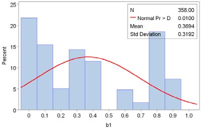
59 Figure 5.6 Regression Statistics of the Global Performance Models (distribution of regression coefficient, a) (distribution of regression coefficient, b) FDAC Original (distribution of regression coefficient, a) (distribution of regression coefficient, b) FDAC Heavy-Structural (distribution of regression coefficient, a) (distribution of regression coefficient, b) FDAC Light-Structural (distribution of regression coefficient, a) (distribution of regression coefficient, b) FDAC Non-Structural Cambridge Systematics, Inc. 5-11