Framing Lottery Choices

Transcription

1 Framing Lottery Choices by Dale O. Stahl Department of Economics University of Texas at Austin February 3, 2016 ABSTRACT There are many ways to present lotteries to human subjects: pie charts, vertical or horizontal bars, sometimes with numerical probabilities, sometimes with an indifference options. Unfortunately, the theories to be tested are silent on all these framing aspects. Expected Utility Theory (EUT) simply assumes that the decision maker has a complete understanding of the feasible payoffs and their respective probabilities, and can costlessly, instantaneously and errorlessly evaluate each lottery. We design and conduct an experiment which varies the framing of the lotteries in ways that lessen the cognitive difficulty of comparing lotteries. We find that as the ease of comparing lotteries increases, choice behavior becomes more consistent with EUT. 1

2 1. Introduction. The simplest case of a decision under risk is the choice between two objective lotteries. Indeed, theories about decisions under risk are typically developed first for these simple cases. Consequently, it is natural to test proposed theories with experiments that entail such choices. It is at the experimental design stage that we encounter many questions about how to present (or frame) the choices. 1 One common design is to present a lottery in the form of a pie chart: each section of the pie corresponds to a particular monetary payoff and the area of the section (as a percentage of the whole pie) is equal to the probability the lottery will yield that payoff. For a choice task, two pie charts are displayed on a computer screen side-by-side. Usually colors or distinctive shadings are used for specific payoffs. Sometimes, the numerical probabilities are listed below the pie chart. The choice screen also displays buttons to click (or keys to press) to make a choice. Sometimes an option of indifference is also available. 2 Unfortunately, the theories to be tested are silent on all these framing aspects. For instance, Expected Utility Theory simply assumes that the decision maker has a complete understanding of the lotteries (i.e. the feasible payoffs and their respective probabilities), and can costlessly, instantaneously and errorlessly evaluate each lottery. We do not have to be very cynical to question whether human subjects satisfy this auxiliary assumption in experiments when lotteries are presented as pie charts. Without numerical probabilities it is not easy to accurately assess the relative areas of the pie sections, and comparisons across the lotteries can be difficult due to the rotational orientation of the pies. Computing expected monetary values, let alone expected utilities, can be challenging to typical human subjects. Furthermore, the subjects almost surely have no experience with this specific or similar decision task, so they will not have a conceptual framework or useful heuristics to help them make the decision. They will find themselves in a situation similar to arriving in a foreign country with no knowledge of the local language and having to answer a question by the local customs official. 1 See Harrison and Rutström (2008) for a review of designs. 2 E.g. Hey and Orme (1994) and Harrison and Rutström (2009). 2

3 One of the main roles of college economics courses is to provide students with new concepts and a vocabulary to analyze economic choices. Therefore, we must recognize that lottery choice experiments test the joint hypotheses of an idealized theory and a complete and accurate understanding of the task and consequences by the subjects. When the latter understanding hypothesis is unlikely to hold, observations at odds with the joint hypotheses do not logically imply that the theory is false. Fortunately there are ways to exogenously vary the veracity of the understanding hypothesis, thereby partially unravelling the cause of the observed behavior. Specifically, we can change the presentation of the lotteries in ways that make the comparisons easier for the subjects. In this paper we report results from three presentation treatments. We start with a treatment that is similar to the standard framing to serve as a benchmark. The second treatment is essentially a rearrangement of the computer display that we believe makes it visually easier to compare the lotteries. The third treatment adds statements of facts about differences between the lotteries. To rule out learning across treatments, a subject participated in only one treatment. We find that each successive treatment results in less risk-averse behavior and an increase in risk-neutral behavior. We also want to infer any change in the proportion of the subjects who behave consistently with EUT. For this purpose, we estimate a two-parameter logistic choice function in which one parameter is for the utility function and the second parameter is for the precision. The lower the estimated precision, the more inconsistencies with EUT. We find a monotonic increase in the average precision, indicating fewer inconsistencies with EUT with the latter treatments. We believe it is important to recognize the heterogeneity in behavior in the subject population. Accordingly, we characterize the heterogeneity using a Bayesian method to estimate the distribution of the two parameters in the subject population (by treatment). Using this method, we estimate a dramatic increase in the proportion of the population that is behaviorally indistinguishable from risk-neutrality (i.e. maximize expected monetary value) from 12% to 45%. We also find no evidence of systematic fanning-out. 3

4 Section 2 presents the experimental design. Section 3 presents the analysis of the data. Section 4 concludes with a discussion. 2. The Experimental Design. We will first describe the lotteries that were used, and second the treatments. To avoid confounding effects from complicated lotteries, we chose lotteries with three possible outcomes: $5, $25, and $45. The lowest payoff was $5 instead of $0 to avoid the psychological effect of $0. This choice allows us to specify the utility function with just one parameter, such that U($5) = 0, U($45) = 1, and U($25) = u. Further, u = 0.5 represents risk neutrality. With three possible outcomes, lotteries can be represented as points in a Machina (1982) triangle. Figure 1 displays a Machina triangle with the lottery pairs shown as a line connecting two points (lotteries). For each pair, the one closest to the origin is the safe lottery, and the one closest to the diagonal boundary is the risky lottery. EUT implies that all indifference curves have slope u/(1-u). Whether EUT predicts choice of the safe or risky lottery depends solely u/(1-u). If the slope is less than u/(1-u), EUT predicts choice of the safe lottery, and if the slope is greater than u/(1-u), EUT predicts choice of the risky lottery. Since u can vary by subjects, we want to have lottery pairs with a variety of slopes. The slopes in our lottery pairs range from 0.5 to 4.0. To maximize the monetary incentive of each choice, we choose lotteries close to the safe origin and the diagonal boundary. The difference in the expected monetary value of the pairs ranged from $0 to $3, with an average of $2. Also to maximize the monetary incentive of each choice within our budget, we used 15 choices. While only 15 choices would be inadequate for some purposes, it suffices for our purpose. Moreover, there is a reasonable variety of pairs and instances of identical slopes to test for the EUT implication of parallel indifference curves. 4

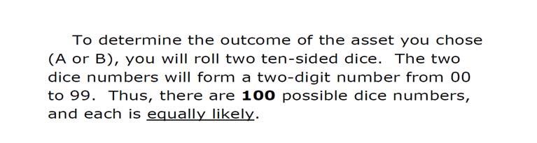
5 Figure 1. Lottery Pairs p p 5 All three treatments use sectioned horizontal bars to represent the lotteries with the sections ordered by increasing payoff. The $5 section was always colored pink; the $25 section was always colored yellow; and the $45 section was always colored blue. The length of each section as a proportion of the whole bar was exactly equal to the lottery s probability of the associated payoff. Figure 2. Representation of a Lottery The implementation of a lottery was described and carried out as follows. Two ten-sided dice are thrown: one blue die and one red die. The blue die counts 10s and the red die counts 1s. If the blue die is 6 and the red die is 3, the dice number is 63. All dice numbers from 00 to 99 are equally likely. Let pi (i = 5, 25, 45) denote the probability the lottery will yield payoff $5, 5

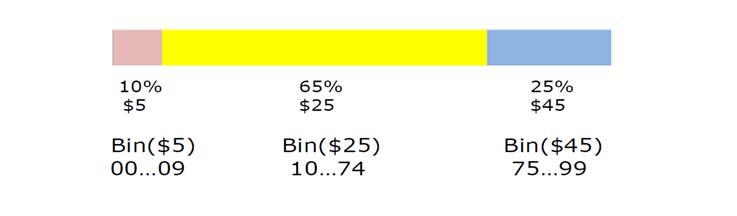
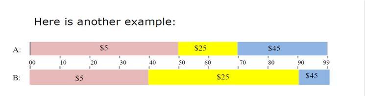
6 $25 and $45 respectively. If the dice number is less than p5, then the lottery will yield $5; if the dice number is greater than p5 but less than p5+p25, then the lottery will yield $25; if the dice number is greater than p5+p25, then the lottery will yield $45. We argue that this description and presentation is at least as understandable as the pie chart alternative. In the first treatment, two lotteries are displayed as side-by-side horizontal bars, comparable to side-by-side pie charts. Full instructions for each treatment are provided in Appendices A-C. In the second treatment, the horizontal bars are displayed one above the other. In addition each bar has a ruler line that runs from 00 to 99 corresponding to the possible dice numbers. In our opinion, it is much easier to compare the two lotteries in this stacked display. 3 For example, if lottery A pays $5 with probability 15%, and lottery B pays $5 with probability 25%, then it is fairly easy to see that both lotteries will pay $5 for all dice numbers from 00 to 14, and B will pay $20 more than A for dice number from 15 to 24. However, not all subjects may notice this, so we display these facts in a statement on the choice screen. It is possible that not all subjects recognize the usefulness of these facts. Therefore, we designed a third treatment in which the instructions focus the subjects attention on these facts via a short quiz, as well as also including in the Instructions 4 a statement of the form: because lottery A will pay $20 more than B for 35 dice numbers, and pay $20 less than B for 20 dice numbers, on average A will pay more than B. Obviously this additional statement is equivalent to informing the subjects about which lottery has the highest expected monetary value, but it does not suggest that maximizing expected monetary value is the right choice. 5 All subjects are free to consider the riskiness of each lottery. Indeed, risky lotteries stand out visually because the $25 payoff for a risky lottery corresponds to a much shorter (yellow) section of the bar. This visual saliency of the risk could discourage other comparisons. Moreover, the understanding 3 Camerer (1989), and Wakker, Erev and Webber (1994) utilized a similar display. 4 This statement is not displayed on the choice screens (see Appendix C). 5 Harrison and Rutström (2008) report that providing subjects with the expected monetary value of each lottery induces a sharp reduction in the estimated risk aversion. 6

7 hypothesis assumes that all subjects know the difference in expected monetary value. We argue that this third treatment makes the understanding hypothesis more likely to hold. Forty subjects participated in each treatment. The subjects were recruited from the general population of students at the University of Texas at Austin; however, graduate students in economics were not allowed to participate. An individual subject sat at a computer screen, read the instructions and made choices at their own pace. The experiment took from 10 to 30 minutes, and the average payoff was $ Analysis of the Data. a. Aggregate Percentage of Risky Choices A central hypothesis is that the proportion of risky lottery choices should increase with the slope ( p45/ p5) of the pair. Further, we expect the proportion also to increase with the treatment. Figure 3 displays the relevant aggregate data. In the legend, Tn stands for Treatment n. Figure 3. Percent Risky Lottery Choices T3 T2 T p 45 / p 5 7

8 Visually the data is consistent with our hypotheses for slopes greater than 1. That is, the curves are mostly upward sloping and each successive treatment shifts the curves upward for slopes greater than 1. A 3-by-12 ANOVA shows that the visual result is statistically significant at all common confidence levels. Detailed analysis of the treatment effect reveals that while the change from treatment 1 to treatment 3 is statistically significant, the change from treatment 1 to treatment 2 is not statistically significant at the 10% level. Since a EUT subject who is not riskloving will never choose a risky lottery when the slope is less than 1, the lack of any effect in this region can be attributed to the lack of risk-lovers in the subject pool. b. Mapping Behavior to EUT Model. The next question we want to address is how the framing treatment affects the likelihood that subjects behave according to EUT. Our first step is to map the observed behavior into a distribution over the two parameters of a simple logistic EUT model. Letting u U($25), the expected utility of a generic lottery is EU(p u) i {5,25,45} piui = p45 + (1- p5 p45)u. (1) Thus, given two lotteries p A and p B, the difference in expected utility is EU A,B (u) EU(p A u) - EU(p B u) = (1-u) p45 - u p5, (2) where p45 = (p45 p45), etc. A B Letting be the precision of the logistic choice, the probability of choosing lottery p A over p B is P(u, ) 1/[1 + exp{- EU A,B (u)}]. (3) 8

9 Obviously, the probability of choosing lottery p B over p A is 1 - P(u, ). Given a subject s 15 choices, we can calculate the likelihood of those choices as a function of (u, ) by computing the product of the probabilities for each choice. Provided we are willing to assume a prior on (u, ), we can compute a Bayesian posterior distribution on (u, ). In other words, we can map the behavior into a distribution on parameters of the logistic EUT model. Moreover, assuming the subjects are random draws from a common subject pool, we can refine the posterior distribution. Adopting the method of Stahl (2014, 2015), briefly described in Appendix D, we compute the posterior distribution of (u, ) for the population of subjects for each treatment. Figure 3 displays the results. 9

10 Figure 3. Population Distribution of (u, ) by Treatment u p( ) (a) Treatment u p( ) 10

11 (b) Treatment u p ) (c) Treatment 3 The vertical scales are the same for all three graphs to facilitate comparisons. Instead of on the depth axis, we plot p( ) 1/[1 + exp(-0.05 )], which translates into the behavioral probability that an option with a 5% greater value will be chosen. The visual differences between these graphs is dramatic. With treatment 1, the posterior is diffuse and spread over low precisions and u > 0.5, which is consistent with the common finding that subjects appear to be risk averse and that EUT does not fit behavior well. Moving to treatment 2, we see a decrease in high values of u (risk-aversion) and two small spikes at high precisions. This observation suggests that the stacked bars did facilitate comparisons for some subjects thereby increasing their consistency. 11

12 With treatment 3, we see a dramatic spike near u = 0.5 and p = 1, which represents the risk-neutral EU maximizer. We also observe a further decrease in the spread over u. Table 1 shows the mean and standard deviation of the distribution by treatment. Table 1. Mean and Standard Deviation by Treatment Treatment 1 Treatment 2 Treatment 3 u (0.161) (0.122) (0.126) p( ) (0.112) (0.120) (0.124) Clearly the mean u decreases and the mean p( ) increases with the treatment. c. Shifts in Probability Mass by Treatment. Our next objective is to use the posterior distributions to discern the shift in probability mass towards the risk-neutral EUT model with treatment. To do this, we need the concept of behaviorally distinguishable parameters. To assess whether our data (xi) was generated by (u, ) or (u, ), we typically compute the log-likelihood ratio (LLR): ln[f(xi u, )/f(xi u, )]. However, it is well-known that likelihood-ratio tests are subject to type-i and type-ii errors. We define (u, ) to be behaviorally indistinguishable from (u, ), if either of the type-i and type-ii error rates 6 exceed 10%, and to be behaviorally distinguishable if both of the type-i and type-ii error rates are less than or equal to 10%. To begin, we want to know what percent of the population is behaviorally indistinguishable from 50:50 random choices (hereafter referred to as Level-0 or L0 behavior). Since the latter entails the simple restriction that = 0, we can compute whether (u, ) is behaviorally indistinguishable from (u, 0), and then integrate the posterior over all the points (u, ) that are behaviorally indistinguishable from (u, 0). We do this for each treatment and report the results in the first row of Table 2. It is curious that Treatment 2 produces the largest mass of Level-0 behavior. One possible explanation is that there was some learning by doing (even 6 These rates can be computed exactly since there are only 2 15 possible 15-tuples of choice data for an individual subject. For details, see Stahl (2014, 2015). 12

13 without feedback) which manifests itself as inconsistent behavior, whereas the quiz in Treatment 3 induced similar learning before the choices were made. Table 2. Posterior Probability of Hypotheses Treatment 1 Treatment 2 Treatment 3 Level Not L0 & u= Not L0 & u EMV* The second computation of interest is the probability mass that is behaviorally distinguishable from Level-0 but indistinguishable from risk-neutrality: i.e. the integral of the posterior over all the points (u, ) that are behaviorally indistinguishable from (0.5, ). These results are reported in the second row of Table 2. Clearly, Treatment 3 more than doubles the amount of risk-neutral behavior. The third row of Table 2 is calculated as 1.0 minus the sum of the first two rows. Thus, the numbers in this row are the probability mass that is behaviorally distinguishable from Level=0 and behaviorally distinguishable from risk-neutrality. This mass decreases substantially from treatment 1 to treatment 3. The third and final computation of interest is the probability mass that is behaviorally indistinguishable from very precise maximization of EMV: i.e. the integral of the posterior over all the points (u, ) that are behaviorally distinguishable from Level=0 but behaviorally indistinguishable from (0.5, 138) 7. These results are reported in the fourth row of Table 2. Clearly, Treatment 3 produces the largest mass of very precise maximization of EMV. Moreover, the proportions of those who are risk neutral but not Level-0 (second row of Table 2), and who are very precise (fourth row) by treatment are 0.391, and respectively. 8 In 7 p(138) = 0.999, so choosing the inferior lottery when the difference in expected value is 5% would happen only 1 out of 1000 times; hence, we consider this very high precision. 8 Row 4 divided by row 2. 13

14 other words, Treatment 3 also produces a significant increase in the precision of the risk-neutral types. d. Common Ratio Tests. In the design there are three p45/ p5 slope values that occurred twice: (3, 2 and 0.5). One occurrence entailed lottery pairs that were in the northwest area of Figure1, and the other entailed lottery pairs that were in the southeast area of Figure 1. These pairs allow us to test the common ratio implication of EUT: that the choices in each occurrence with a common slope should be both risky or both safe. The Allais paradox is the classic example of failure of this prediction. In the Allais paradox, one lottery pair is in the northwest area of Figure 1 and the other pair is in the southeast area. The typical finding is that subjects choose the safe lottery from the northwest pair and the risky lottery from the southeast pair. This behavior suggests a fanning out of the indifference curves such that U($25) is larger for the northwest pair than for the southwest pair, as if subjects were more risk averse when the expected value is high. 9 Table 3 displays the number of switches from safe to risky (S to R) and vice versa. Table 3. Common Ratio Results Treatment 1 Treatment 2 Treatment 3 S to R R to S Total % EUT Since EUT predicts no switching (although the logistic choice model allows switching as an idiosyncratic error), the total number of switches (out of 120 possible) indicates the possible violations of EUT. The number of switches decreases with treatment, and with Treatment 3, 83.3% of all choices are consistent with EUT (i.e. no switches). Curiously, we find essentially 9 See Machina (1982, 1987). 14

15 the same number of R to S switches as S to R switches. Thus, the fanning out hypothesis is no more likely than the contrary fanning in hypothesis. It seems more plausible that these switches are idiosyncratic errors rather than a manifestation of non-eut preferences. These findings are consistent with Kagel, et al. (1990). 4. Conclusions. We designed three presentation treatments for binary lottery experiments. The treatments systematically increased ease of comparing the lotteries. As anticipated, with increased ease of comparison, behavior became more consistent with EUT. More risky choices were made, and the mean measure of risk-aversion decreased from 0.7 to 0.6. Further, behavior became more precise, which can be interpreted as the influence of the fundamentals increasing relative to idiosyncratic features, inattention or noise. Moreover, the proportion of behavior that was consistent with maximizing expected monetary value went from 12% to 45%. Finally, we found no evidence for the fanning out hypothesis that is used to explain the Alais paradox. Clearly, framing effects are significant. Therefore, observed behavior that appears to be inconsistent with EUT may actually be driven by obscure framing of the choice. Of course, outside the laboratory, choices are often obscurely framed, so it would be premature to predict EUT behavior for those choices. On the other hand, when stakes are high and experience has provided useful tools of comparison, EUT may perform well. 15

16 References Camerer, C. (1989). An experimental test of several generalized utility theories, J. of Risk and Uncertainty, 2, Harrison, G. (1989). Theory and Misbehavior of First-Price Auctions, Am. Econ. Rev., 79, Harrison, G. (1992). Theory and Misbehavior of First-Price Auctions: Reply, Am. Econ. Rev., 82, Harrison, G., and Rutström, E. (2008). Risk Aversion in the Laboratory, In J. C. Cox and G. W. Harrison, eds., Research in Experimental Economics, 12, Harrison, G., and Rutström, E. (2009). Expected Utility and Prospect Theory: One Wedding and Decent Funeral, Experimental Economics, 12, Hey, J., and Orme, C. (1994). Investigating Generalizations of Expected Utility Theory Using Experimental Data, Econometrica, 62, Kagel, J., MacDonald, D., and Battalio, R. (1990). "Tests of `Fanning Out of Indifference Curves: Results from Animal and Human Experiments American Economic Review, 80, Machina, M. (1982). 'Expected Utility' Analysis Without the Independence Axiom, Econometrica, 50, Machina, M. (1987). Choice Under Uncertainty: Problems Solved and Unsolved," Journal of Economic Perspectives, 1, Stahl, D. (2014). Heterogeneity of Ambiguity Preferences, Rev. of Econ. and Statistics, 96, Stahl, D. (2015)."Re-examination of Experiment Data on Lottery Choices," working paper. Wakker, P., Erev, I., and Weber, E. (1994). Comonotonic independence: The critical test between classical and rank-dependent utility theories, J. of Risk and Uncertainty, 9,

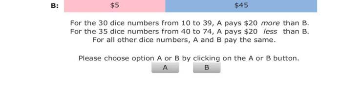
17 APPENDIX A Instructions for Treatment 1 Pg 1: Welcome. This is an experiment about economic decision making in which you are asked to make 15 choices. Each choice will be between two assets whose dollar returns have different levels of uncertainty. You may take as much time as you need to make your 15 choices. After you have made your choices, the uncertainty about the return to the assets you chose will be resolved by the roll of dice. When you conclude, you will be paid in cash an amount that depends on the choices you made, and on the outcomes of the dice rolls. Earnings can range from $5 to $45. Pg 2: Pg 3: 1

18 Pg 4: 2

19 Pg 5: Pg 6: 3

20 Pg 7: 4

21 Pg 8: 5

22 APPENDIX B Instructions for Treatment 2 Pages 1-2 are the same as in Treatment 1. Pg 3: Pg 4: Pg 5: 6

23 Demo Screen: Pg 6: Pg 7: 7

24 APPENDIX C Instructions for Treatment 3 Page 1 is the same as in Treatments 1 and 2. Pg 2: Pg 3: 8

25 Pg 4: Pg 5: Pg 6: 9

26 Pg 7: 10

27 Pg 8: Demo Screen: Pg 9: 11

28 Pg 10: 12

29 APPENDIX D: Method Used to Produce Figure 3. Let xi denote the choice data for subject i, and let f(xi ) denote the probability of xi given parameter vector (, u). Given a prior g0 on, by Bayes rule, the posterior on is g( xi) f(xi )g0( )/ f(xi z)g0(z)dz. (D1) However, eq(d1) does not use information from the other subjects even though those subjects were randomly drawn from a common subject pool. Let N be the number of subjects in the data set. When considering subject i, it is reasonable to use as a prior, not g0, but gi( ) 1 N 1 h i g( xh) (D2) In other words, having observed N-1 subjects, gi( ) is the probability that the N th random draw from the subject pool will have parameter vector. We then compute ĝ i ( x) f(xi )gi( )/ f(xi z)gi(z)dz, (D3) where x denotes the entire N-subject data set. Finally, we aggregate these posteriors to obtain 1 N g*( x) ĝ i 1 i ( x). (D4) N We can interpret g*( x) as the probability density that a random draw from the subject pool will have parameter vector. When implementing this method we specified the prior g0 as follows. For the logit precision parameter, we specify = 20ln[p/(1-p)] with p uniform on [0, 0.999]. In this formulation, p can be interpreted as the probability an option with a 5% greater value will be chosen. u is uniform on [0, 1]. These two distributions are assumed to be independent. For computations, we used a grid of 41x41points.