FIGURE A1.1. Differences for First Mover Cutoffs (Round one to two) as a Function of Beliefs on Others Cutoffs. Second Mover Round 1 Cutoff.

Transcription

1 APPENDIX A. SUPPLEMENTARY TABLES AND FIGURES A.1. Invariance to quantitative beliefs. Figure A1.1 shows the effect of the cutoffs in round one for the second and third mover on the best-response cutoffs for the first mover in round two. In particular the figure indicates the difference in best response between the first and second round, so 51 µ 1,2 (µ 2,1, µ 2,3 ). For most second- and third-mover responses close to the equilibrium the best response is identical. Even with substantially different beliefs about the cutoffs, the first mover should still have a difference in their first and second cutoffs of at least 10. The sole exceptions are those cases where the second and third movers are believed to use boundary cutoffs, either always or never switching. FIGURE A1.1. Differences for First Mover Cutoffs (Round one to two) as a Function of Beliefs on Others Cutoffs Always (100) Second Mover Round 1 Cutoff μ (51) μ * 2,1 (42) Difference of Never (1) Never (1) * μ 3,1 (35) μ (51) Always (100) Third Mover Round 1 Cutoff 1

2 A.2. Experimental Design. Overall allocation of subjects to session is given in Table A2.1. Treatment Type Sessions Subjects Supergames Selection Game ,386 No Selection Decision S-Across Game ,260 S-Within Game ,446 S-Explicit Decision S-Peer Game ,512 S-Simple-Random Game ,952 S-Simple-Fixed Game ,952 All ,960 FIGURE A2.1. Experimental Design Table 2

3 A.3. Robustness. This appendix contains tables and figures that extend the analysis in the main text. Table A3.1 reports the same regressions as in Table 1 in the main text, but using data from supergames 6 to 20 instead of supergames 11 to 20. Table A3.2 extends the same analysis for players in the role of second- and third-movers, and finds very similar results. Table A3.3 replicates the analysis from Table 1 for the S-Across treatment, and Table A3.4 extends the analysis to include data from supergames 6 to 20. Tables A3.5 and A3.6 do the same for the S-Explicit treatment. Table A3.7 report results from the S-Within treatment, in which subjects are informed about the actions taken by other players during the course of the supergame. In the S- Within treatment, the relevant conditioning variable should be the information that other people switched, and the passing of time per se does not convey direct actionable information. Table A3.8 extends the analysis to include data from supergames 6 to 20. Tables A3.9 and A3.10 report results of supergame 21 behavior for subjects in the S- Within and S-Peer treatments, respectively. For both cases, we cannot reject the hypothesis that cutoffs are similar to the Selection treatment. We conclude that neither receiving strategic feedback during the path of play, nor discussing the optimal strategy with peers significantly affects behavior in supergame 21. 3

4 TABLE A3.1. Average Cutoff per Round for No Selection and Selection Treatments, First-Movers Only Treatment Game Round Theory Supergame 6 to 20 Supergame 21 Estimate Test (p-value) Estimate Test (p-value) No Selection (Control) µ ˆµ ˆµ j t = ˆµ NS 1 ˆµ j t = µ j t ˆµ ˆµ j t = ˆµ NS 1 ˆµ j t = µ j t Round 1, ˆµ NS 1 [51] (2.40) (2.48) Round 2, ˆµ NS 2 [51] (2.42) (2.48) Round 3, ˆµ NS 3 [51] (2.46) (2.48) Joint Tests: Selection (Treatment) Round 1, ˆµ S 1 [51] (1.20) (3.04) Round 2, ˆµ S 2 [35] (1.23) (3.04) Round 3, ˆµ S 3 [28] (1.30) (3.04) Joint Tests: Note: Figures derived from a single random-effects least-squares regression for all chosen cutoffs against treatment-round dummies. Standard errors in parentheses, risk-neutral predicted cutoffs in square brackets (switch ball if value is lower than cutoff). There are 171/138/33 Total/Selection/No Selection first-mover subjects across supergames 6-20, and 55/22/33 in supergame 21. Selection treatment exclude subjects in the second- and third-mover roles. Univariate significance tests columns examine differences from either the first-round coefficient from the control (H0 :ˆµ j t = ˆµ NS 1 for treatment j, round t) and the theoretical prediction (H0 :ˆµ j t = µ j t ). Joint test of stationary cutoffs across the supergame (H0 : ˆµ j 1 = ˆµj 2 = ˆµj 3 (H0 : 0 = ˆµ j 1 µ j 1 = ˆµj 2 µ j 2 = ˆµj 3 µ j 3 ). for treatment j); Joint test of PBE cutoffs in supergame 4

5 TABLE A3.2. Average Cutoff per Round for Selection Treatments, Second- and Third-Movers Treatment Game Round Theory Supergame 11 to 20 Supergame 21 Estimate Test (p-value) Estimate Test (p-value) Selection, Second-Movers µ ˆµ ˆµ j t = ˆµ NS 1 ˆµ j t = µ j t ˆµ ˆµ j t = ˆµ NS 1 ˆµ j t = µ j t Round 1, ˆµ S 1 [42] (0.68) (2.80) Round 2, ˆµ S 2 [31] (0.98) (2.80) Round 3, ˆµ S 3 [25] (1.40) (2.80) Joint Tests: Selection, Third-Movers Round 1, ˆµ S 1 [35] (1.31) (2.57) Round 2, ˆµ S 2 [28] (1.34) (2.57) Round 3, ˆµ S 3 [23] (1.40) (2.57) Joint Tests: Note: Figures derived from a single random-effects least-squares regression for all chosen cutoffs against treatment-round dummies. Standard errors in parentheses, risk-neutral predicted cutoffs in square brackets (switch ball if value is lower than cutoff). There are 133/138 second-/third-mover subjects across supergames 11-20, and 22 second- and third-movers in supergame 21. Univariate significance tests columns examine differences from either the first-round coefficient from the control (H0 :ˆµ j t = ˆµ NS 1 for treatment j, round t) and the theoretical prediction (H0 :ˆµ j t = µ j t ). Joint test of stationary cutoffs across the supergame (H0 : ˆµ j 1 = ˆµj 2 = ˆµj 3 test of PBE cutoffs in supergame (H0 : 0 = ˆµ j 1 µ j 1 = ˆµj 2 µ j 2 = ˆµj 3 µ j 3 ). for treatment j); Joint 5

6 TABLE A3.3. Average Cutoff per Round for S-Across Treatment, First-Movers Only Treatment Game Round Theory Supergame 11 to 20 Supergame 21 Estimate Test (p-value) Estimate Test (p-value) S-Across µ ˆµ ˆµ j t = ˆµ NS 1 ˆµ j t = ˆµ S t µ j t = µ j t ˆµ ˆµ j t = ˆµ NS 1 ˆµ j t = ˆµ S t ˆµ j t = µ j t Round 1, ˆµ S(A) 1 [51] (1.93) (3.31) Round 2, ˆµ S(A) 2 [35] (2.00) (3.31) Round 3, ˆµ S(A) 3 [28] (2.11) (3.31) Joint Tests: Note: Figures derived from a single random-effects least-squares regression for all chosen cutoffs against treatment-round dummies. Standard errors in parentheses, risk-neutral predicted cutoffs in square brackets (switch ball if value is lower than cutoff). There are 60 first-mover subjects across supergames 11-20, and 20 first-movers in supergame 21. Univariate significance tests columns examine differences from either the first-round coefficient from the control (H0 :ˆµ j t = ˆµ NS 1 for treatment j, round t), the first-mover coefficients from the Selection treatment (H0 :ˆµ j t = ˆµ S t for treatment j, round t) and the theoretical prediction (H0 :ˆµ j t = µ j t ). Joint test of stationary cutoffs across the supergame (H0 : ˆµ j 1 = ˆµj 2 = ˆµj 3 for treatment j); Joint test of PBE cutoffs in supergame (H 0 : 0 = ˆµ j 1 µ j 1 = ˆµj 2 µ j 2 = ˆµj 3 µ j 3 ). 6

7 TABLE A3.4. Average Cutoff per Round for S-Across Treatment, First-Movers Only Treatment Game Round Theory Supergame 6 to 20 Supergame 21 Estimate Test (p-value) Estimate Test (p-value) S-Across µ ˆµ ˆµ j t = ˆµ NS 1 ˆµ j t = ˆµ S t µ j t = µ j t ˆµ ˆµ j t = ˆµ NS 1 ˆµ j t = ˆµ S t ˆµ j t = µ j t Round 1, ˆµ S(A) 1 [51] (1.90) (3.31) Round 2, ˆµ S(A) 2 [35] (1.94) (3.31) Round 3, ˆµ S(A) 3 [28] (2.02) (3.31) Joint Tests: Note: Figures derived from a single random-effects least-squares regression for all chosen cutoffs against treatment-round dummies. Standard errors in parentheses, risk-neutral predicted cutoffs in square brackets (switch ball if value is lower than cutoff). There are 60 first-mover subjects across supergames 6-20, and 20 first-movers in supergame 21. Univariate significance tests columns examine differences from either the first-round coefficient from the control (H0 :ˆµ j t = ˆµ NS 1 for treatment j, round t), the first-mover coefficients from the Selection treatment (H0 :ˆµ j t = ˆµ S t for treatment j, round t) and the theoretical prediction (H0 :ˆµ j t = µ j t ). Joint test of stationary cutoffs across the supergame (H0 : ˆµ j 1 = ˆµj 2 = ˆµj 3 for treatment j); Joint test of PBE cutoffs in supergame (H 0 : 0 = ˆµ j 1 µ j 1 = ˆµj 2 µ j 2 = ˆµj 3 µ j 3 ). 7

8 TABLE A3.5. Average Cutoff per Round for S-Explicit Treatment Treatment Game Round Theory Supergame 11 to 20 Supergame 21 Estimate Test (p-value) Estimate Test (p-value) S-Explicit µ ˆµ ˆµ j t = ˆµ NS 1 ˆµ j t = ˆµ S t µ j t = µ j t ˆµ ˆµ j t = ˆµ NS 1 ˆµ j t = ˆµ S t ˆµ j t = µ j t Round 1, ˆµ S(E) 1 [51] (2.47) (4.55) Round 2, ˆµ S(E) 2 [34] (2.49) (4.55) Round 3, ˆµ S(E) 3 [17] (2.55) (4.55) Joint Tests: Note: Figures derived from a single random-effects least-squares regression for all chosen cutoffs against treatment-round dummies. Standard errors in parentheses, risk-neutral predicted cutoffs in square brackets (switch ball if value is lower than cutoff). There are 36 subjects in the S-Explicit treatment across supergames 11-20, and 12 first-movers in supergame 21. Univariate significance tests columns examine differences from either the first-round coefficient from the control (H0 :ˆµ j t = ˆµ NS 1 for treatment j, round t), the firstmover coefficients from the Selection treatment (H0 :ˆµ j t = ˆµ S t for treatment j, round t) and the theoretical prediction (H0 :ˆµ j t = µ j t ). Joint test of stationary cutoffs across the supergame (H0 : ˆµ j 1 = ˆµj 2 = ˆµj 3 (H0 : 0 = ˆµ j 1 µ j 1 = ˆµj 2 µ j 2 = ˆµj 3 µ j 3 ). for treatment j); Joint test of PBE cutoffs in supergame 8

9 TABLE A3.6. Average Cutoff per Round for S-Explicit Treatment Treatment Game Round Theory Supergame 6 to 20 Supergame 21 Estimate Test (p-value) Estimate Test (p-value) S-Explicit µ ˆµ ˆµ j t = ˆµ NS 1 ˆµ j t = ˆµ S t µ j t = µ j t ˆµ ˆµ j t = ˆµ NS 1 ˆµ j t = ˆµ S t ˆµ j t = µ j t Round 1, ˆµ S(E) 1 [51] (2.42) (4.55) Round 2, ˆµ S(E) 2 [34] (2.44) (4.55) Round 3, ˆµ S(E) 3 [17] (2.48) (4.55) Joint Tests: Note: Figures derived from a single random-effects least-squares regression for all chosen cutoffs against treatment-round dummies. Standard errors in parentheses, risk-neutral predicted cutoffs in square brackets (switch ball if value is lower than cutoff). There are 36 subjects in the S-Explicit treatment across supergames 6-20, and 12 first-movers in supergame 21. Univariate significance tests columns examine differences from either the first-round coefficient from the control (H0 :ˆµ j t = ˆµ NS 1 for treatment j, round t), the firstmover coefficients from the Selection treatment (H0 :ˆµ j t = ˆµ S t for treatment j, round t) and the theoretical prediction (H0 :ˆµ j t = µ j t ). Joint test of stationary cutoffs across the supergame (H0 : ˆµ j 1 = ˆµj 2 = ˆµj 3 (H0 : 0 = ˆµ j 1 µ j 1 = ˆµj 2 µ j 2 = ˆµj 3 µ j 3 ). for treatment j); Joint test of PBE cutoffs in supergame 9

10 TABLE A3.7. Average Cutoff per Round and Number of In-Group Switches, S-Within Treatment Treatment In-Group Switches Theory Supergame 11 to 20 S-Within Estimates µ Round 1, ˆµ S(W ) 1s Round 2, ˆµ S(W ) 2s Round 3, ˆµ S(W ) 3s Joint Te Zero [51] [0.000] [0.000] [0.000] (1.80) (1.87) (2.03) One [14] [0.000] [0.000] [0.000] (1.88) (1.87) (1.95) Two [3] [0.000] [0.000] [0.000] (2.76) (2.25) (2.26) Joint Tests: Note: Figures derived from a single random-effects least-squares regression for all chosen cutoffs against treatment-round dummies. Standard errors in parentheses, risk-neutral predicted cutoffs in square brackets (switch ball if value is lower than cutoff). There are 69 subjects across supergames P-Value of univariate significance tests of the theoretical predictions (H 0 :ˆµ j ts = µ j ts ). Join test: Cutoffs are stationary across the treatment (H 0 : ˆµ S(W ) 1s = ˆµ S(W ) 2s = ˆµ S(W ) 3s across rounds, and H 0 : ˆµ S(W ) t1 = ˆµ S(W ) t2 = ˆµ S(W ) t3 across number of in-group switches). 10

11 TABLE A3.8. Average Cutoff per Round and Number of In-Group Switches, S-Within Treatment Treatment In-Group Switches Theory Supergame 6 to 20 S-Within Estimates µ Round 1, ˆµ S(W ) 1s Round 2, ˆµ S(W ) 2s Round 3, ˆµ S(W ) 3s Joint Te Zero [51] [0.000] [0.000] [0.000] (1.68) (1.72) (1.86) One [14] [0.000] [0.000] [0.000] (1.73) (1.72) (1.79) Two [3] [0.000] [0.000] [0.000] (2.45) (2.05) (2.06) Joint Tests: Note: Figures derived from a single random-effects least-squares regression for all chosen cutoffs against treatment-round dummies. Standard errors in parentheses, risk-neutral predicted cutoffs in square brackets (switch ball if value is lower than cutoff). There are 69 subjects across supergames P-Value of univariate significance tests of the theoretical predictions (H 0 :ˆµ j ts = µ j ts ). Join test: Cutoffs are stationary across the treatment (H 0 : ˆµ S(W ) 1s = ˆµ S(W ) 2s = ˆµ S(W ) 3s across rounds, and H 0 : ˆµ S(W ) t1 = ˆµ S(W ) t2 = ˆµ S(W ) t3 across number of in-group switches). 11

12 TABLE A3.9. Average Cutoff per Round in Supergame 21 for S-Within Treatment, First-Movers Only Treatment Game Round Theory Supergame 21 S-Within Estimate Test (p-value) µ ˆµ ˆµ j t = ˆµ NS 1 ˆµ j t = ˆµ S t ˆµ j t = µ j t Round 1, ˆµ S(W ) 1 [51] (3.32) Round 2, ˆµ S(W ) 2 [35] (3.32) Round 3, ˆµ S(W ) 3 [28] (3.32) Joint Tests: Note: Figures derived from a single random-effects least-squares regression for all chosen cutoffs against treatment-round dummies. Standard errors in parentheses, risk-neutral predicted cutoffs in square brackets (switch ball if value is lower than cutoff). There are 23 first-mover subjects in supergame 21. Univariate significance tests columns examine differences from either the first-round coefficient from the control (H 0 :ˆµ j t = ˆµ NS 1 for treatment j, round t), the first-mover coefficients from the Selection treatment (H 0 :ˆµ j t = ˆµ S t for treatment j, round t) and the theoretical prediction (H 0 :ˆµ j t = µ j t ). Joint test of stationary cutoffs across the supergame (H 0 : ˆµ j 1 = ˆµj 2 = ˆµj 3 for treatment j); Joint test of PBE cutoffs in supergame (H 0 : 0 = ˆµ j 1 µ j 1 = ˆµj 2 µ j 2 = ˆµj 3 µ j 3 ). 12

13 TABLE A3.10. Average Cutoff per Round for S-Peer Treatment on Supergame 21, First-Movers Only Treatment Game Round Theory Supergame 21 S-Peer Estimate Test (p-value) µ ˆµ ˆµ j t = ˆµ NS 1 ˆµ j t = ˆµ S t ˆµ j t = µ j t Round 1, ˆµ S(A) 1 [51] (3.31) Round 2, ˆµ S(A) 2 [35] (3.31) Round 3, ˆµ S(A) 3 [28] (3.31) Joint Tests: Note: Figures derived from a single random-effects least-squares regression for all chosen cutoffs against treatment-round dummies. Standard errors in parentheses, risk-neutral predicted cutoffs in square brackets (switch ball if value is lower than cutoff). There are 24 first-mover subjects in supergame 21. Univariate significance tests columns examine differences from either the first-round coefficient from the control (H 0 :ˆµ j t = ˆµ NS 1 for treatment j, round t), the first-mover coefficients from the Selection treatment (H 0 :ˆµ j t = ˆµ S t for treatment j, round t) and the theoretical prediction (H 0 :ˆµ j t = µ j t ). Joint test of stationary cutoffs across the supergame (H 0 : ˆµ j 1 = ˆµj 2 = ˆµj 3 for treatment j); Joint test of PBE cutoffs in supergame (H 0 : 0 = ˆµ j 1 µ j 1 = ˆµj 2 µ j 2 = ˆµj 3 µ j 3 ). 13

14 TABLE A3.11. Average Cutoff in Last Round for Within and Between Treatments (Supergame 40) Treatment Game Round Theory Between Within Estimate p-values Estimate p-values Within µ ˆµ H0 : ˆµ W j = ˆµ W 1 H0 : ˆµ j t = µ j t ˆµ H0 : ˆµ j t = ˆµ NS 1 H0 : ˆµ j t = µ j t Round 1, ˆµ NS 1 [51] (2.85) (2.85) Round 2, ˆµ NS 2 [32] (2.85) (2.85) Round 3, ˆµ NS 3 [22] (2.85) (2.85) Joint Tests: Note: Figures derived from a single OLS regression (N = 144 subjects each making a single choice) against treatment-round dummies. Standard errors in parentheses, risk-neutral predicted cutoffs in square brackets (switch ball if value is lower than cutoff). Univariate significance tests columns examine differences from either the first-round coefficient from the control (H0 :ˆµ j t = ˆµ NS 1 for treatment j, round t), the first-mover coefficients from the Selection treatment (H0 :ˆµ j t = ˆµ S t for treatment j, round t) and the theoretical prediction (H0 :ˆµ j t = µ j t ). Joint test of stationary cutoffs across the supergame (H0 : ˆµ j 1 = ˆµj 2 = ˆµj 3 supergame (H0 : 0 = ˆµ j 1 µ j 1 = ˆµj 2 µ j 2 = ˆµj 3 µ j 3 ). for treatment j); Joint test of PBE cutoffs in 14

15 1.0 Type Proportion Allowed Type Error (A) Selection 1.0 Type Proportion Stationary Decreasing Other Allowed Type Error (B) No Selection FIGURE A4.1. Type Robustness to ɛ A.4. Type Classification Robustness. In Figure A4.1 we indicate the three type categories as we vary the bandwidth parameter ɛ from 0 to 10. Table A4.1 reports on the proportion of types as classified in the last five partial strategy supergames for each treatment. Rather than the full strategy method final supergames, we here take averages across supergames to assess the strategy cutoffs. Following the paper we focus on the type specifications with an error bandwidth ɛ = 2.5 (though we also provide data on ɛ = 0 and ɛ = 5). For treatment S-Simple-Random a subject is decreasing if the difference in average cutoffs for all pairwise comparisons (first minus second-mover, first minus third-mover, and 15

16 second minus third-mover) are strictly positive; likewise, subject is ɛ-decreasing if all such differences are (weakly) greater than ɛ. For treatment S-Within subject is decreasing if the difference in average cutoffs for all pairwise comparisons (no switches minus 1 switch, no switches minus 2 switches, and 1 switch minus 2 switches) are strictly positive; and subject is ɛ-decreasing if all such differences are (weakly) greater than ɛ. For all other treatments subject is decreasing if minimum of (round 1 - round 2) cutoffs, irrespective of type, is strictly positive, and is ɛ-decreasing if minimum is larger than ɛ. Treatment Selection includes data from S-Deliberation as both treatment are identical up until cycle

17 TABLE A4.1. Type Classifications on Last Five Cycles NS Decreasing Non-Decreasing Total Stationary Exact ɛ = 2.5 ɛ = 5 Exact ɛ = 2.5 ɛ = 5 Exact ɛ = 2.5 ɛ = 5 No Selection % 30.3% 15.2% 48.5% 69.7% 84.8% 48.5% 69.7% 72.7% Selection % 26.1% 24.6% 69.6% 73.9% 75.4% 34.8% 47.8% 53.6% 17 S-Across % 50% 36.7% 38.3% 50% 63.3% 38.3% 45% 51.7% S-Explicit % 61.1% 41.7% 19.5% 38.9% 58.3% 19.5% 30.6% 36.1% S-Within % 55.1% 50.7% 30.4% 44.9% 49.3% 24.6% 42% 46.4% S-Simple-Random % 40.3% 34.7% 51.4% 59.7% 65.3% 26.4% 43.1% 55.6% Note: Type classification based on cutoffs chosen in cycles for S-Simple-Random and cycles for all other treatments.

18 TABLE A5.1. Individual Regressions Explanatory Variables (I) (II) (III) Sel. Only Sel.+NoSel. Sel.+NoSel. Experienced Rematching ˆν 1,10 G ˆν 11,20 G Experienced Outcomes ˆν 1,10 H ˆν 11,20 H Risk Aversion ˆρ No Selection δ NoSel Constant N R Note: Statistically significant variables indicated by stars ( 10%; 5%; 1%) with p-values beneath them. R 2 is the adjusted R-squared measure of fit. A.5. Effects from Experience and Risk Aversion. For each ɛ-stationary subject we generate their experienced rematching (ˆν i G ) and final (ˆν i H ) outcomes, averaging across supergames 1 10 and supergames Despite facing the same generating process in each treatment there is substantial subject variation in rematching and final outcomes in these blocks of ten supergames. For each individual subject variation in the average experiences can be used to validate the mechanic in the hypothesized learning model. In Table A5.1, we regress each stationary subject s supergame-21 cutoff choice on the observed experiences (ˆν i G and ˆν i H ) and elicited risk preference (ˆρ i ). In the first regression (Column I), we present results for the 66 stationary-type subjects in our Selection treatments (the baseline and S-Across). In the second (Column II) we pool in the additional 25 stationary subjects from the No Selection treatment (including a treatment dummy). In the third regression, we remove the experienced rematching (both) and late-session experienced final outcomes as independent variables (which can be motivated by the adjusted R-squared measures provided in the last row). Across specifications we find that variation in final outcomes in the early-session supergames, ˆν 1,10, H has a strong effect in the predicted direction. However, subjects learning seems to occur quite quickly, as we do not find a significant final cutoff response to final-outcome variation in the second block of ten supergames. While the signs on both rematching variables and the late-session final-outcome variable are positive, the size of the estimated effects are far smaller than for the early-session final outcomes. Separate from experience, subject-variation in elicited risk preferences is a significant predictor for 18

19 subjects final supergame cutoffs in all of the regressions, reflecting the other requirement for the aggregate match made by the behavioral model. 19

20 Appendix B. Theoretical Model We model a dynamic setting with adverse selection occurring over time. To do this we set up a finite population of objects O = {o 1,..., o M } (with the interpretation of longside participants or durable goods, etc.). Each object has a common value, an iid draw over V R according to a commonly known distribution F so that the average value is v. These objects are initially matched to a group of individuals I = {1,..., N} (with the interpretation of short-side participants, consumers, etc.). Each individual is randomly assigned to one of the objects at the beginning of the game through a one-to-one matching function, so that individual i has the initial object µ i 0. In our setting there are more objects than individuals (N < M) and so some of the objects Ô0 O are initially unassigned. The set of unassigned objects will function here as a rematching population, and it is adverse selection over this population that is our main focus. Choices take place over a time variable t {1, 2,..., T N}, where individuals take turns receiving an opportunity to see their object s value. In particular each individual sees their object s value in period t i = i+τ i N, where τ i is an iid random variable from 1 to T. 1 At the exogenously determined time τ i the individual i faces a choice: keep the initially assigned object µ i 0 which has a known value v 0, or instead rematch to an object µ i t from the unmatched population Ôt. Importantly, rather than the rematching population being some fixed outcome or a draw from a stationary distribution, the rematching population after agent i s choice is given by Ôt+1 = {µ i 0} Ôt \ {µ i t}. To see that there is adverse-selection in our environment it suffices to solve the first few periods of the model. Define the event that the participant who moves in period t observes their value that period as I t and the event that they observe their value and switch as S t, with complementary event S t. t = 1: Suppose individual 1 observes their object s value in period 1 (the event I 1 = {t 1 = 1}). Because no-one else can have moved yet, each object in the rematching pool is an iid draw from the distribution G 1 (v I 1 ) = F (v). The optimal choice is therefore to rematch if µ 1 0 < v =: v1, which happens with probability p 1 = Pr{t 1 = 1} Pr {µ 1 0 < v1}. t = 2: Suppose 2 observes their object s value. A draw from the rematching pool is therefore distributed as G 2 (v I 2 ) = G 2 (v) = λ Pr {S 1 I 2 } F (v v < v1 ) + (1 λp 1) G 1 (v) where λ = 1 is the probability of drawing any particular object M N from the rematching pool. The distribution G 2 (v) therefore has an expected value v2 < v1, and the optimal choice by 2 is therefore to rematch if µ 2 0 < v2, which happens with probability p 2 = Pr{t 2 = 2} Pr {µ 2 0 < v2} 1 The interpretation given is that there are T periods, but agents move in turns within the period, so 1 is the first-mover, 2 the second-mover, etc. An alternative interpretation is that draws where two agents choose at the same time are resolved in preference to the first-mover, then the second-mover, and so on. 20

21 .: t: Were i to see their value at t, the distribution of the rematching population is G t (v I t ) = λp t 1 F (v v < v t 1 ) + (1 λp t 1) G t 1 (v St 1, I t ) which has expectation v i. Individual i therefore switches with probability p t = Pr{I t } Pr {µ i 0 < v t }. The optimal solution proceeds inductively, with the additional complication that after period N agents must condition their choices on their own information, and that of other agents. 2 Define the two sets of time periods X t (s, s ) = {s, s + 1,... s 1, s } {r J(r) = J(t)}, Y t (s, s ) = {s, s + 1,... s 1, s } {r J(r) J(t)}, the time periods between s and s where the player who moves at t is or is not the relevant decision maker, respectively. The optimal decision rules: Proposition 1. The optimal decision rules can be calculated inductively according to vt := q s F (vs) r Y (1 q t(s+1,t 1) r F (vr)) 1 r X q E [v v < v s(s+1,t 1) rf (vr) s ]+ (1 q s F (vs)) E [v]. s Y t(1,t 1) s Y t(1,t 1) This forms a decreasing sequence {vt } (j+1)n t=jn+1 across each sequence of player turns j {1,..., T }, while for any individual i the optimal decision rule { vjn+i} T is decreasing. j=1 That the first sequence of turns has a decreasing optimal decision rule is illustrated above, as each participant faces a rematching pool that is a convex combination of the previous participant s distribution F t 1, but with a positive probability of F (v v < Eν t 1 ) mixed in. For the first result we need to nest information. Define the event that a participant i observes the object at time t = j N + i and switches as S t and its complement of not switching as N t. Essentially this event encodes information that j did not switch in periods (j 1)N +i, (j 2)N +i, etc. The rematching distribution of a participant who is thinking about switching at time t is given by: G t (v) = λ Pr{S t 1 } F (v v < v 1 ) + (1 λ Pr{S t }) G t 1 (v N t 1 ). For the recursive calculation, the event N jn+i only contains information that is relevant to the probability that person i saw their object in a previous period, and so for any fixed sequence of turns {vt } (j+1)n t=jn+1 the same reasoning as before holds, given any distribution at the start of the sequence G jn (v). 2 For instance, agent i observing the value of µ 1 o in period N + i knows that they did not see their value in period i. Similarly, the inductive step must incorporate the nested condition that player i 1 did not switch when working backwards. 21

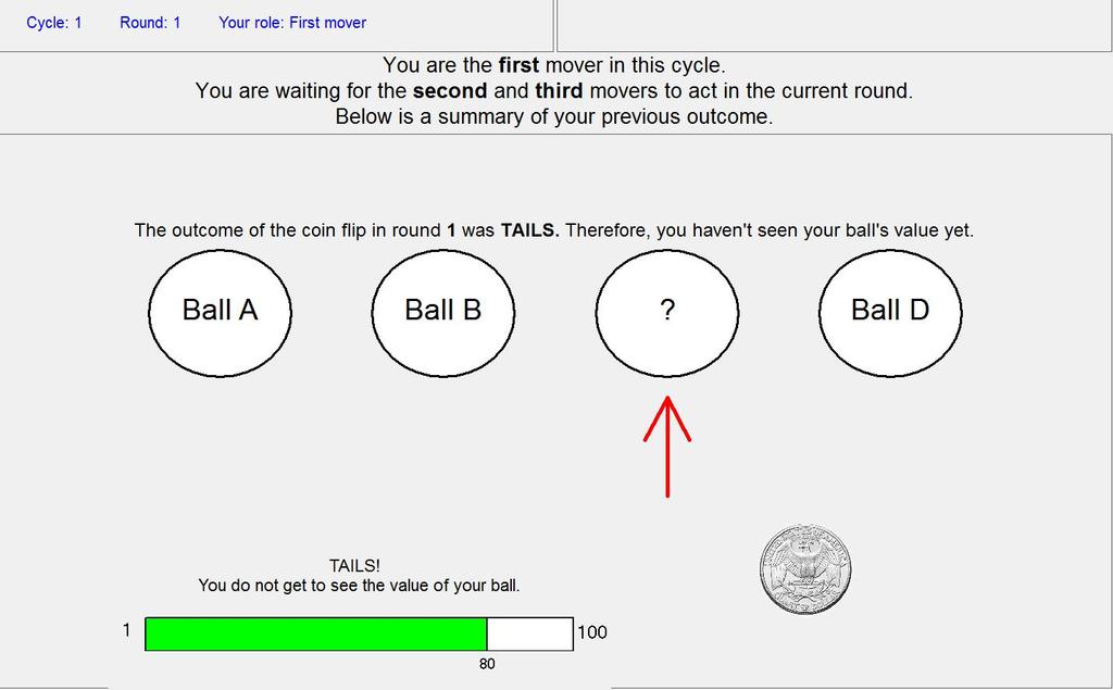
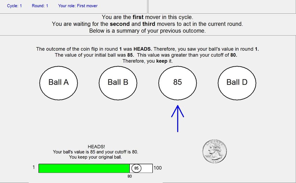
22 APPENDIX C. INSTRUCTIONS C.1. Instructions to Part 1 [Supergames 1-5] 3. C.1.1. No Selection (Control) and S-Explicit 4. Introduction. Thank you for participating in our study. Please turn off mobile phones and other electronic devices. These must remain turned off for the duration of the session. This is an experiment on decision making. The money you earn will depend on both your decisions and chance. The session will be conducted only through your computer terminal; please do not talk to or attempt to communicate with any other participants during the experiment. If you have a question during this instruction phase please raise your hand and one of the experimenters will come to where you are sitting to answer your question in private. During the experiment, you will have the opportunity to earn a considerable amount of money depending on your decisions. At the end of the experiment, you will be paid in private and in cash. On top of what you earn through your decisions during the experiment, you will also receive a $6 participation fee. Outline. Your interactions in this experiment will be divided into Cycles. In each cycle you will be holding one of four balls, called Balls A to D. Each ball has a value between 1 and 100, and your payoff in each cycle will be determined by the value of the ball you are holding at the cycle s end. Initially you will not know any of the four ball s values, and will only know which of the four balls you are holding. Each cycle is divided into three rounds, and in one of these rounds you will see the value of your ball. At the point when you see your ball s value you will be asked to make your only choice for the cycle: either keep the ball you are holding. or instead let go of your current ball and take hold of one of the other three balls. Main Task. In more detail, a cycle proceeds as follows: In each new cycle and for each participant, the computer randomly draws four balls. Each ball s value is chosen in an identical manner: With 50% probability the computer rolls a fair hundred-sided die: so the ball has an equal probability of being any number between 1 and 100. With 25% probability the ball has value 1. 3 Instructions were distributed at the beginning of the experiment and read aloud. 4 Some passages are different depending on treatment, and are indicated by highlighted text and the name of the treatment in brackets. Everything else is the same. 22

23 With 25% probability the ball has value 100. After drawing the values for the four balls, the computer randomly shuffles them into positions A to D. Once in place, the four balls positions are fixed for the entire cycle. So whatever the value on Ball A, this is its value for the entire cycle. Only at the end of each cycle are four new balls drawn for your next cycle. Once the balls are in position, the computer randomly matches you to a ball, so you start out holding one of the balls A to D. There are therefore three leftover balls which are held by the Computer. For example, one possible initial match might be that you hold Ball B. So because Ball B is held in this example, the Computer starts the cycle holding Balls A, C and D. Your outcome each cycle will depend only on the ball you are holding at the end of the cycle. In each cycle you will know which of the four balls you start out holding. You will not know any of the four balls values to start with. Every cycle you will make just one decision. At some random point in the cycle you will be told your ball s value. You will then be asked to make a choice after learning your ball s value: either keep holding your ball or give your ball to the computer, and instead take one of the three balls the computer is holding. The point in the cycle when you see your ball s value is random. Each cycle is divided into three rounds where you are given a chance to see your ball. The round in which you will see your held ball s value and make your choice for the cycle is random: In round one, the computer flips a fair coin. If the coin lands Heads, you will see your ball s value. So you have a 50% chance of seeing your ball s value in the first round. In round two, if you did not see you ball in round one you get another 50% chance of seeing its value: another coin flip. Finally, in round three, if you did not see your ball s value in either round one or round two you will see its value for sure in round three and make your choice. Whenever you do see your held ball s value either in round one, two or three you will make your only decision for the cycle. The two options you have are: (1) Keep hold of your ball until the end of the cycle. (2) Switch balls: Give your ball to the computer to hold, and instead take one of the balls it is currently holding. [S-Explicit] 23

24 If you do choose to switch balls with the computer, the procedure the computer uses to select a ball to give you in exchange varies with the round: In round one, the computer will randomly select one of the three available balls, choosing between each of the three balls it is holding with equal probability. In round two, the computer will randomly select a ball from the two lowest value balls of the three it is holding, choosing each of the two lowestvalue balls with equal probability. So, in round two the computer will never offer you the highest-value ball of the three. In round three, the computer will only offer you the lowest-value ball of the three it is holding. Your cycle payoff is $0.10 multiplied by the number on the ball you are holding at the end of the cycle. So a ball with value 1 at the end of a cycle has a payoff of $0.10, a ball with value 50 has a payoff of $5.00, while a ball with value 100 has a payoff of $ Cycle Summary. (1) Each participant is given four balls A to D, where each ball has a random value between 1 and 100. (2) Each participant is then assigned one of the four balls to hold, with the leftover balls held by the computer. (3) Across three rounds the participants are given the chance to see the value of the balls they are holding. Whenever you see the value of the ball you are holding you must decide whether to keep holding it, or trade it with the computer. In rounds one and two you have a 50% probability of seeing the held ball s values. Any participant that reaches round three without seeing their ball s value will always see its value in round three, and are then given the option to trade it for one of the computer balls. [S-Explicit] The procedure the computer uses to choose the ball it is willing to exchange with you changes across the cycle. In round one it will randomize across all three balls. In round two, it randomizes over the two lowestvalue balls. In round three, it will offer the lowest-value ball with certainty. Experiment Organization. There will be three parts to this experiment. The first part will last for 5 cycles. After this you will get instructions for the second part which will last for another 15 cycles, where the task is very similar. Part 3 will last for a single cycle. 24

25 Following part 3, we will conclude the experiment with a number of survey questions for which there is the chance for further payment. Payment. Monetary payment for Parts 1 and 2 will be made on two randomly chosen cycles, where each of the 20 cycles in the first two parts are equally likely to be selected for payment. You will be given the opportunity for further earnings in Part 3 and the survey at the end of the experiment (which we will explain once the preceding parts end). All participants will receive a $6 participation fee added to total earnings from the other parts of the experiment. C.1.2. Selection, S-Across, S-Within, and S-Peer 5. Introduction. Thank you for participating in our study. Please turn off mobile phones and other electronic devices. These must remain turned off for the duration of the session. This is an experiment on decision making. The money you earn will depend on both your decisions and chance. The session will be conducted only through your computer terminal; please do not talk to or attempt to communicate with any other participants during the experiment. If you have a question during this instruction phase please raise your hand and one of the experimenters will come to where you are sitting to answer your question in private. During the experiment, you will have the opportunity to earn a considerable amount of money depending on your decisions. At the end of the experiment, you will be paid in private and in cash. On top of what you earn through your decisions during the experiment, you will also receive a $6 participation fee. Outline. Your interactions in this experiment will be divided into Cycles. In each cycle you will be in a group of three, with each participant holding one of four balls, called Balls A to D. Each ball has a value between 1 and 100, and your payoff in each cycle will be determined by the value of the ball you are holding at the cycle s end. At the start of each cycle you will see which ball each of the three participants are holding. However, you will NOT know any of the four ball s values. Each cycle is divided into three rounds, and in one of these rounds you will see the value of your ball. At the point when you see your ball s value you will be asked to make your only choice for the cycle: either keep the ball you are holding. 5 Some passages are different depending on treatment, and are indicated by highlighted text and the name of the treatment in brackets. Everything else is the same. 25

26 or instead let go of your current ball and take hold of whichever ball is not being held by another group member. Main Task. In more detail, a cycle proceeds as follows: At the start of each cycle the computer randomly divides all of the participants in the room into groups of three. Each player will randomly be given one of three roles: either First Mover, Second Mover or Third Mover. The groups of three and specific roles assigned are fixed for each cycle. In each new cycle you will be randomly matched into a new group of three. In each new cycle you will be randomly assigned to either be the First, Second or Third Mover. In each new cycle and for each separate group of three, the computer randomly draws four balls. Each ball s value is chosen in an identical manner: With 50% probability the computer rolls a fair hundred-sided die: so the ball has an equal probability of being any number between 1 and 100. With 25% probability the ball has value 1. With 25% probability the ball has value 100. After drawing the values for the four balls, the computer randomly shuffles them into positions A to D. Once in place, the four balls positions are fixed for the entire cycle. So whatever the value on Ball A, this is its value for the entire cycle. Only at the end of each cycle are four new balls drawn for your next cycle and next group of three. Once the balls are in position, the computer randomly gives a different ball to each of the three group members. Each group member therefore starts out holding one of the balls A to D. But because the three group members are each holding one of the four balls there is one leftover ball. This leftover ball is held by the Computer. For example, one possible initial match might be that Ball A is held by the Third Mover; Ball B by the First Mover; and Ball D by the Second Mover. So because Balls A, B and D are all held in this example, the Computer starts the cycle holding the leftover Ball C. [Selection, S-Across, and S-Peer] Your outcome each cycle will depend only on the ball you are holding at the end of the cycle. In each cycle you will know which of the four balls you start out holding You will not know any of the four balls values to start with, nor which balls the other two group members are holding. [S-Within] Your outcome each cycle will depend only on the ball you are holding at the end of the cycle. 26

27 You will not know any of the four ball s values to start with. You will know which ball is being held by each participant, and will also know if a ball was previously held by another participant. Every cycle you will make just one decision. At some random point in the cycle you will be told your ball s value. You will then be asked to make a choice after learning your ball s value: either keep holding your ball or give your ball to the computer, and instead take whichever ball the computer is holding. The point in the cycle when you see your ball s value is random. Each cycle is divided into three rounds where each group member is given a chance to see their ball. Each round is further divided into a sequence of turns, dictated by your role: (1) The first mover gets the first opportunity to see their ball s value. If they see it, they make their one choice for the cycle, if not they must wait until the next round for another opportunity to see their ball s value. (2) After the first mover, the second mover gets an opportunity to see their ball. Again, if they see it, they make their one choice for the cycle, otherwise they must wait until the next round. (3) Finally, after both the first and second mover, the third mover gets an opportunity to see their ball. As before, if they see their ball they make their one choice for the cycle, otherwise they must wait until the next round. The round in which you will see your held ball s value and make your choice for the cycle is random: In round one, the computer flips a fair coin once for each group member. If the coin lands Heads, the group member sees their ball s value. So each group member has a 50% chance of seeing their ball s value in the first round. In round two, any group members who did not see their ball in round one get another 50% chance of seeing its value: another coin flip. Finally, in round three, any group members who did not see their ball in either round one or round two see their ball s value for sure in round three and make their choice. Whenever you do see your held ball s value either in round one, two or three you will make your only decision for the cycle. The two options you have are: (1) Keep hold of your ball until the end of the cycle. (2) Switch balls: Give your ball to the computer to hold, and instead take the ball it is currently holding. The cycle ends after every participant within a group sees the ball s value and makes a decision. [S-Across] 27

28 At the end of the cycle you will get feedback on what happened. You will be told: The balls each group member and the computer started with. Choice 1/2/3: The identity of the group member who was 1st/2nd/3rd to see their ball s value; the round they saw their ball s value; their choice (keep or switch); and which ball the computer was holding after their choice. Your cycle payoff is $0.10 multiplied by the number on the ball you are holding at the end of the cycle. So a ball with value 1 at the end of a cycle has a payoff of $0.10, a ball with value 50 has a payoff of $5.00, while a ball with value 100 has a payoff of $ Cycle Summary. (1) The computer randomly forms the participants in the room into groups of three. (2) Each group is given four balls A to D, where each ball has a random value between 1 and 100. (3) Each of the three participants are given one of the four balls to hold, with the leftover ball held by the computer. (4) Across three rounds the group members move in sequence according to their roles, and each are given the chance to see the value of the ball they are holding. Whenever you see the value of the ball you are holding you must decide whether to keep holding it, or trade it with the computer. In rounds one and two each group member has a 50% probability of seeing their held ball s value. Any group members that reach round three without seeing their ball s value will always see it in round three, and are then given the option to trade it for the current computer ball. Experiment Organization. There will be three parts to this experiment. The first part will last for 5 cycles. After this you will get instructions for the second part which will last for another 15 cycles, where the task is very similar. Part 3 will last for a single cycle. Following part 3, we will conclude the experiment with a number of survey questions for which there is the chance for further payment. Payment. Monetary payment for Parts 1 and 2 will be made on two randomly chosen cycles, where each of the 20 cycles in the first two parts are equally likely to be selected for payment. You will be given the opportunity for further earnings in Part 3 and the survey at the end of the experiment (which we will explain once the preceding parts end). All participants will receive a $6 participation fee added to total earnings from the other parts of the experiment. 28

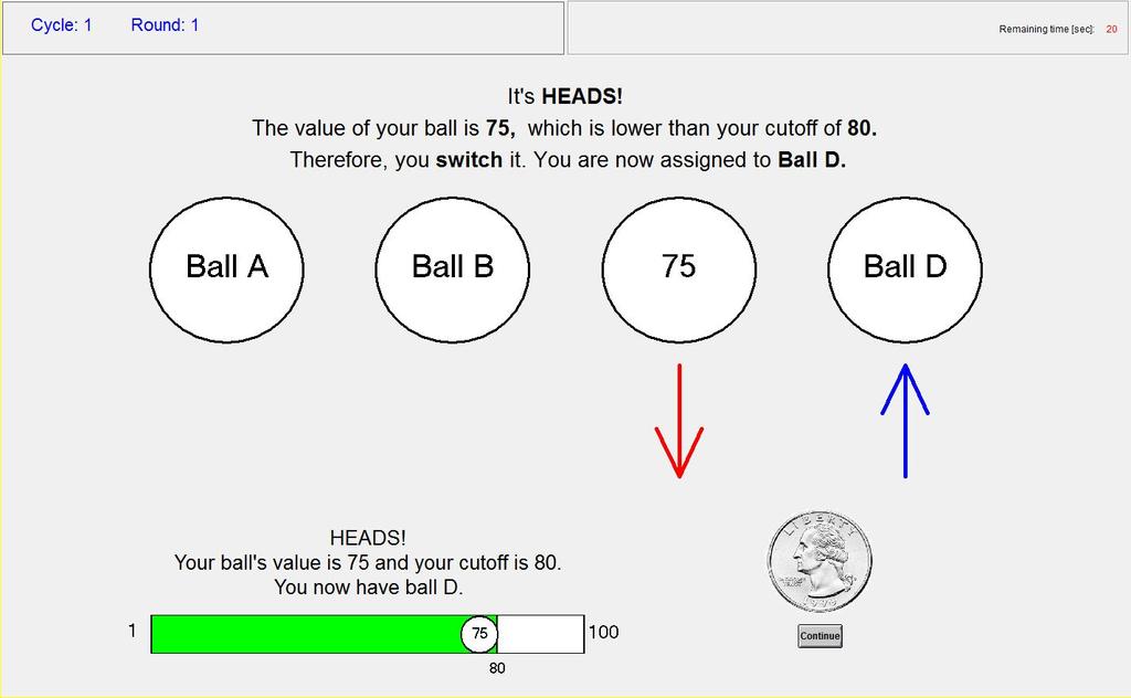
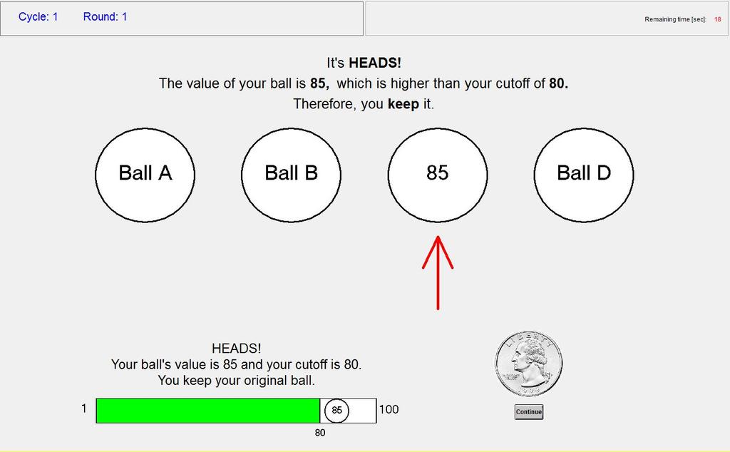
29 C.2. Instructions to Part 2 [Supergames 6-20] 6. We will now pause briefly before continuing on to the second part of the experiment. The task for the next 15 cycles of the experiment is very similar to the last 5. In fact, there is only one difference from part one. So far, if you flipped a head you have been told the value of the ball you are holding prior to deciding whether or not to trade it for the computer s ball. For the remaining cycles you instead will be asked to provide a cutoff rule in case you see your ball. This cutoff is the minimum value you would need to keep the ball you are holding. In every round of a cycle, you will be asked to provide a cutoff for trading your ball should you see its value that round. You will be asked to choose your cutoff value by clicking on the horizontal bar at the bottom of your screens per the projected slide. You can click anywhere on the bar to change your cutoff, and you can always adjust your minimum cutoff by plus or minus one by clicking on the two buttons below the bar. In the projected example I selected a minimum cutoff of 80. After you submit your cutoff the computer will then flip the coin if you are in rounds one or two to determine if you see your ball s value, similar to part one. If the coin flip is tails, nothing happens, and you will have to wait to decide until at least the next round, where you will repeat this procedure and provide another minimum cutoff. If instead the coin flip is Heads, or you are making your decision in round three where you are guaranteed to see your ball, the computer will show you the value of your ball. The computer will automatically keep it or trade your ball according to the minimum cutoff you selected. If your ball s value is LOWER than your selected minimum, you will automatically trade your ball for the computer s ball, which you will keep until the end of the cycle. In the projected example I had selected 80 as my minimum cutoff. In the above example, it shows what would happen if I saw my held ball, and its value was 75. Because this is lower than my selected minimum value of 80, the computer uses my selected cutoff to automatically trade my ball for the computer s ball, rather than keeping it. The next example shows what happens if the coin flip is heads, and your held ball is equal to or greater than your selected minimum cutoff. In this case, because the ball s value is greater than my selected minimum value of 80, the computer uses my selected cutoff to automatically keep my ball until the end of the cycle, rather than trading it. The projected example illustrates what would happen if my held ball had a value of 85. Because 85 is above my selected cutoff of 80, I would keep my ball until the end of the cycle. 6 The experimenter read the instructions aloud after Part 1 had ended. Slides were used to show screenshots and emphasize important points (see section C.3). The text was identical for all treatments, and the accompanying slides differ only for treatment S-Within. 29

30 Because of this procedure, you will maximize your potential earnings by selecting the chosen cutoff value to answer the following question: What is the smallest value X for which I would keep my ball right now, where for any balls lower than X, I would rather trade them for the computer s ball? The computer will now ask you three questions to make sure you understand this cutoff. At the top of your screens the computer will indicate a ball you are holding. Just for these question we will also tell you the ball the computer is holding. For each question we will give you a selected cutoff, and the value of the ball you are holding. Given this information, we would like you to select what happens. You must answer all three questions correctly for the experiment to proceed. 30

31 C.3. Slides for Instructions to Part 2. 31

32 32

33 C.4. Handouts for Part 2 [Supergames 6-20] 7. C.4.1. No Selection (Control) and S-Explicit 8. Part Two. Everything in part two cycles will be the same as part one, with one exception. In every round, you will be asked to provide a cutoff. The cutoff you provide is the minimum value required for you to keep your ball. After you have confirmed your cutoff X between 1 and 100 the computer will determine if you see your ball s value this round: If you see your ball s value this round a choice will be made according to your minimum-value cutoff. If you do not see your ball s value this round, you will provide another minimumvalue cutoff in the next round. In the round where you see your ball, the computer will use your minimum cutoff X as follows: IF your ball s value is equal to or greater than the minimum cutoff X, then you will choose to keep your ball. [No Selection (Control)] OTHERWISE if your ball s value is less than the minimum cutoff X, the computer will choose to trade your ball for one of the computer s balls. [S-Explicit] OTHERWISE if your ball s value is less than the minimum cutoff X, the computer will choose to trade your ball for the one chosen by the computer that round. [Selection, S-Across, S-Within, and S-Peer] OTHERWISE if your ball s value is less than the minimum cutoff X, the computer will choose to trade your ball for the one held by the computer that round. Because of this procedure, you should choose your cutoff value to answer the following question: [No Selection (Control)] What is the smallest value X from 1 to 100 for which I would like to keep my ball right now, rather than give it to the computer in exchange for one of the balls the computer is holding? [S-Explicit] 7 The experimenter distributed the handouts before showing the slides and reading the script. They served as a consultation material for subjects. 8 Some passages are different depending on treatment, and are indicated by highlighted text and the name of the treatment on brackets. Everything else is the same. 33

34 What is the smallest value X from 1 to 100 for which I would like to keep my ball right now, rather than give it to the computer in exchange for its selected ball for this round? [Selection, S-Across, S-Within, and S-Peer] What is the smallest value X from 1 to 100 for which I would like to keep my ball right now, rather than give it to the computer in exchange for the ball the computer is holding? C.5. Instructions to Part Three 9. C.5.1. No Selection, Selection, S-Across, S-Explicit, and S-Within. We will now pause briefly before continuing on to the third part of the experiment. The task for the final cycle of the experiment is very similar to the last 20. However, where we paid two random cycles from the last 20, we will pay you whatever you earn in this last cycle for sure. So for this one cycle you will earn between $0.10 and $10.00 depending on your final ball. In this cycle we will randomly assign you to be either a first, second or third mover, and will tell you your role. Like the preceding rounds, we will ask you for a minimum cutoff value to keep your ball, and the computer will automatically keep or switch your ball depending on your selected cutoff if you see your balls value that round. [No Selection, Selection, S-Explicit, and S-Across] The only difference in part 3 is that we will only tell you which round you saw your ball s value in at the end of the cycle. [S-Within] There are two differences in Part 3. First, we have removed the information on which balls the other participants are holding. All you will know is which ball you are currently holding. Second, we will now only tell you which round you saw your ball s value and how you decided at the very end of this cycle. You will submit cutoffs in rounds 1 to 3, as before. In the round where you see your ball s value, you will use your selected cutoff for that round to make a decision. [No Selection, Selection, S-Across, and S-Within] If your balls value is lower than your minimal cutoff you will exchange your ball with the one the computer is holding at that point. [S-Explicit] If your ball s value is lower than your minimal cutoff you will exchange your ball with the one the computer has selected to exchange for that round. If your balls value is equal to or greater than your minimum cutoff you will keep your ball for the cycle. Because of this procedure, nothing in the structure of the task has changed from Part 2. So you should make your decisions exactly as before. The new 9 The experimenter read the instructions aloud after Part 2 had ended. Slides were used to show screenshots and emphasize important points (see section C.6). 34

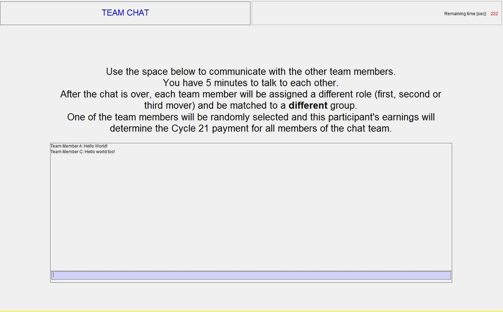
35 procedure allows us to collect information on the cutoffs you would select in all three rounds of the cycle. [No Selection, Selection, S-Across, and S-Explicit] Effectively, the only thing that has changed from part two is the point at which we tell you you have made your choice, and that your payoff from this cycle will always be added to your final cash payoff for the experiment. [S-Within] Recall that, in contrast to the previous cycles, (i) you will now not receive any information about which balls the other two participants and the computer are currently holding in any period, and (ii) you will choose a cutoff in all three rounds. In terms of payment, remember that the outcome from this cycle will always be added to your final cash payoff for the experiment, so that the ball you are holding at the end of this cycle will add between $0.10 and $10.00 to your final payoff, depending on the ball you are holding at the end. Please now make your choices for the final cycle. C.5.2. S-Peer. We will now pause briefly before continuing to Part 3 of the experiment. Part 3 will last for just one cycle, and this cycle will be paid with certainty. So you will earn between $0.10 and $10.00 for Part 3. The task for the final cycle of the experiment is very similar to the last 20. Like the preceding rounds, we will randomly assign you to be either the first, second, or third mover, and we will ask you for a minimum cutoff to keep your ball. The computer will then automatically keep or switch your ball depending on your selected cutoff and the value of your ball. The first difference in Part 3 is that we will only tell you which round you saw your ball s value at the very end of the cycle. That is, you will submit cutoffs for rounds 1 to 3, as before. In the round where you see your ball s value, we will use your selected cutoff for that round to make a decision. (1) If your ball s value is lower than your minimum cutoff, you will exchange your ball with the one the computer is holding at that time. (2) If your ball s value is equal to or greater than your minimal cutoff, you will keep your ball for the cycle. Because of this procedure, nothing in the structure of the task has changed from Part 2. The new procedure is chosen to allow us to collect information on the cutoffs you would select in all three rounds of the cycle. The second difference from the first 20 cycles is the determination of payment for Part 3. Before you go on to Part 3, you will be matched into a team of three participants. This team will be given the chance to communicate with each other, prior to making their choices in Part 3. After the chat is completed, each team member will be assigned to a different role (first, second, or third mover), and each of the three team members will be 35

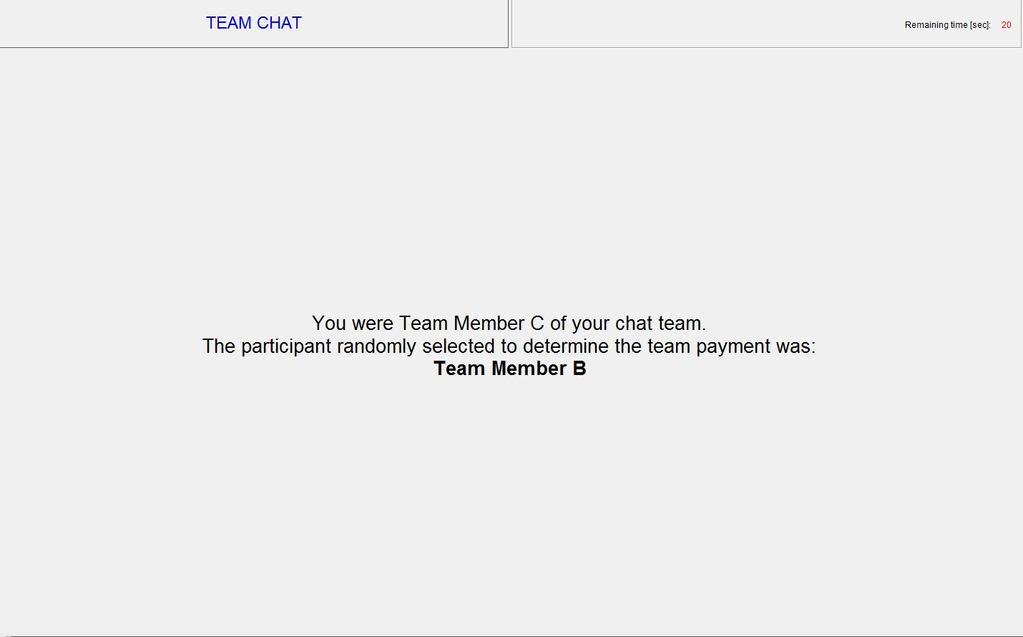
36 assigned to different groups with participants from other teams. Each team-member will then make their choices in the final cycle. Payment for Part 3 for your entire team (the participants you will chat with) will be determined by the actions of one randomly selected team member. The chat window allows you to discuss your possible cutoff choices with your other team members before the cycle begins. This is what the chat screen looks like. You will have 5 minutes to discuss with your team members what to do in cycle 21. You may not use the chat to discuss details about your previous earnings, nor are you to provide any details that may help other participants in this room identify you. This is important to the validity of the study and will not be tolerated. However, you are encouraged to use the chat window to discuss the choices in the upcoming cycle. In particular, because of our modification to the cutoff procedure, all three team members will make three cutoff choices: the cutoff decision for each round one, two and three. Whatever advice you can provide your matched team-members that leads them to a better outcome in Part 3 will also benefit you, as there is a two-in-three chance that one of the other team member s choices will define your earnings for this part. Similarly, the advice of others can also help you, as there is a one-in-three probability that your choices will define both your earnings for Part 3 as well as the earnings of the other two teammembers. After the Part 3 cycle is completed, one of the three team members will be randomly selected and that participant s final held ball will determine the payment for all three members of the team. We will then show you the outcome of the chosen cycle, as in the projected slide. We will pay you for whatever you earn in this last cycle for sure. So for Part 3 you will earn $0.10 times the value of the ball the selected team member is holding at the end of the cycle. 36

37 C.6. Slides for Instructions to Part 3. C.6.1. No Selection, Selection, S-Across, S-Explicit, and S-Within. Part Three will consist of a single cycle Whatever you earn in this cycle will be added to the two random cycles selected from Parts 1 and 2 So you have the chance to earn between $0.10 and $10.00 for this cycle depending on your final ball You will be told whether you are the First, Second or Third mover We will ask you for your minimal cutoff in each new round as before If your coin flip is heads, you will choose an action according to your cutoff as before The only difference is that we will not tell you when and if you have made a choice until the end of the cycle 37

38 You will submit cutoffs in rounds 1 to 3, as before In the round where you see your ball s value, you will use your selected cutoff to make a decision If your balls value is lower than your minimal cutoff you will exchange your ball with the one the computer is holding If your balls value is equal to or greater than your minimal cutoff you will keep your ball Because of this procedure, nothing in the structure of the task has changed The new procedure allows us to collect information on the cutoff you would select in all three rounds All that has changed from part two is the time at which we inform you on your choice for the cycle 38

39 C.6.2. S-Peer. Part Three will consist of a single cycle Whatever you earn in this cycle will be added to the two random cycles selected from Parts 1 and 2 So you will earn between $0.10 and $10.00 for this cycle We will ask you for your minimal cutoff in each new round as before If your coin flip is heads, you will choose an action according to your cutoff as before The only difference is that we will not tell you when and if you have made a choice until the end of the cycle You will submit cutoffs in rounds 1 to 3, as before In the round where you see your ball s value, you will use your selected cutoff to make a decision If your balls value is lower than your minimal cutoff you will exchange your ball with the one the computer is holding If your balls value is equal to or greater than your minimal cutoff you will keep your ball Because of this procedure, nothing in the structure of the task has changed. The new procedure allows us to collect information on the cutoff you would select in all three rounds All that has changed from part two is the time at which we inform you on your choice for the cycle 39

40 40

41 41

42 42

43 C.7. Instructions for Part 4. Finally we will conduct a number of survey questions for which there will be the chance of an additional payment. Part four consists of three sets of questions, which will have a series of possible prizes. One participant in the room will be randomly selected for payment on these additional questions. The first question is a decision making task. You will be presented with three balls. One of these balls is worth $10, while the other two are worth $0. The computer has shuffled the three balls, and fixed their locations. (1) We will ask you to choose one of the the three balls. (2) After you have chosen a ball, we will reveal one zero dollar ball from the two balls that you did not choose. (3) We will then make you an offer: Would you like the ball you initially chose plus $5? Or would you instead like to switch to the remaining ball plus X times $0.10? X will vary between 1 and 100. We would like you to tell us the minimum value of X for which you would like to swap. If you swap you get the value of the remaining unchosen ball (either 0$ or $10) plus $0.10 times X (so between $0.10 and $10) If you keep your ball, you get its value (either 0$ or $10) plus $5. Please make your choices for this task now. [Wait while subjects complete task] The next task will ask you to answer three numerical questions within a 15 second time-limit. Whoever is selected for payment in part 4 will receive $1 per correct answer. [Wait while subjects complete task] Finally, we would like you to make a series of choices between lotteries. In each choice you will be asked to pick either Lottery A or Lottery B, where each offers a probability over two monetary prizes. One of your four choices from these lotteries will be selected for payment, and the outcome added to your total earnings if you are selected for payment in part four. 43

44 APPENDIX D. SCREENSHOTS 44

45 45

46 46