SDMR Finance (2) Olivier Brandouy. University of Paris 1, Panthéon-Sorbonne, IAE (Sorbonne Graduate Business School)

Transcription

1 SDMR Finance (2) Olivier Brandouy University of Paris 1, Panthéon-Sorbonne, IAE (Sorbonne Graduate Business School)

2 Outline 1 Formal Approach to QAM : concepts and notations 2 3

3 Portfolio risk and return

4 Portfolio basics (1) Asset Universe (a list of selected financial assets that can be traded by the fund manager): i financial assets, i [1, n], denoted ℵ = [a 1, a 2,..., a n ]. Portfolios are combinations of assets over ℵ. A given portfolio is simply defined as a vector of weights W k = w 1, w 2,..., w i, k [1, + ] such as k, n i=1 w i = 1. One can define an arbitrarily large number of portfolios over ℵ (for example with Monte Carlo simulations). Remark (Short selling) Notice that some weights may be negative (which means short selling ). This must be taken into account when interpreting risk-return relations (see below). Going short may be done borrowing assets to someone and selling them immediately. They will be repurchased later to return to the lender (investors who are structurally long, REPO activity).

5 Portfolio moments (1) E[r p ] = n i=1 w ie[r i ] Portfolio variance is usually considered as measure of Portfolio risk. Notice this measure only focuses on the second moment of portfolio returns distribution. Agents May also have preferences on higher moments. Portfolio risk is more complicated than the mere linear combination of asset risks. This is linked o the fact that E[R i ] are not independent random variables. For two assets i, j ℵ we can define a Pearson product-moment correlation coefficient ρ i,j = Notice that cov i,j = ρ i,j σ i σ j cov(i, j) σ i σ j = E((i µ i)(j µ j )) σ i σ j

6 Portfolio moments (2) Definition n n n n σp 2 = w i w j cov i,j = w i w j ρ i,j σ i σ j i=1 j=1 i=1 j=1 The n assets ℵ exhibit a certain level of association which delivers a variance-covariance matrix : cov 1,1 cov 1,2... cov 1,n cov 2,1 cov 2,2... cov 2,n A = cov n,1 cov n,2... cov n,n

7 Matrix algebra approach cov 1,1 cov 1,2... cov 1,n cov 2,1 cov 2,2... cov 2,n A = cov n,1 cov n,2... cov n,n W = w 1 w 2. w n Definition (waw!) σ 2 p = t W.A.W

8 Portfolio moments (3) Remark (Linear combination of Standard Deviations) For two assets i, j and when ρ ij = 1 : σ 2 p = w 2 i σ 2 i + w 2 j σ 2 j + 2w i w j cov i,j = (w i σ i + w j σ j ) 2 Remark (Case on absence of autocorrelation among assets) Even if i jρ ij = 0 portfolio variance weighted sum of individual asset variances but the sum of these variances times the square of individual weights.

9 A basic 2-assets illustration See example 2assetsBasics.odt Compute 1 expected returns 2 variance-covariance matrix (and correlation XY) Table: Two Assets, Joint distribution Possible return for X Marginal dist. For Y Possible return Y Marginal dist. For X

10 Expected Returns & Joint Probability distribution (1) 1 Expected returns E(R i ) i R i.p i 2 Variance V (R i ) i (R i R ) 2.p i 3 Covariance cov i,j i (R i R i )(R j R j )2.p i,j 4 Correlation ρ i,j cov i,j /(σ i σ j ) Table: Moments - Co-moments X Y E(R) Var StD cov ρ

11 Portfolios and Risks, a first look One can generate as many portfolios as desired (Monte Carlo procedure) 1 Generate randomly w X and w Y such as w X + w Y = 1 2 Compute portfolio risks using equation previously exposed Remark (Minimum Variance Portfolio) Starting from w X + w Y = 1 and searching for a null derivative : σ 2 p = w 2 X σ 2 X + (1 w X ) 2 σ 2 Y + 2w X (1 w X )cov XY dσ 2 p dw X = 2w X σ 2 X 2(1 w X )σ 2 Y + 2(1 2w X )cov XY = 0 wx σy 2 = cov XY σx 2 + σ2 Y 2cov XY

12 Effect of Correlation on Portfolio Risks See 2assetsBasics.ods Without short selling (all weights are > 0) When ρ > 0 X reinforces Y (and reciprocally) in common effects / portfolio risks and returns. When ρ < 0 X weakens Y (and reciprocally) in common effects / portfolio risks and returns. The greater ρ (in absolute value), the stronger these effects. With short selling (all opposite) rho = 0.5 rho = 0.1 rho = -0.5 X no shorting Y shorting

13 DIY! Formal Approach to QAM : concepts and notations Consider 2 assets X and Y with the following statistics : r X = 0.14, r Y = 0.2 σ X = 0.15, σ Y = 0.25 ρ = 0.2 Could you compute : The minimum risk portfolio? The optimal portfolio delivering a return of 17%? Give the associated level of risk for this asset?

14 Portfolio Selection, the Markowitz approach

15 Markowitz General Framework Definition Seminal paper: Harry Markowitz (1952), Portfolio Selection, The Journal of Finance, 7(1), Among possible portfolios, a limited set is said to be efficient in the sense that, for any given target return, it is not possible to obtain from any combination of assets in the underlying universe a lower level of risk. For Markowitz, the investor is solely interested in the first two moments: The E- V rule states that the investor would (or should) want to select one of those portfolios which give rise to the (E, V) combinations indicated as efficient in the figure; i.e., those with minimum V for given E or more and maximum E for given V or less.

16 Implications (1) Utility functions for the investor can be described as favoring odd moments (m 1 ) and discounting even moments (m 2 ). Markowitz Utility Functions : ( U/ E[r p ]) > 0 and ( U/ σ 2 [r p ]) < 0 E[U(r p )] = E[r p ] γe[r 2 p ] = r p + γr p 2 γσ 2 r p The greater the risk, the greater the expected return (non-linear relation) The higher in the Figure the indifference curve, the more appreciated the risk-return combination. E[rp] U1 U2 U3 E*

17 Implications (2) Definition Investors should invest in the portfolio at the tangency point between their Utility Function and the Optimal Set. U1 E[rp] U2 E* Portefeuille optimal V* V[rp] This leads i) to characterize the investor Utility function (see B. Munier) and ii) to a non-linear programming problem where one seeks to minimize the portfolio variance, under a series of constraints and for a given target return.

18 Mathematical formulation of the problem (no shorting) 1 min st. = n i=1 j=1 n w i w j σ ij n i=1 w ir i = r p n i=1 w i = 1 i, w i 0 This program is equivalent to the minimization of the following Lagrangian function: L = n i=1 j=1 n ( n w i w j σ ij + λ 1 w i r i rp ) ( n + λ2 w i 1 ) i=1 i=1

19 Mathematical formulation of the problem (no shorting) 2 We therefore obtain n + 2 linear equations: L w 1 = 2w 1 σ 1,1 + 2w 2 σ 1, w n σ 1,n + λ 1 r 1 + λ 2 = 0... L w n = 2w 1 σ n,1 + 2w 2 σ n, w n σ n,n + λ 1 r n + λ 2 = 0 L λ 1 = w 1 r 1 + w 2 r w n r n r p = 0 L λ 2 = w 1 + w w n 1 = 0

20 Mathematical formulation of the problem (no shorting) 3 This system is usually presented under its matrix form A.W = T, with : A = 2σ 1,1 2σ 1,2... 2σ 1,n r σ n,1 2σ n,2... 2σ n,n r n 1 W = r 1 r 2... r n w 1. w n λ 1 λ 2 T = 0. 0 r p 1 Computing the solution leads to the inversion of A such as : (A 1 A)W = A 1 T W = A 1 T

21 Mathematical formulation of the problem (no shorting) 4 In a previous example, we obtained : Table: Moments - Comoments X Y ER VARIANCE SD Covariance optimal for a target rate of return = 3%? A = 2(0.2638) 2( ) ( ) 2(0.0837) W = w 1 w 2 λ 1 λ 2 T =

22 Example with 2 assets (cont.) Computing the solution leads to the inversion of A (see 2assetsBasics.ods): A 1 = This delivers W X = 29% and W Y = 71% One can also use the solver extension system to obtain this result (see spreadsheet) This kind of computation is useful and extremely frequent in AM.

23 A (slightly) more tricky problem In the 2 asset Universe, any portfolio is optimal in the Markowitz sense provided W 1 + W 2 = 1. This is no longer the case when more than 2 assets are considered. BNP, VALEO & ZODIAC in [9/12/ /04/05] (roughly 5 months, threestocks.csv).

24 Individual Assets and Portfolio Moments 1 Compute individual moments and co-moments 2 Compute Portfolio moments with the following assumprion w = { 1 3, 1 3, 1 3 } BNP VALEO ZODIAC Portfolio Mean Variance Standard Deviation Product-moment Correlations BNP VALEO ZODIAC BNP VALEO ZODIAC

25 Monte Carlo Portfolios and optimal set Using the following spreadsheet : portfoliooptim.ods: 1 Generate Monte Carlo Portfolios 2 Characterize the efficient set 3 Identify the minimum risk portfolio 4 Identify the equally weighted portfolio

26 3 Assets Graphical Representation

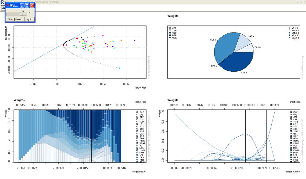
27 An illustration in R

28 Mini-case 1 Download 3 assets from and the CAC 40 index from [13/08/ /12/2004] EADS (EAD.PA) ALCATEL-LUCENT (ALU.PA) LVMH (MC.PA) CAC 40 (ˆFCHI) 2 Compute moments, co-moments 3 Minimum portfolio risk? Composition of this portfolio (without shorting) 4 Composition of the optimal portfolio for the average rate of return (without shorting) 5 Assuming you hold the previous portfolio and that you manage euros, how many stocks would you hold for in each of your portfolio lines? (use the last price you get for your computations.) 6 What do you think of the equally weighted portfolio? Is it Optimal?

29 The limits of diversification VP Number of assets in portfolio (EWP)

30

31 Target of the CAPM 1 Asset Pricing : how do asset prices emerge? 2 Notion of Equilibrium Partial Equilibrium : Portfolio Theory deals with any investor s individual choice General Equilibrium : CAPM tackles the question of equilibrium emergence (S/D) over ALL investors

32 More on equilibrium 1 A coherent Markowitz-Tobin framework No friction in the market (no tax, possibility of short selling) Possibility to lend/borrow at the same r f arbitrarily important amounts of money. r f derives from the confrontation of aggregate positions lenders / borrowers. Investors homogeneous expectations regarding all expected returns : the CML holds for anyone. tangency portfolio is the Market Portfolio. 2 Market clears such as Supply = Demand. In adjusting prices, investors create the conditions to obtain the equilibrium E(r i ) (here-after expected returns will be noted r) 3 Market Portfolio is such as n i.p i w M = n i=1 n i.p i

33 Market / Tangency portfolio : Illustration (1) Consider an economy in which only 3 risky assets A, B, C and one riskless asset r f are traded and where only 3 investors 1, 2, 3 trade these assets. Their total wealth is 500, 1000, 1500 Suppose that the tangency portfolio w T = (w A, w B, w C ) = (0.25, 0.50, 0.25). The decomposition of each investor s holdings is as follows: Investor Riskless A B C Total

34 Market / Tangency portfolio : Illustration (2) Proposition : w T = w M In equilibrium, the total holding of each asset must equal its market value: Market capitalization of A = 750 Market capitalization of B = 1500 Market capitalization of C = 750 Total market capitalization = = The market portfolio is the tangent portfolio: w M = , , = (0.25, 0.50, 0.25) = w T (1)

35 Link between Risk and Price As we will show later, CAPM states that : r i = r f +Market Price of Risk Quantity of risk i CAPM must therefore answer two questions : 1 What is the Market reward for Risk? 2 What is the quantity of Risk included in i?

36 Illustration Let s consider 2 assets X with r X = 0.14 and σ X = 0.2 and Y with r Y = 0.10 and σ Y = What is the market reward for Risk? 2 What is the quantity of risk included in i? Any problem here? X seems less risky than Y but receives a higher return... Is there something wrong?

37 Illustration Let s consider 2 assets X with r X = 0.14 and σ X = 0.2 and Y with r Y = 0.10 and σ Y = What is the market reward for Risk? 2 What is the quantity of risk included in i? Any problem here? X seems less risky than Y but receives a higher return... Is there something wrong?

38 Answers of the CAPM 1 At the equilibrium, the market pays the same reward for Risk whatever the tradable assets. 2 TOTAL risk of assets is not rewarded (σ), only part of it will: Total Risk = Systematic (cannot be eliminated by diversification) Risk + Specific Risk (can be)

39 Formally (the Security Market Line): Market Reward of Risk : [ (r) M r f ] Quantity of Risk Rewarded by the market for asset i : β i = cov i,m σ 2 M In equilibrium, for all assets : r i = r f + cov i,m σm 2.[ r M r f ] = r f + β i.[ r M r f ] E[rp] E(R M ) Market Portfolio [E(rM)-rf] (0,rf) 1 β i

40 Understanding the CAPM (1) 1 There are k = 1, 2,..., K investors. 2 Investor k has wealth W k and invests in two funds: W k rf in riskless asset W k W k rf in the tangent portfolio w T.

41 Understanding the CAPM (2) : Market equilibrium - demand equals supply 1 Money Market Equilibrium : K k=1 W k rf = 0 2 Stock Market Equilibrium : K k=1 (W K W k rf )w T = MCap M w M Since the net amount invested in the risk-free asset is zero, all wealth is invested in stocks: K W K = MCap M (2) k=1 Thus, the total wealth of investors equals the total value of stocks: w T = w M The tangent portfolio is the market portfolio!

42 CAPM : Consequences 1 The market portfolio is the tangent portfolio. 2 Combining the risk-free asset and the market portfolio gives the portfolio frontier. 3 The risk of an individual asset is characterized by its covariability with the market portfolio. 4 The part of the risk that is correlated with the market portfolio, the systematic risk, cannot be diversified away. Bearing systematic risk needs to be rewarded. 5 The part of an asset s risk that is not correlated with the market portfolio, the non-systematic risk, can be diversified away by holding a frontier portfolio. Bearing nonsystematic risk need not be rewarded. 6 For any asset i: r i r f = β i ( r M r f ), with β i = σ i σ 2 M (3)

43 Examples Suppose that CAPM holds. The expected market return is 14% and the risk free rate is 5%. What should be the expected return on a stock with β = 0? Answer: Same as the risk-free rate, 5% The stock may have significant uncertainty in its return. This uncertainty is uncorrelated with the market return What should be the expected return on a stock with β = 1? Answer: The same as the market return, 14%.

44 Examples Suppose that CAPM holds. The expected market return is 14% and the risk free rate is 5%. What should be the expected return on a stock with β = 0? Answer: Same as the risk-free rate, 5% The stock may have significant uncertainty in its return. This uncertainty is uncorrelated with the market return What should be the expected return on a stock with β = 1? Answer: The same as the market return, 14%.

45 Examples Suppose that CAPM holds. The expected market return is 14% and the risk free rate is 5%. What should be the expected return on a stock with β = 0? Answer: Same as the risk-free rate, 5% The stock may have significant uncertainty in its return. This uncertainty is uncorrelated with the market return What should be the expected return on a stock with β = 1? Answer: The same as the market return, 14%.

46 Examples (Cont.) What should be the expected return on a portfolio made up of 50% in the risk free rate and 50% market portfolio? Answer: the expected return should be r = (0.5)(0.05) + (0.5)(0.14) = 9.5% What should be expected return on stock with β = -0.6? Answer: The expected return should be How can this be? r = ( 0.6)( ) = 0.4%.

47 Examples (Cont.) What should be the expected return on a portfolio made up of 50% in the risk free rate and 50% market portfolio? Answer: the expected return should be r = (0.5)(0.05) + (0.5)(0.14) = 9.5% What should be expected return on stock with β = -0.6? Answer: The expected return should be How can this be? r = ( 0.6)( ) = 0.4%.

48 Examples (Cont.) What should be the expected return on a portfolio made up of 50% in the risk free rate and 50% market portfolio? Answer: the expected return should be r = (0.5)(0.05) + (0.5)(0.14) = 9.5% What should be expected return on stock with β = -0.6? Answer: The expected return should be How can this be? r = ( 0.6)( ) = 0.4%.

49 A (formal) derivation of the CAPM We start from an idealized situation in which an investor holds w 1 in Asset 1 and w 2 = 1 w 1 in the Market Portfolio. We know that: r p = w 1 r 1 + (1 w 1 ) r M σ p = (w1 2σ 1 + (1 w 1 ) 2 σ M + 2w 1 (1 w 1 )cov 1,M ) Notice that i is part of the Market Portfolio. Thus w 1 is an excess demand for asset i that should not be present in any investor portfolio beyond w1 MP. 1 This is incoherent with market equilibrium conditions along which S = D. 2 w 1 MUST be 0

50 Effect of Market adjustment (1) Under the assumption that market equilibrium will re-appear after some adjustments, the impact on r p and σ p : r p w 1 = r 1 r M σ p = 1 ( (w 2 w σ 1 ) + (1 w 1 ) 2 ) 1 2 σ M ( 2w 1 σ1(1 2 w 1 ) 2σM 2 ) + 2cov 1,M 4w 1 cov 1,M (4) σ p w 1 = cov 1,Mσ 2 M σ M

51 Effect of Market adjustment (2) Therefore, the slope of the risk-return trade-off for the Market Portfolio is : r p / w 1 σ M = ( r 1 r M ) σ p / w 1 cov 1,M σ1 2 On the other hand, the slope of the risk-return delivered by the CML is : r M r f σ M Thus : σ M r 1 r M cov 1,M σ1 2 = r M r f σ M

52 Effect of Market adjustment (3) This latter equation can be re-arranged so to obtain : Definition () r 1 = r f + cov 1,M σ 2 M ( r M r f ) r 1 = r f + β 1 ( r M r f )

53 Consequences of the CAPM In equilibrium Each asset is priced so that its risk-adjusted required rate of return is exactly on the SML. β i quantifies the systematic risk of any asset i, that is, the covariation of the asset with the entire economy. One cannot diversify this risk. The higher β i, the higher the expected rate of return E(r i ) Part of the total risk actually can be diversified (bad or good events supported by the firm)

54 Distinguishing Systematic and Non-systematic Risks When we estimate the CAPM, we can decompose an assets return into three pieces r i r f = α i + β i ( r M r f ) + ɛ i with: 1 E(ɛ i ) = 0 2 cov( r M, ɛ i ) = 0 Thus, the 3 pieces are 1 β 2 σ = StD(ɛ i ) 3 α

55 Distinguishing Systematic and Non-systematic Risks (2) β measures an assets systematic risk. Assets with higher betas are more sensitive to the market. σ measures its non-systematic risk. Non-systematic risk is uncorrelated with systematic risk.

56 Distinguishing Systematic and Non-systematic Risks (3) ( r i r f ) = β i ( r M r f ) }{{} + ɛ }{{} i systematic component non-systematic component Var( r i r f ) = σ 2 ( r i ) = βi 2 σ 2 ( r M ) + }{{} σ 2 ɛ }{{} i systematic risk non-systematic risk

57 Risk decomposition : example Two assets with the same total risk can have very different systematic risks. Suppose that σ M = 20% Stock Business Market beta Residual variance 1 Steel Software For the first asset, we get : σ 2 1 = β 2 1σ 2 M + σ 2 ɛ 1 For the second asset : 0.19 = (1.5) 2 (0.2) σ 2 2 = β 2 2σ 2 M + σ 2 ɛ = (1.5) 2 (0.2) However, asset 1 exhibits much more systematic risk than asset 2!

58 A short case Consider an asset with annual volatility σ of 40% market beta of 1.2. Suppose that the annual volatility of the market is 25%. What percentage of the total volatility of the asset is attributable to non-systematic risk? (0.4) 2 = (1.2) 2 (0.25) 2 + Var(ɛ) Var(ɛ = 0.07) σ ɛ =

59 A short case Consider an asset with annual volatility σ of 40% market beta of 1.2. Suppose that the annual volatility of the market is 25%. What percentage of the total volatility of the asset is attributable to non-systematic risk? (0.4) 2 = (1.2) 2 (0.25) 2 + Var(ɛ) Var(ɛ = 0.07) σ ɛ =

60 The (special) case of α According to CAPM, α should be zero for all assets. α measures an assets return in access of its risk-adjusted award according to CAPM. What to do with an asset of positive α? Check estimation error. Past value of may not predict its future value. Positive may be compensating for other risks.

61 Three important relations deriving from the model 1 The beta of any given portfolio is : β P = i w i β i 2 The total variance of any asset i can therefore be decomposed in two components: σi 2 = βi 2 σm 2 + σɛ 2 i where βi 2σ2 M is the firm s systematic risk and σ2 ɛ i is the specific risk. 3 In terms of proportion, one can also compute the following: 1 = β2 i σ2 M σ 2 i + σ2 ɛ i σ 2 i