3. Capital asset pricing model and factor models

Transcription

1 3. Capital asset pricing model and factor models (3.1) Capital asset pricing model and beta values (3.2) Interpretation and uses of the capital asset pricing model (3.3) Factor models (3.4) Performance indexes 1

2 3.1 Capital asset pricing model and beta values Capital market line (CML) The CML is the tangent line drawn from the risk free point to the feasible region for risky assets. This line shows the relation between r P and σ P for efficient portfolios (risky assets plus the risk free asset). The tangency point M represents the market portfolio, so named since all rational investors (minimum variance criterion) should hold their risky assets in the same proportions as their weights in the market portfolio. If every investor is a mean-variance investor and all have homogeneous expectations on means and variances, then everyone buys the same portfolio. Prices adjust to drive the market to efficiency. 2

3 Based on the risk level that an investor can take, she will combine the market portfolio of risky assets with the risk free asset. 3

4 Equation of the CML: r = r f + r M r f σ M σ, where r and σ are the mean and standard deviation of the rate of return of an efficient portfolio. Slope of the CML = r M r f σ M = price of risk of an efficient portfolio. This indicates how much the expected rate of return must increase when the standard deviation increases by one unit. 4

5 Example Consider an oil drilling venture; current share price of the venture = $875, expected to yield $1,000 in one year. The standard deviation of return, σ = 40%; and r f = 10%. Also, r M = 17% and σ M = 12% for the market portfolio. Question How does this venture compare with the investment on efficient portfolios on the CML? Given this level of σ, the expected rate of return predicted by the CML is r = = 33% The actual expected rate of return = 1,000 1 = 14%, which is well 875 below 33%. This venture does not constitute an efficient portfolio. It bears certain type of risk that does not contribute to the expected rate of return. 5

6 Sharpe ratio One index that is commonly used in performance measure is the Sharpe ratio, defined as r i r f σ i = excess return above riskfree rate. standard deviation We expect Sharpe ratio slope of CML. Closer the Sharpe ratio to the slope of CML, the better the performance of the fund in terms of return against risk. In previous example, Slope of CML = Sharpe ratio of venture = 17% 10% 12% 14% 10% 40% = 7 12 = = 0.1 < Slope of CML. 6

7 Capital Asset Pricing Model (CAPM) Let M be the market portfolio M, then the expected return r i of any asset i satisfies where r i r f = β i (r M r f ) β i = σ im σm 2. Here, σ im is the correlation between the return of risky asset i and the return of the market portfolio M. Remark If we write σ im = ρ im σ i σ M, then r i r f r M r f = ρ im. σ i σ M The Sharpe ratio of asset i is given by the product of ρ im and the slope of CML. 7

8 Assumptions underlying the standard CAPM 1. No transaction costs. 2. Assets are infinitely divisible. 3. Absence of personal income tax. 4. An individual cannot affect the price of a stock by his buying or selling action. 5. Investors are expected to make decisions solely in terms of expected values and standard deviations of the returns on their portfolios. 8

9 6. Unlimited short sales are allowed. 7. Unlimited lending and borrowing at the riskless rate. 8. Investors are assumed to be concerned with the mean and variance of returns, and all investors are assumed to define the relevant period in exactly the same manner. 9. All investors are assumed to have identical expectations with respect to the necessary inputs to the portfolio decision. Both (8) and (9) are called homogeneity of expectations. 9

10 Proof Consider the portfolio with α portion invested in asset i and 1 α portion invested in the market portfolio M. The expected rate of return of this portfolio is and its variance is r α = αr i + (1 α)r M σ 2 α = α 2 σ 2 i + 2α(1 α)σ im + (1 α) 2 σ 2 M. As α varies, (σ α, r α ) traces out a curve in the σ r diagram. The market portfolio M corresponds to α = 0. The curve cannot cross the CML, otherwise this would violate the property that the CML is an efficient boundary of the feasible region. Hence, as α passes through zero, the curve traced out by (σ α, r α ) must be tangent to the CML at M. 10

11 Tangency condition Slope of the curve at M = slope of CML. 11

12 First, we obtain dr α dα = r i r M and so that dσ α dα dσ α dα = ασ2 i + (1 2α)σ im + (α 1)σ 2 M σ α = σ im σm 2. α=0 σ M Next, we apply the relation dr α dσ α = dr α dα dσ α dα to obtain dr α = (r i r M )σ M dσ α α=0 σ im σm 2. However, dr α should be equal to the slope of CML, that is, dσ α α=0 (r i r M )σ M σ im σ 2 M = r M r f σ M. 12

13 Solving for r i, we obtain Now, β i = r i r f r M r f r i = r f + σ im σm 2 (r M r f ) = r f + β i (r M r f ). }{{} β i = expected excess return of asset i over r f expected excess return of market portfolio over r f. Predictability of equilibrium return The CAPM implies that in equilibrium the expected excess return on any single risky asset is proportional to the expected excess return on the market portfolio. The constant of proportionality is β i. 13

14 Alternative proof of CAPM Consider σ im = cov(r i, r M ) = e T i Ωw M, where e i = (0 1 0) = i th co-ordinate vector. Recall w M = Ω 1 (µ r1) b ar so that σ im = (µ r1) i b ar = r i r, provided b ar 0. (1) b ar Also, we recall µ M = c br b ar and σ2 M = c 2rb + r2 a (b ar) 2 so that µ M r = c br b ar r = c 2rb + r2 a (b ar) 2 = (b ar)σ 2 M. (2) Eliminating b ar from eqs. (1) and (2), we obtain r i r = σ im σ 2 M (µ M r). 14

15 What is the interpretation of σ im σ M, where σ im = cov(r i, r M )? Consider σ 2 M = w T M Ωw M, we differentiate with respect to w i and obtain so that 2σ M dσ M dw M i dσ M dw M i = σ im σ M = 2e T i Ωw M = 2σ im or dσ M σ M = β i dw M i. This is a measure of how the change in weight of one asset affecting the relative risk of the market portfolio. 15

16 Beta of a portfolio Consider a portfolio containing n assets with weights w 1, w 2,, w n. Since r P = n i=1 w i r i, we have cov(r P, r M ) = n i=1 w i cov(r i, r M ) so that β P = cov(r P, r M ) σ 2 M = ni=1 w i cov(r i, r M ) σ 2 M = n i=1 w i β i. 16

17 Some special cases of beta values 1. When β i = 0, r i = r f. A risky asset (with σ i > 0) that is uncorrelated with the market portfolio will have an expected rate of return equal to the risk free rate. There is no expected excess return over r f even the investor bears some risk in holding a risky asset with zero beta. These risky assets can be represented by points lying on the horizontal line segment r = r f contained in the feasible region of risky assets in the σ r diagram. 2. When β i = 1, r i = r M. In this case, the risky asset has the same expected rate of return as that of the market portfolio. 17

18 Representation of risky assets with β = 0 and β = 1 in the σ r diagram. 18

19 3. When β i > 1, expected excess rate of return is higher than that of market portfolio - aggressive asset. When β i < 1, the asset is said to be defensive. 4. When β i < 0, r i < r f. Since dσ M σ M = β i dw M i, so a risky asset with negative beta reduces the variance of the portfolio. This risk reduction potential of asset with negative β is something like paying premium to reduce risk. 19

20 Extension (replacing market portfolio M by any efficient portfolio P) Let P be any efficient portfolio along the upper tangent line and Q be any portfolio. We also have R Q r = β PQ (R P r), (A) that is, P is not necessarily to be the market portfolio, where β PQ = σ QP σ 2 P. More generally, R Q r = β PQ (R P r) + ǫ PQ (B) with cov(r P, ǫ PQ ) = E[ǫ PQ ] = 0. 20

21 The first result (A) can be deduced from the CAPM by observing σ QP = cov(r Q, αr M + (1 α)r f ) = αcov(r Q, R M ) = ασ QM, σ 2 P = α2 σ 2 M and R P r = α(r M r). Consider R Q r = β MQ (R M r) = σ QM σm 2 (R M r) = σ QP/α σp 2/α2(R P r)/α = β PQ (R P r). 21

22 The relationship among R Q, R P and r can be formally expressed as R Q = α 0 + α 1 R P + ǫ PQ where the residual ǫ PQ observes cov(r P, ǫ PQ ) = E[ǫ PQ ] = 0. Here, α 0 and α 1 are coefficients from the linear regression of R Q on R P. Observe that and from result (A), we obtain R Q = α 0 + α 1 R P so that R Q = β QP R P + r(1 β QP ), where β QP = σ QP σ 2 P Hence, we obtain result (B). α 0 = r(1 β QP ) and α 1 = β QP. 22

23 Zero-beta CAPM There exists a portfolio Z M that lies on the frontier of risky assets and whose beta is zero. Consider the CML r Q = r + β QM (r M r), since β MZM = 0, we have r ZM = r. Hence the CML can be expressed in terms of the market portfolio M and its zero-beta counterpart Z M as follows r Q = r ZM + β QM (r M r ZM ). In this form, the role of the riskfree asset is replaced by the zerobeta portfolio Z M. In this sense, we allow the absence of riskfree asset. The more general version of the CAPM allows the choice of any efficient (mean-variance) portfolio and its zero-beta counterpart. 23

24 Finding the uncorrelated counterpart Let P and Q be any two frontier portfolios of risky assets. Recall where w P = Ω 1 (λ P 11 + λ P 2 µ) and w Q = Ω 1 (λ Q 11 + λ Q 2 µ) λ P 1 = c bµ P, λp 2 = aµ P b, λq 1 = c bµ Q, λq 2 = aµ Q b, a =1 T Ω 1 1, b =1 T Ω 1 µ, c = µ T Ω 1 µ, = ac b 2. Find the covariance between R P and R Q. cov(r P, R Q ) = w T P Ωw Q = [ Ω 1 (λ P 11 + λ P 2 µ)] T (λ Q 11 + λ Q 2 µ) = λ P 1 λq 1 a + (λp 1 λq 2 + λq 1 λp 2 )b + λp 2 λq 2 c = a ( µ P b ) ( µ Q b ) + 1 a a a. Recall σ 2 P = a ( µ P b ) a a. 24

25 Given portfolio P, find the portfolio Z such that cov(r P, R Z ) = 0. Here, Z is called the uncorrelated counterpart of P. It is seen that µ Z = b a a 2 µ P a b. Since (µ P µ g )(µ Z µ g ) = a 2 < 0, where µ g = b, if one portfolio a is efficient, then the uncorrelated counterpart is non-efficient. Slope of the tangent at P to the frontier curve: dµ P dσ P = σ P aµ P b. The itnercept of the tangent line at the vertical axis is µ P dµ P dσ P σ P = µ P σ2 P aµ P b = µ P aµ2 P 2bµ P + c aµ P b = b a /a2 µ P b/a = µ Z. 25

26 26

27 Let P be a frontier portfolio other than the global minimum variance portfolio and Q be any portfolio, then cov(r P, R Q ) = [ Ω 1 ( λ P 11 + λ P 2 µ)] T ΩwQ = λ P 11 T w Q + λ P 2 µt w Q = λ P 1 + λp 2 µ Q. Solving for µ Q and substituting λ P 1 = c bµ P µ Q = bµ P c aµ P b + cov(r P, R Q ) aµ P b ( = b a /a2 µ P b/a + cov(r P, R Q ) 1 µp σp 2 a + a b /a ( = µ ZP + β PQ µ P b ) a + /a2 µ P b/a = µ ZP + β PQ (µ P µ ZP ). This gives the generalized version of the CAPM: µ Q µ ZP = β PQ (µ P µ ZP ). and λp 2 = aµ P b ) 2 aµ P b 27

28 Summary The zero-beta CAPM provides an alternative model of equilibrium returns to the standard CAPM. With no borrowing or lending at the riskless rate, an investor can attain his own optimal portfolio by combining any meanvariance efficient Portfolio P with its corresponding zero-beta Portfolio Z. Portfolio Z observes the properties (i) cov(r P, R Z ) = 0 (ii) Z is a frontier portfolio The choice of P is not unique so does the combination of portfolio P and Z. The rate of return of any portfolio Q can be expressed as where cov(r P, ǫ Q ) = E[ ǫ Q ] = 0. R Q R Z = β PQ (R P R Z ) + ǫ Q 28

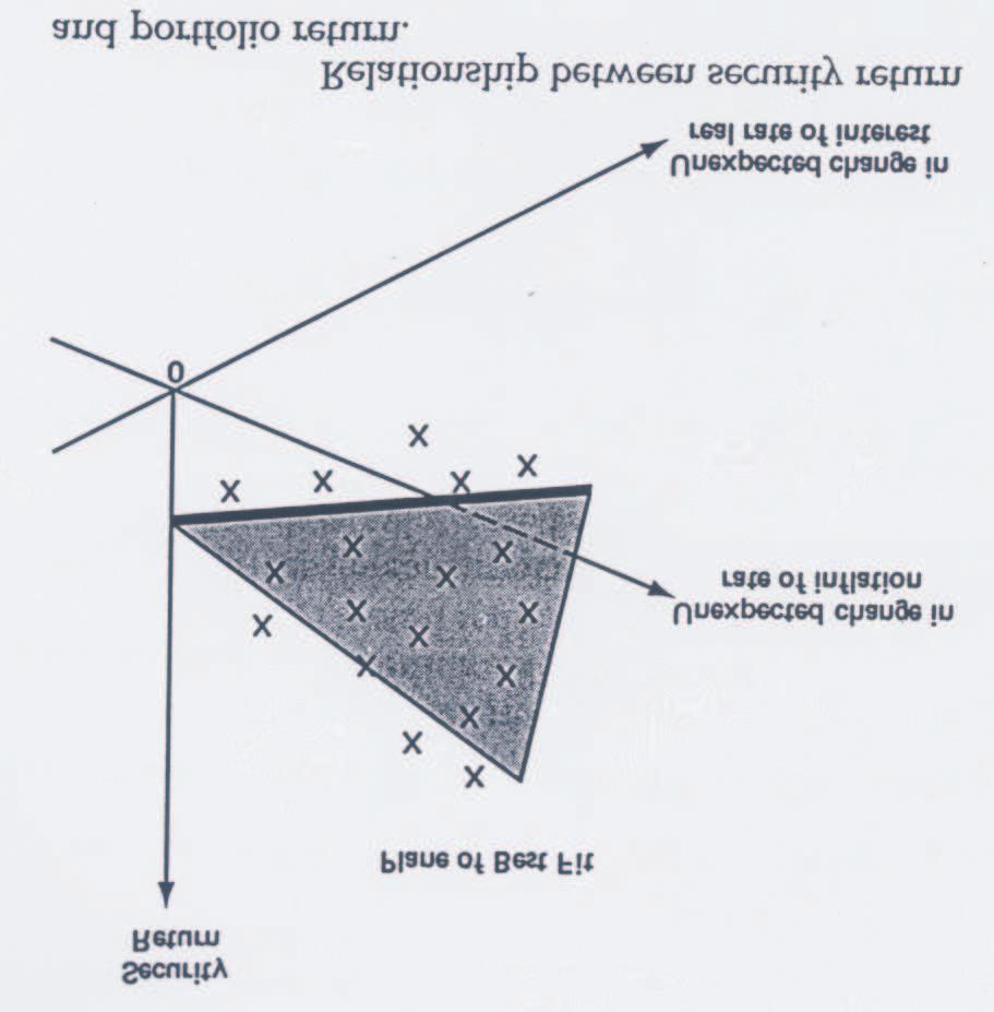
29 3.2 Interpretations and uses of the capital asset pricing model Security market line (SML) From the two relations: r = r f + r M r f σ 2 M σ im r = r f + (r M r f )β i, we can plot either r against σ im or r against β i. 29

30 Under the equilibrium conditions as assumed by the CAPM, every asset should fall on the SML. The SML expresses the risk reward structure of assets according to the CAPM. Point O represents an under-priced security. This is because the expected return is higher than the return with reference to the risk. In this case, the demand for such security will increase and this results in price increase and lowering of expected return. 30

31 Suppose we write the random rate of return of asset i formally as r i = r f + β i (r M r f ) + ǫ i. The CAPM tells us something about ǫ i. (i) Taking the expectation on both sides E[r i ] = r f + β i (r M r f ) + E[ǫ i ] while r i = r f + β i (r M r f ) so that E[ǫ i ] = 0. (ii) Taking the covariance of r i with r M cov(r i, r M ) = so that zero {}}{ cov(r f, r M )+β i + cov(ǫ i, r M ) cov(ǫ i, r M ) = 0. }{{} zero cov(r M, r M ) cov(r f, r M ) 31

32 (iii) Consider the variance of r i so that var(r i ) = βi 2 cov(r M r f, r M r f ) + var(ǫ i ) }{{} var(r M ) σ 2 i = β2 i σ2 M + var(ǫ i). Decomposition of risk Systematic risk = βi 2σ2 M, this risk cannot be reduced by diversification because every asset with nonzero beta contains this risk. Non-systematic (idiosyncratic or specific) risk = var(ǫ i ), this risk is uncorrelated with the market and can be reduced by diversification. 32

33 Portfolios on the CML efficient portfolios Consider a portfolio formed by the combination of the market portfolio and the risk free asset. This portfolio is an efficient portfolio (one fund theorem) and it lies on the CML with a beta value equal to β 0 (say). Its rate of return can be expressed as r p = (1 β 0 )r f + β 0 r M = r f + β 0 (r M r f ) so that ǫ p = 0. The portfolio variance is β0 2σ2 M. This portfolio has only systematic risk (zero non-systematic risk). Suppose the portfolio lies both on the SML and CML, then SML : r p = r f + β(r M r f ) CML : r p = r f + r M r f σ M β = ρ pmσ M σ p σ 2 M σ p = σ p σ M ρ pm = 1. 33

34 Portfolios not on the CML non-efficient portfolios For other portfolios with the same value of β 0 but not lying on the CML, they lie below the CML since they are non-efficient portfolios. With the same value of β 0, they all have the same expected rate of return given by r = r f + β 0 (r M r f ) but the portfolio variance is greater than β0 2σ2 M. The extra part of the portfolio variance is var(ǫ p ). 34

35 equation of CML: r = r f + r M r f σ σ M 35

36 Note that ǫ i is uncorrelated with r M as revealed by cov(ǫ i, r M ) = 0. The term var(ǫ i ) is called the non-systematic or specific risk. This risk can be reduced by diversification. Consider Let β PM = µ P = n i=1 σ 2 P = n n i=1 i,j=1 w i r i = n i=1 (1 β im )w i r f + w i w j β im β jm σ 2 M + n w i β im and α P = n i=1 i=1 µ P = α P + β PM µ M n = β2 PM σ2 M + σ 2 P n i=1 w 2 i σ2 ǫ i. β im w i r M w i (1 β im )r f, then i=1 w 2 i σ2 ǫ i. 36

37 Suppose we take w i = 1/n so that σp 2 = β2 PM σ2 M + 1 n n 2 σǫ 2 i = βpm 2 σ2 M + σ2 /n, i=1 where σ 2 is the average of σ 2 ǫ 1,, σ 2 ǫ n. When n is sufficiently large σ P n i=1 w i β im σ M = β PM σ M. From σ 2 i = β2 im σ2 M +σ2 ǫ i, the contribution from σ 2 ǫ i to the portfolio variance goes to zero as n. 37

38 Example Consider the following set of data for 3 risky assets, market portfolio and risk free asset: portfolio/security σ ρ im β actual expected rate of return = E[P 1 + D 1 ] 1.0 P % % 2 20% % 3 20% % market portfolio 20% % risk free asset % P 1 is the price at time 1 and D 1 is the dividend paid at time 1, both are random quantities. 38

39 Use of CML The CML identifies expected rates of return which are available on efficient portfolios of all possible risk levels. Portfolios 2 and 3 lie below the CML. The market portfolio, the risk free asset and Portfolio 1 all lie on the CML. Hence, Portfolio 1 is efficient while Portfolios 2 and 3 are non-efficient. At σ = 10%, r = 10% }{{} +10% }{{} r f σ (16 10)% 20% }{{} (r M r f )/σ M = 13%. At σ = 20%, r = 10% + 20% (16 10)% 20% = 16%. 39

40 Use of the security market line (SML) The SML asks whether the portfolio provides a return equal to what equilibrium conditions suggest of the amount that should be earned. 40

41 Impact of ρ im Portfolio 1 has unit value of ρ im, that is, it is perfectly correlated with the market portfolio. Hence, Portfolio 1 has zero nonsystematic risk. Portfolios 2 and 3 both have ρ im less than one. Portfolio 2 has ρ im closer to one and so it lies closer to the CML. The expected rates of return of the portfolios for the given values of beta are given by r 1 = r 3 = 10% }{{} +0.5 }{{} r f β (16% 10% }{{} r M r f ) = 13% r 2 = 10% (16% 10%) = 15.4%. These expected rates of return suggested by the SML agree with the actual expected rates of return. Hence, each investment is fairly priced. 41

42 Summary The CAPM predicts that the excess return on any stock (portfolio) adjusted for the risk on that stock (portfolio) should be the same E[r i ] r f β i = E[r j] r f β j. Recall the somewhat restrictive assumptions of the standard CAPM all agents have homogeneous expectations agents maximize expected return relative to the standard deviation agents can borrow or lend unlimited amounts at the riskfree rate the market is in equilibrium at all times. In real world, it is possible that over short periods the market is not in equilibrium and profitable opportunities arises. 42

43 CAPM as a pricing formula Suppose an asset is purchased at P and later sold at Q. The rate of return is Q P, P is known and Q is random. Using the CAPM, P Q P P = r f + β(r M r f ) so that P = 1 The factor 1 + r f + β(r M r f ) discount rate. Q 1 + r f + β(r M r f ). can be regarded as the risk adjusted 43

44 Example (Investment in a mutual fund) A mutual fund invests 10% of its funds at the risk free rate of 7% and the remaining 90% at a widely diversified portfolio that closely approximates the market portfolio, and r M = 15%. The beta of the fund is then equal to 0.9. Suppose the expected value of one share of the fund one year later is $110, what should be the fair price of one share of the fund now? According to the pricing form of the CAPM, the current fair price $110 of one share = 1 + 7% (15 7)% = $ = $

45 Linearity of pricing? ( Q Note that β = cov P 1, r M then have so that 1 = ) / σm 2 so that β = cov(q, r M). We Q P(1 + r f ) + cov(q, r M )(r M r f )/σ 2 M P = r f [ Q cov(q, r M)(r M r f ) σ 2 M ]. Pσ 2 M The bracket term is called the certainty equivalent of Q. In this form, the linearity of Q is more apparent! Note that the riskfree 1 discount factor is applied. Net present value is 1 + r f P r f [ Q cov(q, r M)(r M r f ) σ 2 M ]. 45

46 3.3 Factor models Difficulties associated with the implementation of the CAPM 1. Application of the mean-variance theory requires the determination of the parameter values: mean values of the asset returns and the covariances among them. Suppose there are n assets, n(n 1) then there are n mean values, n variances and covariances. For example, when n = 1,000, the number of parameter 2 values required = 501, In the CAPM, there is really only one factor that influences the expected return, namely, the covariance between the asset return and the return on the market portfolio. 46

47 The assumption of investors utilizing a mean variance framework is replaced by an assumption of the process generating security returns. Merit of the Arbitrage Pricing Theory (APT) 1. APT requires that the returns on any stock be linearly related to a number of factors. It implies that the return on a security can be broken down into an expected return and an unexpected (or surprise) component. 2. Randomness as displayed by the returns of n assets can be traced back to a smaller number of underlying basic sources of randomness (factors). Hopefully, this leads to a simpler covariance structure. 47

48 Specifying the influences affecting the return-generating process 1. Inflation Inflation impacts both the level of the discount rate and the size of the future cash flows. 2. Risk premia Differences between the return on safe bonds and more risky bonds are used to measure the market s reaction to risk. 3. Industrial production Changes in industrial production affect the opportunities facing investors and the real value of cash flow. 48

49 Single-factor model Rates of return r i and the factor are related by r i = a i + b i f + e i i = 1,2,, n. Here, f is a random quantity, a i and b i are fixed constants, e i s are random errors (without loss of generality, take E[e i ] = 0 since any non-zero mean can be absorbed by a i ). Further, we assume We can deduce E[(f f)e i ] = 0 and E[e i e j ] = 0, i j. cov(e i, f) = E[e i f] E[e i ]E[f] = 0. The variances of e i s are known, which are denoted by σ 2 e i. Let b i be the factor loading, which measures the sensitivity of the return to the factor. 49

50 Different data sets (past one month or two months data) may lead to different estimated values. r i = a i + b i f σi 2 = b 2 i σ2 f + σ2 e i σ ij = b i b j σf 2, i j b i = cov(r i, f)/σ 2 f. Only a i s, b i s, σe 2 i s, f and σf 2 parameters. are required. There are (3n + 2) 50

51 Portfolio parameter Let w i denote the weight for asset i, i = 1,2,, n. The portfolio rate of return is r p = n i=1 w i a i + so that r p = a + bf + e, where a = n i=1 w i a i, b = n i=1 n i=1 w i b i f + n i=1 w i b i and e = w i e i n i=1 w i e i. Further, since E[e i ] = 0, E[(f f)e i ] = 0 so that E[e] = 0 and E[(f f)e] = 0; e and f are uncorrelated. Also, σ 2 e = Overall variance of portfolio = σ 2 p = b 2 σ 2 f + σ2 e. n i=1 w 2 i σ2 e i. For simplicity, we take σ 2 e i = S 2 and w i = 1/n so that σ 2 e = S2 n. 51

52 As n, σe 2 0. The overall variance of portfolio σp 2 tends to decrease as n increases since σe 2 goes to zero, but σ2 p does not go to zero since b 2 σf 2 remains finite. The risk due to e i is said to be diversifiable since its contribution to overall risk is essentially zero in a well-diversified portfolio. This is because e i s are independent and so each can be reduced by diversification. The risk due to b i f is said to be systematic since it is present even in a diversified portfolio. 52

53 CAPM as a factor model Express the model in terms of excess returns r i r f and r M r f. r i r f = α i + β i (r M r f ) + e i. With e i = 0, this corresponds to the characteristic line Taking the expectation on both sides r i r f = α i + β i (r M r f ). (1) r i r f = α i + β i (r M r f ). With α i = 0, the above relation reduces to the CAPM. We assume that e i is uncorrelated with the market return r M. 53

54 The characteristic line is more general than the CAPM since it allows α i to be non-zero. The factor model does not assume any utility function or that agents consider only the mean and variance of prospective portfolios. Remarks 1. The presence of non-zero α i can be regarded as a measure of the amount that asset i is mispriced. A stock with positive α i is considered performing better than it should. 2. The general CAPM model is based on an arbitrary covariance structure while the one-factor model assumes very simple covariance structure. 54

55 Single-factor, residual-risk-free models Assume zero idiosyncratic (asset-specific) risk, r i = a i + b i f, i = 1,2,, n, where f is taken that satisfies E[f] = 0 so that r i = a i. Consider two assets which have two different b i s, what should be the relation between their expected returns under the assumption of no arbitrage? Consider a portfolio with weight w in asset i and weight 1 w in asset j. The portfolio return is r p = w(a i a j ) + a j + [w(b i b j ) + b j ]f. 55

56 By choosing w = b j b j b i, the portfolio becomes riskfree and r p = b j(a i a j ) b j b i + a j. This must be equal to the return of the riskfree asset, denoted by r 0. We write the relation as a j r 0 b j = a i r 0 b i = λ. Hence, r i = r 0 + b i λ, where λ is the factor risk premium. Here, λ represents the expected excess return above the riskfree rate per unit of risk (as quantified by f). Note that when two assets are hedgeable, they have the same factor risk premium. set 56

57 Example 1 (Four stocks and one index) Historical rates of return for four stocks over 10 years, record of industrial price index over the same period. Estimate of r i is r i = k=1 var(r i ) = 1 9 r k i. 10 cov(r i, f) = 1 9 k=1 10 (r k i r i ) 2 k=1 (r k i r i )(f k f). Once the covariances are estimated, b i and a i are obtained: b i = cov(r i, f) var(f) and a i = r i b i f. 57

58 We estimate the variance of the error under the assumption that these errors are uncorrelated with each other and with the index. The formula to be used is var(e i ) = var(r i ) b 2 i var(f). Unfortunately, the error variances are almost as large as the variances of the stock returns. There is a high non-systematic risk, so the choice of this factor does not explain much of the variation in returns. Further, cov(e i, e j ) are not small so that the errors are highly correlated. We have cov(e 1, e 2 ) = 44 and cov(e 2, e 3 ) = 91. Recall that the factor model was constructed under the assumption of zero error covariances. 58

59 Year Stock 1 Stock 2 Stock 3 Stock 4 Index aver var cov b a e-var The record of the rates of return for four stocks and an index of industrial prices are shown. The averages and variances are all computed, as well as the covariance of each with the index. From these quantities, the b i s and the a i s are calculated. Finally, the computed error variances are also shown. The index does not explain the stock price variations very well. 59

60 Two-factor extension Consider the two-factor model r i = a i + b i1 f 1 + b i2 f 2, i = 1,2,, n, where the factor f 1 and f 2 are chosen such that E[f 1 f 2 ] = 0, E[f 2 1 ] = E[f2 2 ] = 1, E[f 1] = E[f 2 ] = 0. We assume 1, b 1 = b 11 b 21 b 31 and b 2 = b 12 b 22 b 32 to be linearly independent. Form the portfolio with weights w 1, w 2 and w 3 so that r p = 3 i=1 w i a i + f w i b i1 + f 2 w i b i2. i=1 i=1 60

61 Since 1, b 1 and b 2 are independent, the following system of equations b 11 b 21 b 31 b 12 b 22 b 32 w 1 w 2 w 3 = always has unique solution. In this case, the portfolio becomes riskfree so or r p = 3 i=1 3 i=1 w i a i = r 0 (a i r 0 )w i =

62 Hence, there is a non-trivial solution to a 1 r 0 a 2 r 0 a 3 r 0 b 11 b 21 b 31 b 12 b 22 b 32 w 1 w 2 w 3 = The above coefficient matrix must be singular so that a i r 0 = λ 1 b i1 + λ 2 b i2 for some λ 1 and λ 2. The risk premium on asset i is a i r 0. Absence of riskfree asset r i r 0 = λ 1 b i1 + λ 2 b i2, i = 1,2,, n. If no riskfree asset exists naturally, then we replace r 0 by λ 0. Once λ 0, λ 1 and λ 2 are known, the expected return of an asset is completely determined by the factor loadings b i1 and b i2. Theoretically, a riskless asset can be constructed from any three risky assets so that λ 0 can be determined

63 Prices of risk, λ 1 and λ 2 interpreted as the excess expected return per unit risk associated with the factors f 1 and f 2. Given any two portfolios P and M with b P1 b M1, we can b P2 b M2 solve for λ 1 and λ 2 in terms of the expected return on these two portfolios: r M r 0 and r P r 0. One can show that where r i = r 0 + b i1 (r M r 0 ) + b i2 (r P r 0 ) b i1 = b i1b P2 b i2 b P1 b M1 b P2 b M2 b P1, b i2 = b i2b M1 b i1 b M2 b M1 b P2 b M2 b P1. 63

64 Linkage between CAPM and factor model Consider a two-factor model r i = a i + b i1 f 1 + b i2 f 2 + e i, the covariance of the rate of return of the i th asset with that of the market portfolio is given by cov(r M, r i ) = b i1 cov(r M, f 1 ) + b i2 cov(r M, f 2 ) + cov(r M, e i ). It is reasonable to ignore cov(r M, e i ) if the market represents a welldiversified portfolio. 64

65 We write the beta of the asset as β i = cov(r M, r i ) σ 2 M = b i1 cov(r M, f 1 ) σ 2 M }{{} β f1 cov(r + b M, f 2 ) i2 σm 2. }{{} β f2 The factor betas β f1 and β f2 do not depend on the particular asset. The weight of these factor betas in the overall asset beta is equal to the factor loadings. In this framework, different assets have different betas corresponding to different loadings. 65

66 Example 2 Assume that a two factor model is appropriate, and there are an infinite number of assets in the economy. The cross-sectional relationship between expected return and factor loadings indicates that the price of factor 1 is 0.15, and the price of factor 2 is 0.2. You have estimated factor loadings for stocks X and Y as follows: b 1 b 2 Stock X Stock Y Also, the expected return on an asset having zero betas (with respect to both factors) is What are the approximate equilibrium returns on each of the two stocks? 66

67 Solution The expected return of an asset based on a two-factor model is given by r i = λ 0 + λ 1 b i1 + λ 2 b i2. Here, λ 0 = zero-beta return = 0.05 λ 1 = 0.15 and λ 2 = 0.2. Now, r 1 = λ 0 + λ 1 b 11 + λ 2 b 12 = = 01.8; r 2 = λ 0 + λ 1 b 21 + λ 2 b 22 = =

68 Example 3 Assume that a three-factor model is appropriate, and there are an infinite number of assets. The expected return on a portfolio with zero beta values is 5 percent. You are interested in an equally weighted portfolio of two stocks, A and B. The factor prices are indicated in the accompanying table, along with the factor loadings for A and B. Compute the approximate expected return of the portfolio. Factor i b ia b ib Factor Prices

69 Solution: By APT, the expected return of a portfolio is given by r p = λ 0 + λ 1 b P1 + λ 2 b P2 + λ 3 b P3. Here, λ 0 = 5%, b P1 = 2 1 (b 1A + b 1B ) = 1 2 ( ) = 0.4, b P2 = 1 2 (b 2A + b 2B ) = 1 ( ) = 0.4, 2 b P3 = 1 2 (b 3A + b 3B ) = 1 ( ) = Given λ 1 = 0.07, λ 2 = 0.09, λ 3 = 0.02, so r P = 5% = 13.1%. 69

70 Example 4 Stocks 1 and 2 are affected by three factors, as shown here. Factor 2 and 3 are unique to each stock. Expected values of each are E(F 1 ) = 3.0%, E(F 2 ) = 0.0%, and E(F 3 ) = 0.0%. Neither stock pays a dividend, and they are now selling at prices P 1 = $40 and P 2 = $10. You expect their prices in a year to be E(P 1 ) = $45 and E(P 2 ) = $ R 1 = 6.0( F 1 ) + 0.3( F 2 ) + 0.0( F 3 ) R 2 = 1.5( F 1 ) + 0.0( F 2 ) + 0.4( F 3 ) a. What do factors 2 and 3 reflect? In the context of a broadly diversified portfolio, should the weights 0.3 and 0.4 be positive, as they are shown? b. Neglecting F 2 and F 3, create a riskless arbitrage. c. Relate the return equations to the CAPM. 70

71 Solution a. Factors 2 and 3 appear to be firm specific factors in that they affect only a single stock. Across a large number of stocks, these factors will net to zero. b. By APT, the expected returns of Stock 1 and Stock 2 are r 1 = 6F 1 = 18%, r 2 = 1.5F 2 = 4,5%. The market expected returns are r 1,market = = 12.5%; r 2,market = = 7%. The arbitrage strategy is to short 1/4 unit of Stock 1 and buy one unit of Stock 2. The portfolio is riskless but the expected return = % + 7% = 4.875%. 4 c. Here, r i = 0 + β i F 1 ; while CAPM gives r i = r f + β i (r M r f ). These correspond to r f = 0 and F 1 = r M. 71

72 3.4 Performance indexes Risk-adjusted performance measures based on CAPM We compute some performance indexes which could help assess actual investment performance of different mutual fund managers. Such an index would have to measure the actual returns of traders relative to some equilibrium risk-return relationship. A fund manager may perform better than portfolios on the CML (trading based on the publicly available information) by trading on private information depth: magnitude of the excess return captured by the fund manager breadth: number of different securities for which a fund manager can capture excess return 72

73 Jensen index r _ X Jensen index SML M( =1) r f The Jensen index J uses the SML as a benchmark. It measures the height above the SML. J = r p [r f + (r M r f )β p ] where β p is the beta of the portfolio and r p is the expected rate of return of the portfolio. 73

74 selectivity = net selectivity + diverification Jensen index measures the depth captured by comparing return with the same β (the portfolio may have high σ 2 p with moderate β 2 pσ 2 m) while the total risk measures the depth and breadth. The Jensen index is sensitive to depth but not breadth. The term r f + (r M r f )β p represents the expected return if the portfolio were positioned on the SML. 74

75 According to the CAPM, a fund manager could obtain any point along the SML by investing in the market portfolio and mixing this with the riskless asset to obtain the desired level of β. If the fund manager s choice is to actively manage the fund, then we measure the difference in return between active management and the passive management of investing in the market portfolio and riskless asset. Empirical studies based on Jensen s performance index Out of more than 250 mutual funds, only 9 out-performed an unmanaged S & P 500 index. 75

76 Turn around the argument, J can be used to test the validity of the CAPM. If we find a security with a non-zero Jensen index, then this indicates that the market is not efficient. The CAPM formula is often applied to new financial instruments or projects that are not traded, which are not part of the portfolio. In this case, J can be a useful measure. 76

77 Sharpe index The Sharpe index uses the capital market line (CML) as the benchmark. It is an excess return to variability measure: r _ CML M ABC r f S = r p r f σ p 77

78 The sample estimate of the Sharpe index is Ŝ = r p r f σ p. S is sensitive to both breadth and depth since σ p is a measure of the full risk of the fund. 78

79 Treynov index Risk premium earned per unit of risk taken, where risk is measured in terms of β p. T p = r p r f β p. 79

80 Under the CAPM, the Treynor index should be the same for all portfolios of securities when the market is in equilibrium. If T i of a fund exceeds that of the market portfolio, then the fund is earning an abnormal return relative to that given by the CAPM. Note that J i > 0 iff T i > 0. Further, (i) T i > T j if J i = J j and β i < β j ; (ii) J j > T i if T i = T j and β j > β i. 80

81 Consider two funds Alpha and Omega, both of which have excess expected rate of return of 2% above the SML. Alpha has lower value of beta so that it has a greater excess rate of return per unit of risk. Assume that we can borrow at the riskfree rate r f, we can lever a position in Alpha fund to a position at A by selling the riskfree bond and using the proceed to invest in Alpha. 81

82 Example The data given below are the rate of return achieved by the ABC fund, S & P 500 (as proxy for the market portfolio) and Treasury bill (as the riskless asset) over 10-year period. ABC Fund Performance Rate of return percentages Year ABC S & P T-bills Average Standard deviation Geometric mean Cov(ABC, S & P) Beta Jensen Sharpe

83 Calculation steps 1. Given r i, i = 1,2,, n, the average rate of return is r = 1 n n r i i=1 which serves as an estimate of the true expected return r. The estimate of the average variance is sample variance = ŝ 2 = 1 n 1 n i=1 ( ri r i ) Calculate an estimate of the covariance of the fund and the S & P 500 (proxy for the market portfolio) cov(r, r M ) = 1 n 1 The beta is obtain by n i=1 β = cov(r, r M) var(r M ). (r i r)(r Mi r M ). 83

84 β ABC = = S ABC = r ABC r f ŝ ABC = = Note that the calculated Jensen index for the S & P 500 must be zero. Based on the CAPM, all securities and portfolios should have zero Jensen index value. A positive value of J (as exhibited by the ABC fund) presumably implies that the fund did better than the CAPM prediction (based on the use of a finite data set). 84

85 Sharpe ratio versus Treynor index An investor choosing a mutual fund to represent a large part of her wealth would like to be concerned with the full risk of the fund and σ P is a measure of that risk Sharpe index is more appropriate as the performance index. Look at the other side of the coin, the pension fund of a large corporation may allocate more than 100 fund managers for management. The contribution to the risk of the pension fund as a whole from the portfolio of any of these managers is primarily the non-diversifiable risk. In this case, the Treynor index (which uses β as the risk parameter) is more appropriate to serve as the performance index. 85

86 Decomposition of overall evaluation 86

87 1. Portfolios A and A have the same beta and thus have the same non-diversifiable risk. Since portfolio A lies on the SML, all the risk of portfolio A is completely non-diversifiable. For portfolio A, in the process of earning extra return, diversifiable risk was incurred. 2. Is the extra return worth the extra risk? Compare a naive portfolio with the same total risk as that of portfolio A. This is portfolio A. 3. R A R A = R A R A }{{} net selectivity + R A R A. }{{} diversification 87

88 4. How to decompose R R R F, which is the extra return earned on the naive portfolio for bearing risk? Let β F be the target risk level that the investor is willing to bear. R A R F = R T R F }{{} return from investor s risk + R A R T }{{} return from manager s risk + R A R A }{{} return from selectivity 88

89 Mutual fund performance How much of the risk incurred by the portfolio is due to market movements and how much is due to unique movements of the individual securities in the portfolio? Most mutual funds are well diversified and the majority of the risk they incur is the risk of market movement. However, mutual funds also bear non-market risk. Empirical evidence showed that most mutual funds do not earn sufficient return to justify incurring this extra risk. 89

90 Triumph of Index Tracking Most investors, both institutional and individual, will find that the best way to own common stocks is through an index fund that charges minimal fees. Passive investment management or index tracking certainly has impressive credentials. John C. Bogle, the founder of the Vanguard Group of Investment Companies and an early proponent of the approach has calculated that the S&P 500 Index outperformed the average U.S. equity mutual fund by 3.4 percent per year over the 10 years to December 31, The degree of annual outperformance over five and 15 years was even greater 5.0 percent and 4.0 percent, respectively. 90

91 How to explain the apparent inability of investment professionals to consistently beat the market? Money-management sector is now dominated by professionals. This severely limits the opportunities for outperformance. Active management is generally much more expensive than index tracking costs of employment of investment professionals transaction costs brokers commissions 91

92 Active management still has a role? There is considerable evidence to show that over the long term a diversified portfolio of equities will outperform every other asset class on a risk-adjusted basis. But over shorter periods investors can face the prospect of shortterm losses. Actively managed portfolios can in theory at least reduce these risks. Smart managers can employ many strategies to preserve capital if they foresee a severe market decline. Investments can be sold for cash or hedging strategies can be employed to safeguard the value of the underlying portfolio. 92

93 Measuring performance using the APT Using the APT, the relationship between the factor betas and the expected rates of return on a portfolio is given by r P = r Z + λ 1 β 1,P + + λ n β n,p that is, expected portfolio return = zero-beta portfolio return + sum of factor risk premium Once we have obtained estimates of r Z and λ i s, we can use the above relationship as a benchmark. 93

94 94

95 The slopes of the plane going down each axis represent the sensitivity of the security s return to changes in the two factors (hence, they are estimates of the factor betas). Steps 1. Decide on the factors needed to account for the covariance between stocks. 2. Estimate the factor betas for a cross-section of securities (see the figure where we slide a plane of best fit through the data points). 3. Estimation of the factor prices This is done by relating the estimated factor betas to the average rates of return on each stock. 95

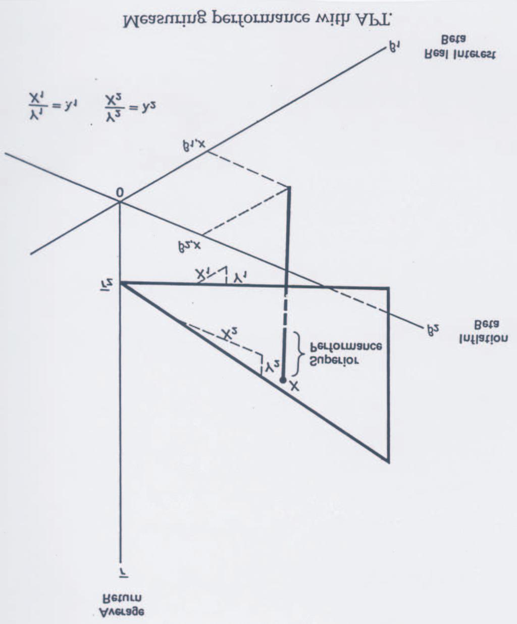
96 96

97 The slope of the plane relative to each horizontal axis serves as the estimate of each factor price. Remark The APT really makes no prediction about what the factors are. Given the freedom to select factors, one can literally make the performance of the portfolio anything you want it to be. 97