Microéconomie de la finance

Transcription

1 Microéconomie de la finance 7 e édition Christophe Boucher christophe.boucher@univ-lorraine.fr 1

2 Chapitre 6 7 e édition Les modèles d évaluation d actifs 2

3 Introduction The Single-Index Model - Simplifying MV optimisation CAPM: Equilibrium model - One factor, where the factor is the excess return on the market. - Based on mean-variance analysis Arbitrage Pricing Theory (APT) - Empirical factors 3-4 CAPM - Beta is dead - Style analysis

4 Part 6. Asset Pricing Models 6.1 MV Optimization Pitfalls 6.2 Single-Index Model 6.3 CAPM 6.4 APT and Multi-Factor Models

5 6.1 MV Optimization Pitfalls

6 Three-Security Portfolio r p = W 1 r 1 + W 2 r 2 + W 3 r 3 s 2 = W 2 p 12 s 12 + W 22 s W 32 s W 1 W 2 Cov(r 1,r 2 ) + 2W 1 W 3 Cov(r 1,r 3 ) + 2W 2 W 3 Cov(r 2,r 3 )

7 In General, n-security Portfolio r p = Weighted average of the n-securities returns s 2 p = Own variance terms + all pair-wise covariances

8 MV Optimization Example Input Data for Asset Allocation Expected return, volatility, correlations

9 MV Optimization Results Efficient frontier with riskless lending and borrowing, and short sales allowed Diversification benefits are substantial

10 Pitfalls with the MV Optimisation Need large amount of input data Expected return, volatility, correlations Estimated portfolio weights are sensitive to estimation errors Small changes in mean returns have large effects on the efficient portfolio weights (Jorion, 1991) How long past time-period is necessary for the estimation? Volatility and correlations change over time, add predictions Static model, without considering rebalancing Transaction costs such as bid-ask spreads, price pressure (market impact), and brokerage fees should be considered.

11 Too many inputs for MV Analysis Expected return: E(R p ) = i w i E(R i ) N expected returns for N assets Std. Dev : p2 = i w i2 i2 + i j,i j w i w j i j ij N variances for N assets N(N-1) correlations for N assets Actually, we need N(N-1)/2 correlations since ij = ji For example, it amounts to 19,900 correlations for 200 assets Altogether, we need 2N+N(N-1)/2 estimates for the MV analysis Most of security analysts focus on estimating expected returns and variance for a limited number of securities. Pair-wise correlations across all assets have to be estimated from some kinds of models, which we are searching for The simplest model is the single-index model

12 6.2 The Single Index Model

13 Single Index Model: Individual Asset s Expected return Assuming that the market index is a common factor describing stock returns - We write stock returns as in the following form: (r i r f ) = i + i (r m r f ) + e i, or R i = i + i R m + e i where E(e i ) = 0 assumed. - This relates stock returns to the returns on a common factor, such as the S&P 500 Stock Index,

14 Single Index Model: Two Components It divides stock returns into two components A market-related part, i R m i measures the sensitivity of a stock to market movements A non-market-related or unique part, i + e i Therefore, expected return can be written as, E(R i ) = i + i E(R m )

15 Single Index Model: Systematic Risk & Unsystematic Risk It also divides a security s variance (total risk) into market risk & unique risk i2 = i2 m2 + ei 2 - This is obtained from taking variance operator on both sides of the single index model: Var (R i ) = Var( i + i R m + e i ) i2 = i2 m2 + ei 2.- From this, we see the following holds: i2 m 2 / i2 = 1- ei2 = i,m 2 Systematic Risk / Total Risk = i,m 2

16 Single Index Model: Individual Asset s Covariance If securities are related only in their response to the market: - Securities covary together, only because of their relationship to the market index, and thus, - Security covariances depend only on market risk: ij = i j m 2

17 Single Index Model: Individual Asset s Covariance ij = i j m 2 which is obtained as in the following: ij = E{[R i E(R i )][R j E(R j )]} = E{[( i + i R m + e i ) ( i + i E(R m ))] [( j + j R m + e j ) ( j + j E(R m ))]} = E{[ i (R m E(R m ) + e i ][ j (R m E(R m ) + e j ]} = i j E[R m E(R m )] 2 + i E[e j (R m E(R m ))] + j E[e i (R m E(R m ))] + E(e i e j ) = i j m 2 Note that E[e j R m ] = 0 and E(e i e j ) = 0 assumed above

18 Number of inputs for the MV Analysis Now, we need the following inputs for the MV analysis: E(R i ) = i + i E(R m ) i2 = i2 m2 + ei 2 ij = i j m 2 - That is, we need N i s, N i s, 1 E(R m ), 1 m2, and N ei2, which are 3N+2 estimates, instead of 2N+N(N-1)/2 without an index model

19 Advantage of the Single Index Model Reduces the number of inputs for portfolio optimization. Example: 50 (N) stocks, how many inputs? Expected Returns 50 N Variances 50 N Covariances 50*(50-1)/2=1225 N*(N-1)/2 Total 1325 N*(N+3)/2

20 Number of inputs for portfolio optimization Inputs required with a single-index model. What is the reduction in number of inputs? Expected (Excess) Returns 50 N betas 50 N Firm specific risk 2 (e i ) 50 N Market risk M Market Excess Returns 1 1 Total 152 3N+2

21 Well-diversified portfolio s Expected return Now, consider a well-diversified portfolio p with N assets: E(R p ) = i w i E(R i ) = i w i [ i + i E(R m )] (by the single index model) = i w i i + i w i i E(R m ) = p + p E(R m ) - This would equal the expected return on the market portfolio if p = 0 and p = 1 Thus, we see that the beta on the market should be 1

22 Well-diversified portfolio s Variance Now, look at the variance of the well-diversified portfolio: p2 = i w i2 i2 + i j,i j w i w j ij = i w i2 [ i2 m2 + ei2 ] + i j,i j w i w j [ i j m2 ] = i j w i w j i j m2 + i w i2 ei 2 = [ i w i i ][ i w j j ] m2 + i w i2 ei 2 = p2 m2 + i w i2 ei 2 p2 m2 = m2 [ i w i i ] 2 - Thus, the contribution of individual asset s risk to the portfolio is only thru i, and residual risk is diversified away by forming the welldiversified portfolio

23 Estimating the Index Model Regression analysis is often used to estimate an index model - Try to fit a best line - Dependent variable (Y): excess return of individual security (portfolio) - Independent variable (X): excess market return.

24 Security Characteristics Line Estimation of Harley's Beta (12/ /2008: 251 obs.) 60% 50% 40% 30% 20% Harley 10% 0% -10% -20% -30% -40% -20% -15% -10% -5% 0% 5% 10% 15% S&P500

25 Estimating the Index Model What is the best line? Minimize the prediction error What is the prediction error? Deviation of data points from predicted data points. We will square the deviations so that the positive deviations and negative deviations do not cancel each other out This estimation method is known as the least squared error (LSE) method.

26 Security Characteristics Line Estimation of Harley's Beta (12/ /2008: 251 obs.) 60% 50% 40% y = 1,3402x + 0,0141 R 2 = 0, % 20% Harley 10% 0% -10% -20% -30% -40% -20% -15% -10% -5% 0% 5% 10% 15% S&P500

27 Regression Results (using DROITEREG in Excel) r r ( r r ) ( r r ) Ha f m f m f Beta alpha SE SE R² SE(Y) F df SS reg SS err R² 1 SS SS err tot SS SS reg tot SS y y 2 tot ( t ) t 2 ( ˆ reg t ) tot reg err t SS y y SS SS SS 2 SS ( ˆ err yt yt ) t

28 Components of Risk Market or systematic risk: - risk related to the macro economic factor or market index. Unsystematic or firm specific risk: - risk not related to the macro factor or market index. Total risk = Systematic + Unsystematic

29 Measuring Components of Risk p 2 = p2 m (e i ) where: p 2 = total variance p2 m 2 = systematic variance 2 (e p ) = unsystematic variance

30 Examining Percentage of Variance Total Risk = Systematic Risk + Unsystematic Risk Systematic Risk/Total Risk = R 2 ß i 2 m 2 / 2 = R 2 2 (e i )/ 2 = 1-R 2

31 Index Model and Diversification Case of An Equally-Weighted Portfolio Return model for Portfolio P Beta for portfolio P Alpha for the portfolio Error term for the portfolio Risk for the portfolio

32 An Example Consider two stocks A & B with the following characteristics. Stock E(R) Beta i (e) A B The market index has a std of 22, and the risk free rate is 8. - What are the stds of stocks A and B? - Hint: first, find the variances ( e ) A A M A ( e ) B B M B

33 An Example (Cont d) Suppose that you were to construct a portfolio with w A =.30, w B =0.45, w f =0.25. What is the expected return of the portfolio? - Expected return on a portfolio is weighted average of returns of individual assets. E(r P ) w A E(r A ) w B E(r B ) w f r f (0.3013) (0.4518) (0.258) 14

34 An Example (Cont d) ) ( ) ( ) ( ) ( f f B B A A P e w e w e w e What is the non-systematic standard deviation of the portfolio? Because covariance between individual asset s nonsystematic risk is zero. We have 2 ( ) ( ) 405 P P e e 0) (0.25 ) 40 (0.45 ) 30 (

35 p wa β A wb β B w f β f An Example (Cont d) What is the standard deviation of the portfolio? - Recall: ( e ) p p M p - Therefore, we need portfolio beta - Beta of a portfolio is a weighted average of individual betas. ( ) ( ) (0.250) P M - We already have 2 (e P ). 2 P 2 P 2 M 2 ( e P )

36 Estimating Beta It is common to estimate the beta from running a regression with past data, and use this historical beta as an estimate for the future beta Problem with the historical beta - Beta estimates have a tendency to regress toward one - Beta may change over time - Adjusting historical beta to get a better forecast of betas or correlations

37 Adjusting Beta Many analysts adjust estimated betas to obtain better forecasts of future betas. Merrill Lynch adjusts beta estimates in a simple way: - Adjusted beta = 2/3 sample beta + 1/3 (1) When using daily or weekly returns, run a regression with lagged and leading market returns. - R it = a i + b 1 R mt-1 + b 2 R mt + b 3 R mt+1 - The estimate of beta is: Beta i = b 1 + b 2 + b 3.

38 Adjusted Beta Contents r i Fundamental Blume Vasicek S i i 0 f f 1 F f u i ˆ ˆ ˆ i i 2 1 t ˆ ˆ i* i 2 i i 2 1 ( 1 ) 1; 2 i i 1 Performance Work for the same industry Average sensitivity of firm Depending on the size of the uncertainty Bias Non-symmetry Upward forecast underestimation Accuracy Property of firm moderate good Fundamental factors: dividend payout, asset growth, leverage, liquidity, asset size, earning variability.

39 Index Model in Practice - Tracking Portfolios A portfolio with the following estimates: R P = R S&P500 + e P Is this portfolio desirable? Anything you could do to profit from your knowledge? Should you buy or sell assets in portfolio P? What if market moves unfavorably?

40 Tracking Portfolios What if market moves unfavorably? - Solution: try to neutralize the market movements. - Take an opposite position in the market portfolio (S&P 500) so that the effect of market movement can be removed. Let s call the opposite position as T. How large should be the beta of T? How to achieve it? in S&P 500. What is weight in T?. Need to take position in T-bill so that the weight in T is 1.0. How much to take? Therefore, the final position of T should be S&P500 + Tbills.

41 Tracking Portfolios What if market moves unfavorably? - Solution: try to neutralize the market movements. - Take an opposite position in the market portfolio (S&P 500) so that the effect of market movement can be removed. Let s call the opposite position as T. How large should be the beta of T? 1.4 How to achieve it? 1.4 in S&P 500. What is weight in T? 1. Need to take position in T-bill so that the weight in T is 1.0. How much to take? -.4 Therefore, the final position of T should be 1.4 S&P Tbills.

42 Tracking Portfolios What return will your combined position of P and T generate? R C =R P -R T =( XR S&P +e P ) 1.4XR S&P = e P Is there any risk in this strategy? This strategy is often called as the Long-short strategy, and is commonly used by many hedge funds! Use futures contracts to hedge your portfolio

43 6.3 CAPM

44 Capital Asset Pricing Model (CAPM) Assumptions Investors are price takers Investors have homogeneous expectations One period model Presence of a riskless asset No taxes, transaction costs, regulations or short-selling restrictions (perfect market assumption) Information is costless and available to all investors. Returns are normally distributed or investor s utility is a quadratic function in returns (MV optimisers)

45 CAPM Derivation Return m Efficient frontier R f p For a well-diversified portfolio, the equilibrium return is: E( Rm R f ) E( R ) R p f p m

46 CAPM Derivation For the individual security, the return-risk relationship is determined by using the following: E( R ) we( R ) (1 w) E( R ) p i m w (1 w) 2 w(1 w) p i m im 1/2 Rp Ri Rm w w p 2w i 2(1 w) m 2 im 4w im p

47 CAPM Derivation At the equilibrium, the excess weight of the security i in the market portfolio is 0, w = 0: R p w w0 2 2 w p m im im m w0 R i R m m m

48 CAPM Derivation The slope of this tangential portfolio at m must equal to: E( R R ) m m Thus : f E( Rm R f ) Rp Rp w E( Ri ) E( Rm ) w 2 m p p w0 im m m Then, we obtain the CAPM: E( R ) R E( R ) R m f i f 2 im m

49 Resulting Equilibrium Conditions All investors will hold the same portfolio for risky assets market portfolio Market portfolio contains all securities and the proportion of each security is its market value as a percentage of total market value.

50 Resulting Equilibrium Conditions (cont d) Risk premium on the market depends on the average risk aversion of all market participants. Risk premium on an individual security is a function of its covariance with the market.

51 The Premium of the Market Portfolio Let s assume that there are 3 investors, with risk aversion parameters A 1, A 2, and A 3. Each has $1 to invest. Recall (session 3; slide 12) that the optimal weight each investor assigns to the risky market portfolio should be: Investor Weight on market portfolio E( R ) R M A M E( R ) R M A M E( R ) R M A M f f f

52 The Premium of the Market Portfolio (cont d) The total money invested in the market portfolio therefore is: E( R ) R E( R ) R E( R ) R A A A M f M f M f M M M E( RM ) R f A1 A2 A3 M

53 The Premium of the Market Portfolio (cont d) What should be the total investment in the market portfolio? Let s take a look at a simple example. Let A 1 =1.5, A 2 =2, A 3 =3, and E(R m )-R f =9%, m =20%. Investor A x* 1-x* % 70% % 77.5% % 85%

54 The Premium of the Market Portfolio (cont d) What if E(R m )-R f =6%, m =20%? Investor A x* 1-x* % 80% % 85% % 90%

55 The Premium of the Market Portfolio (cont d) In a simplified economy, risk-free investment involve borrowing and lending among investors. - Any borrowing must be offset by the lending position i.e. net lending and net borrowing across all investors must be zero. E ( rm ) r f A1 A 2 A 3 M 1 E ( r ) r A M f 2 M Where A is called the (harmonic) average of A 1, A 2, and A 3 1 A A 1 1 A 2 1 A 3

56 The Premium of the Market Portfolio and Risk Aversion Historical market risk premium (proxied by the S&P 500 index) is 8.2% The standard deviation of the market portfolio is 20.6%. Based on these statistics, what is the average coefficient of risk aversion? E( r M ) r f 8.2 A 2 M A A Risk premium (E(R M ) R f ) on the market depends on the (harmonic) average risk aversion of all market participants.

57 Return and Risk For Individual Securities The risk premium on individual securities is a function of the individual security s contribution to the risk of the market portfolio. An individual security s risk premium is a function of the covariance of returns with the assets that make up the market portfolio.

58 Return and Risk For Individual Securities Simplified Derivation For simplicity, let s assume that there are only three assets in the market, then: R w R w R w R M R R w ( R R ) w ( R R ) M f 1 1 f 2 2 f w ( R R ) 3 3 Therefore, the marginal contribution of asset 1 to the expected risk premium of the market portfolio is: f w1 E( R1 ) R f

59 Return and Risk For Individual Securities Simplified Derivation (Cont d) Now, let s look at the variance of the market portfolio R w R w R w R M Var( r ) Cov( R, R ) M M M Cov( w R w R w R, R ) w Cov( R, R ) w Cov( R, R ) w Cov( R, R ) 1 1 M 2 2 M 3 3 M M The marginal contribution of asset 1 to the risk (variance) of the market portfolio is: w1 Cov R1 R M (, )

60 Return and Risk For Individual Securities Simplified Derivation (Cont d) The reward-to-risk ratio for asset 1 therefore is w1 ( E( R1 ) R f ) E( R1 ) R f w Cov( R, R ) Cov( R, R ) 1 1 M 1 M Now, recall that the market reward to risk ratio is: E( R ) R M 2 M f

61 Return and Risk For Individual Securities Simplified Derivation (Cont d) In equilibrium, the reward to risk ratio should be the same for all the assets. - Why? - Therefore, E( R1 ) R E( R ) R Cov( R, R ) 1 M f M f 2 M - since, E( R1 ) R E( R ) R Cov( R, R ) 1 f M f 2 M M Cov( R, R ) E( R ) R E( R ) r 1 M 1 f 2 M f M

62 Return and Risk For Individual Securities Simplified Derivation (Cont d) We call the following ratio as the beta for asset 1. Cov( R, RM ) M The equation for the expected rate of return can be simplified as: E( R ) R E( R ) R 1 f 1 M f E( R ) R E( R ) R 1 f 1 M f We did it! This is the CAPM model

63 Return and Risk For Individual Securities Beta of security i measures how the return of i moves with the return of the market. In other words, it is a measure of the systematic risk. Only systematic risk matters in determining the equilibrium expected return. Unsystematic risk affects only a single security or a limited number of securities. Systematic risk affects the entire market.

64 The Security Market Line (SML) E( R ) R E( R ) R i f i M f SML Expected return M R f Risk Premium E(R M ) R f ) = slope of the SML

65 Examples of SML E(R m ) - R f =.08 R f =.03 - What is the expected return for a security with a beta of 0? - What is the expected return for a security with a beta of 0.6? - What is the expected return for a security with a beta of 1.25?

66 Graph of Sample Calculations R x =13% R M =11% E(R) SML Slope=0.08 R y =7.8% 3% 0 f.6 y x

67 The CAPM and Beta Facts about beta If > 1.0, the security moves more than the market when the market moves If < 1.0, the security moves less than the market when the market moves. So, if > 1.0, the asset has more risk relative to the market portfolio and if < 1.0, the asset is has less risk relative to the market portfolio. Since all risk is measured relative to the market portfolio, the beta of the market portfolio must be 1.0.

68 Alpha and Disequilibrium The difference between the actual expected rate of return and that dictated by the SML is called as alpha. i E( ri ) [ rf i ( E( rm ) rf )] What should alpha be if a security is fairly priced according to CAPM?

69 Disequilibrium Example E(R m ) - R f =.08 R f =.03 - Suppose a security with a of 1.25 is offering expected return of 15%. - According to SML, it should be 13%. - What is the alpha for this security? - Is this security overpriced or underpriced, why?

70 Disequilibrium Example E(R) SML 15% 13% r f =3%

71 Alpha and Security Price What would happen if alpha is positive/negative? When are securities overpriced or underpriced?

72 The Security Market Line and Over- Undervaluation Identifying undervalued and overvalued assets - In equilibrium, all assets and portfolios of assets should fall on the SML. - Therefore, we can compare a security s estimated (or expected) return with its required return from the SML (CAPM) to determine if the asset is overvalued or undervalued.

73 The Security Market Line and Over- Undervaluation Identifying undervalued and overvalued assets If a security s expected return is below its required return, based upon the SML, it is overvalued and If a security s estimated return is above its required return, based upon the SML, it is undervalued.

74 The Security Market Line and Over- Undervaluation CAPM Example Investment Required return Beta Expected Return from CAPM A 14% % B 5% 0 4% C.75 10% D % E %

75 The Security Market Line and Over- Undervaluation CAPM Example Rm = 14%, Rf = 5% Why? See Required returns from the CAPM C: (14-5) = 11.75% D: (14-5) = 25.7% E: (14-5) = 15.8%

76 The Security Market Line and Over- Undervaluation CAPM Example: If we compare required returns to expected returns, investments A and E are undervalued and investments B, C, and D are overvalued. Graphically, this means investments A and E plot above the security market line and investments B, C, and D plot below the security market line.

77 Example of using the SML to identify overvalued and undervalued assets SML Expected return A E D R f C B 1

78 Extensions of CAPM Black s Zero Beta Model CAPM and Liquidity

79 Extensions of CAPM Black s Zero Beta Model - Absence of a risk-free asset - Combinations of portfolios on the efficient frontier are efficient. - All frontier portfolios have companion portfolios that are uncorrelated. - Returns on individual assets can be expressed as linear combinations of efficient portfolios.

80 Efficient Portfolios and Zero Companions E(R) E[R z (Q) ] E[R z (P) ] P Z(Q) Q Z(P) s

81 Zero Beta Market Model Cov( Ri, RM ) E( R ) E( R ) E( R ) E( R ) i Z ( M ) M Z ( M ) 2 M CAPM with E(R z (m) ) replacing R f

82 CAPM & Liquidity Liquidity Illiquidity Premium - If there are two assets with identical expected rate of returns and beta, but one costs more to trade, which asset do you prefer? Research supports a premium for illiquidity. - Amihud and Mendelson - Acharya and Pedersen

83 CAPM with a Liquidity Premium E( R ) R [ E( R ) R ] f ( c ) i f i i f i f (c i ) = liquidity premium for security i f (c i ) increases at a decreasing rate

84 Liquidity and Average Returns Average monthly return(%) Bid-ask spread (%)

85 Empirical tests of the CAPM: Is Beta Dead? Under CAPM, Beta is only risk - Higher ß higher return, & vice versa - Evidence is weak: the relationship between beta and rates of return is a moot point Fix Beta? - Treat as nonstationary Acknowledge other sources of risk? - Size, P/B ratio, skewness, leverage, inflation, momentum (overreactions)

86 Returns to Beta: Is Beta Dead? Mean Beta Monthly Mean Group Return (%) Beta 1 (High) (Low) Average Monthly Returns and Estimated Betas from July 1963 to December 1990 for Ten Beta Groups

87 Returns to Size Mean Size Mean Monthly Group Beta Return (%) 1 (Large) (Small) Average Monthly Returns and Estimated Betas from July 1963 to December 1990 for Ten Size Groups

88 Returns to Fundamental: Price-to-Book Mean Price/Book Monthly Mean Group Return (%) Beta 1 (High) (Low) Average Monthly Returns and Estimated Betas from July 1963 to December 1990 for Ten Price/Book Groups.

89 Returns to Fundamental Screens: Value vs Glamour/Growth high low Growth in sales high Cash-flow-to-price ratio low Value 5-year returns Glamour/ Growth Source: Lakonishok, Shleifer, & Vishny, Contrarian Investment, Extrapolation, and Risk, Journal of Finance, Vol. 49, No. 5. (Dec., 1994), p 1554.

90 Time-varying Beta Siemens-Beta vs. DAX Index between estimated at 1.2 Source: Bloomberg

91 Time-varying Beta Siemens-Beta vs. DAX Index between (bull market) estimated at 0.99 Source: Bloomberg

92 Time-varying Beta Siemens-Beta vs. DAX Index between (bear market) estimated at 1.47 Source: Bloomberg

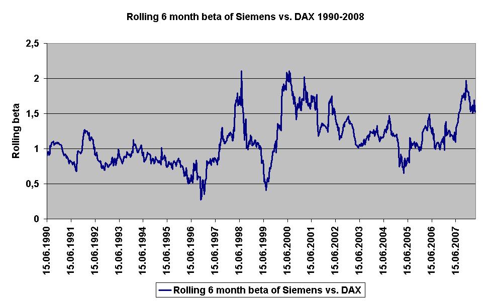
93 Time-varying Beta

94 Alternatives to the CAPM Factor models (APT) - Factor models assume that the return generating process on a security is sensitive to the movement of various factors or indices. - A factor model attempts to capture the major economic forces that systematically move the prices of all securities. Fama-French 3-factor Model (4-5-6 factors)

95 Roll Critique The market portfolio is unobservable so you have to use a proxy So if the CAPM is true, but your proxy is off, you can reject the model. On the other hand if the CAPM is false, but the proxy is meanvariance efficient you can not reject the model So the CAPM is not testable!!!

96 6.4 APT and Multi-Factor Models

97 The APT : Some Thoughts The Arbitrage Pricing Theory New and different approach to determine asset prices. Based on the law of one price : two items that are the same cannot sell at different prices. Requires fewer assumptions than CAPM Assumption : each investor, when given the opportunity to increase the return of his portfolio without increasing risk, will do so. Mechanism for doing so : arbitrage portfolio

98 Arbitrage Portfolio Arbitrage portfolio requires no own funds Assume there are 3 stocks : 1, 2 and 3 X i denotes the change in the investors holding (proportion) of security i, then X 1 + X 2 + X 3 = 0 No sensitivity to any factor, so that b 1 X 1 + b 2 X 2 + b 3 X 3 = 0 Example : 0.9 X X X 3 = 0 (assumes zero non factor risk)

99 Single Factor Model Returns on a security come from two sources Common macro-economic factor Firm specific events Possible common macro-economic factors Gross Domestic Product Growth Interest Rates

100 Single Factor Model Equation r i = E(r i ) + Beta i (F) + e i r i = Return for security I Beta i = Factor sensitivity or factor loading or factor beta F = Surprise in macro-economic factor (e.g. unexpected change in GDP) (F could be positive, negative or zero) e i = Firm specific events

101 Multifactor Models Use more than one factor Examples include gross domestic product, expected inflation, interest rates etc. Estimate a beta or factor loading for each factor using multiple regression.

102 Multifactor Model Equation r i = E(r i ) + Beta GDP (GDP) + Beta IR (IR) + e i r i = Return for security I Beta GDP = Factor sensitivity for GDP Beta IR = Factor sensitivity for Interest Rate e i = Firm specific events

103 Example Example: Beta GDP = 1.2, Beta IR =0.7, E(r i )=0.10 If GDP is revised to be 1% higher than expected, what should be your revised E(r i )? If interest rate is revised to be 1% lower than expected, what should be your revised E(r i )?

104 Example (solution) Example: Beta GDP = 1.2, Beta IR =0.7, E(r i )=0.10 If GDP is revised to be 1% higher than expected, what should be your revised E(r i )? = x 0.01 = If interest rate is revised to be 1% lower than expected, what should be your revised E(r i )? = x 0.01 = 0.093

105 Multifactor SML Models E(r) = r f + GDP RP GDP + IR RP IR GDP = Factor sensitivity for GDP RP GDP = Risk premium for GDP, which is the difference in the expected return of a portfolio ( GDP =1, IR =0) and the risk free rate. IR = Factor sensitivity for Interest Rate RP IR = Risk premium for IR, which is the difference in the expected return of a portfolio ( GDP =0, IR =1) and the risk free rate.

106 Multifactor SML - An Example r f = 4.0% GDP = 1.2 RP GDP = 6% IR = -.3 RP IR = -7% E(r) = r f + GDP RP GDP + IR RP IR = 13.3%

107 Arbitrage Pricing Theory Arbitrage - arises if an investor can construct a zero investment portfolio with a sure profit. Since no investment is required, an investor can create large positions to secure large levels of profit. In efficient markets, profitable arbitrage opportunities will quickly disappear.

108 APT & Well-Diversified Portfolios r P = E (r P ) + P F + e P F = some common factor For a well-diversified portfolio: Systematic risk or factor risk is captured by P, which is the weighted average of betas of individual assets. Unsystematic risks cancel each other out, therefore e P approaches zero, similar to CAPM.

109 Portfolios and Individual Security E(r)% E(r)% F F Portfolio Individual Security

110 Disequilibrium Example E(r)% 10 A 6 r f = 4 C Beta for F

111 Disequilibrium Example Which portfolio is over-valued? What to do with this portfolio? Any portfolio undervalued? Can we buy a fairly priced portfolio instead? How to control for systematic risk? Use funds to construct an equivalent risk higher return Portfolio D. D is composed of A & Risk-Free Asset What are weights of A and RF in Portfolio D? What is the arbitrage profit?

112 Disequilibrium Example E(r)% Create a portfolio D composed of half of portfolio A and half of the risk free rate r f = 4 D C A Beta for F

113 Disequilibrium Example E(r)% Arbitrage portfolio: D - C D has an equal beta but greater expected return r f = 4 D C A Beta for F

114 More Disequilibrium Examples Portfolio E(r) Beta A 12% 1.2 F 6% 0.0 E 8% 0.6 Is there an arbitrage opportunity? Yes. Reward to risk ratios are different. How to arbitrage? ½ A + ½ F (Long or short) E (long or short)

115 More Disequilibrium Examples Portfolio E(r) Beta A 12% 1.2 F 6% 0.0 E 8% 0.6 Is there an arbitrage opportunity? Yes. Reward to risk ratios are different. How to arbitrage? ½ A + ½ F (Long or short) E (long or short)

116 More Disequilibrium Examples Portfolio E(r) Beta X 16% 1.00 Y 12% 0.25 F 8% 0 Is there an arbitrage opportunity? Yes. Reward to risk ratios are different. How to arbitrage? ¼ X + ¾ F (Long or short) Y (long or short)

117 More Disequilibrium Examples Portfolio E(r) Beta X 16% 1.00 Y 12% 0.25 F 8% 0 Is there an arbitrage opportunity? Yes. Reward to risk ratios are different. How to arbitrage? ¼ X + ¾ F (Long or short) Y (long or short)

118 More Disequilibrium Examples What if we do not observe a risk free asset? Portfolio E(r) Beta X 16% 1.25 Y 14% 1.00 Z 8% 0.75 Is there an arbitrage opportunity? How to evaluate? Consider combining two portfolios so that the beta risk of the resulting portfolio is the same as the third portfolio, and compare the expected returns. ½ X + ½ Z (Long or short) Y (long or short)

119 More Disequilibrium Examples What if we do not observe a risk free asset? Portfolio E(r) Beta X 16% 1.25 Y 14% 1.00 Z 8% 0.75 Is there an arbitrage opportunity? How to evaluate? Consider combining two portfolios so that the beta risk of the resulting portfolio is the same as the third portfolio, and compare the expected returns. ½ X + ½ Z (Long or short) Y (long or short)

120 Identifying the Factors Unanswered questions : How many factors? Identity of factors Possible factors (literature suggests : 3 5) Chen, Roll and Ross (1986) Growth rate in industrial production Rate of inflation (both expected and unexpected) Spread between long-term and short-term interest rates Spread between low-grade and high-grade bonds

121 Three approaches to estimate factors Statistical factors Extracted from returns Macroeconomic factors Inflation, term structure, Fundamental factors SMB, HML, etc.

122 Principal Component Analysis (PCA) Technique to reduce the number of variables being studied without losing too much information in the covariance matrix. Objective : to reduce the dimension from N assets or M economics variables to k factors Principal components (PC) serve as factors First PC : (normalised) linear combination of asset returns with maximum variance Second PC : (normalised) linear combination of asset returns with maximum variance of all combinations orthogonal to the first component

123 Pro and Cons of Principal Component Analysis Advantage : Allows for time-varying factor risk premium Easy to compute Disadvantage : interpretation of the principal components, statistical approach

124 APT and CAPM Compared APT applies to well diversified portfolios and not necessarily to individual stocks. With APT it is possible for some individual stocks to be mispriced - not lie on the SML. APT is more general in that it gets to an expected return and beta relationship without the assumption of the market portfolio. APT can be extended to multifactor models.

125 APT and CAPM Compared (Cont d) APT is much robust than CAPM for several reasons: 1. APT makes no assumptions about the empirical distribution of asset returns; 2. APT makes no assumptions on investors utility function; 3. No special role about market portfolio 4. APT can be extended to multiperiod model.

126 Summary APT alternative approach to explain asset pricing Factor model requiring fewer assumptions than CAPM Based on concept of arbitrage portfolio Interpretation : Factor s are difficult to interpret, no economics about the factors and factor weightings.

127 Questions and Problems

128 Exercise 1. Index Model 1. Consider monthly returns on the next slide and calculate: A. Alpha for each stock B. Beta for each stock C. SD of the residuals from each regression D. Correlation coefficient between each security and the market E. Average return of the market F. Variance of the market

129 Exercise 1. Index Model Security Month A B C S&P

130 Exercise 1. Index Model 2. A. Compute the mean return and variance of return for each stock in problem 1 using: (1) The single index model (2) The historical data B. Compute the covariance between each possible pair of stocks using (1) The single index model (2) The historical data C. Compute the return and SD of a 1/N portfolio (equally weighted) using: (1) The single index model (2) The historical data D. Discuss the results

131 Exercise 2. CAPM 1. Assume that the following assets are correctly priced according to the SML. Derive the SML. What is the expected return on an asset with a Beta of two? R 1 = 6% and R 2 = 12% 1 = 0.5 and 2 = Assume the SML given below and suppose that analysts have estimated the Beta of two stocks as follows: x = 0.5 and y = 2. What must the expected return on the two securities be in order for them to be a good purchase? R i = i 3. Assume that over some period a CAPM was estimated. Results are shown below. Assume that over the same period two mutual funds had the following results: R A = 10% and R B = 15% 1 = 0.8 and 2 = 1.2 R i = i What can be said about the fund performance? 4. Consider the CAPM line shown below. What is the excess return of the market over the risk-free rate? What is the risk free rate? Ri = i

132 Exercise 3. APT and Multifactor Models 1. Assume that the following two factor-model describe returns: R i = a i + b i1.i 1 + b i2.i 2 + e i Assume that the following three portfolios are observed: Portfolio Expected Return b i1 b i2 A B C Find the equation of the plane that must describe equilibrium returns 2. Referring to the results of question 1, illustrate the arbitrage opportunities that would exist if a portfolio called D with the following properties were observed: R D = 10 b D1 = 2 b D2 = 0

133 Exercise 3. APT and Multifactor Models 3. Repeat Question 1 if the three portfolios observed have the following characteristics. Portfolio Expected Return b i1 b i2 A B C Referring to the results of Question 3, illustrate the arbitrage opportunities if a portfolio called D with the following properties were observed: R D = 15 b D1 = 1 b D2 = 0

134 Thank you for your attention See you next week