Appendix G TRAVEL DEMAND MODEL DOCUMENTATION

Transcription

1 Appendix G TRAVEL DEMAND MODEL DOCUMENTATION

2 APPENDIX G - TRAVEL DEMAND MODEL DOCUMENTATION 1.0 INTRODUCTION The Memphis Urban Area MPO is developing the Direction Long-Range Transportation Plan (LRTP) for the Memphis region. The horizon year of the Plan is The previous LRTP, approved March 31, 2008, had a horizon year of The Direction 2040 LRTP will use the current Memphis MPO Travel Demand Model (TDM) to forecast the future traffic conditions based on the future land use, demographic and economic growth. The base year for the Direction 2040 LRTP is The current Memphis MPO TDM was completed in 2007 and developed with TransCAD software platform. The model development underwent an extensive review process through a local steering committee, an expert panel review, and a Peer Review Process. The completed model has also been reviewed and approved by the appropriate State Departments of Transportation, Federal Highway Administration (FHWA) and Federal Transit Administration (FTA). The existing TDM has base year of 2004 and a horizon year of 2030 with various interim years of 2008, 2010, 2011, 2014, 2017, and Since 2007, the MPO has maintained and updated the TDM to assist the on-going LRTP and Transportation Improvement Program (TIP) amendment process. To assist the development of the 2040 LRTP using the current travel demand model, the TDM must have the ability to evaluate the future travel demand and transportation network deficiencies for horizon year 2040 and multiple interim years. Although it would be ideal to update the TDM's base year to 2010, the MPO will postpone updating the model base year from 2004 to 2010 for the following reasons: Only limited Census 2010 data is available. As of September 2011, only Census 2010 redistricting data is currently available. There is no 2010 Traffic Analysis Zone (TAZ) level data currently available for the MPO s use in updating the base year. It is thought that this information will be available in The Census 2010 CTPP data is not currently available. While not required for updating the base model year, this data could be used for a more comprehensive model update using the latest data available if the model update is postponed. As identified in the current Memphis MPO Unified Planning Work Program (UPWP), a household travel survey will begin in late 2011, or early Updating the base year model without this data will result in a duplication of effort once the data is obtained. The Minimum Travel Demand Model Calibration and Validation Guidelines for the State of Tennessee require that the travel model set used to prepare the air quality conformity analysis has a validation that is not more than 10 years old. The existing model validation is 7 years old. The potential negative impact on the LRTP project schedule. Based on the review schedule, the draft 2040 LRTP is to be submitted for review before the end of October, Updating the base year will result in missing this preliminary project deadline and the deadline for overall plan adoption. The MPO and its consultant discussed the issue with the Tennessee Department of Transportation (TDOT) Long Range Planning Office in June, TDOT indicated that it will accept a delay in updating the base year of the model until these critical data elements discussed above are available, but no later than G-1

3 With this decision in mind, the TDM was updated in the following aspects: APPENDIX G - TRAVEL DEMAND MODEL DOCUMENTATION Existing plus committed (E+C) model highway network Socio-economic and demographic data for all future years Special generator forecasts School/University forecasts External station forecasts Sections 2 through 6 describe the updates in detail. Section 7 presents the preliminary model run results for year 2025 and 2040 on E+C network. 2.0 MODEL HIGHWAY NETWORK UPDATES After the completion of the previous TDM development process in 2007, the MPO has continued to maintain and update the TDM to assist the on-going LRTP and Transportation Improvement Program (TIP) amendment process. The TDM highway network was updated to incorporate the following changes: Incorporated all regionally significant roadway projects that are completed and opened to traffic from 2004 to Included all committed projects in the current TIP with construction funds allocated. Chapter 3 - Existing Conditions and Needs Assessment of the LRTP outlines the committed projects in detail. 3.0 DEMOGRAPHIC AND EMPLOYMENT DATA FORECASTS In September 2009, the MPO began a regional visioning and scenario planning process called IMAGINE 2040: Midsouth Transportation + Land Use Plan. IMAGINE 2040 was performed in tandem with the 2040 LRTP process and involved the general public, regional stakeholders and local agencies as well as local community representation to evaluate alternate growth strategies for the region. A vital component of IMAGINE 2040 is a land use model that allocates population and employment growth. CommunityViz, an extension of ESRI s ArcGIS software, was used to allocate growth across the region. CommunityViz enables MPO staff to allocate projections of households and employment across the landscape of the study area. The allocation uses parcels as units that can host households and jobs based on several factors; most notably land availability and suitability. Land suitability represents the likelihood that a parcel will experience growth by Factors that influence the suitability of land include access to public infrastructure and proximity to jobs and services. Certain environmental constraints such as wetlands prevent allocation of growth to underlying parcels. The fine-grained nature of the analysis allows only the upland portion of a parcel to receive growth. The model allocates growth in order of most suitable to least suitable land. As part of the IMAGINE 2040 scenario planning process, participating planners throughout the region collaborated on the identification of two alternative growth visions, a Base (Business-as-Usual) scenario and a Centers and Corridors approach. The IMAGINE 2040 scenario planning effort and the resulting Measures of Effectiveness evaluation allowed the MPO and Transportation Plan Advisory Committee (TPAC) to make an informed decision regarding what alternative vision best reinforces the local goals and objectives of the region. The MPO and TPAC reviewed the results of public outreach activities, and established the vision, goals and objectives. Through this effort, it was concluded that the Base growth scenario more closely aligns with desired growth pattern than the Centers and Corridors scenario. The Base scenario was approved as the preferred G-2

4 APPENDIX G - TRAVEL DEMAND MODEL DOCUMENTATION alternative for use in the development of the LRTP by the Transportation Policy Board (TPB) on July 28, The selection of the Base scenario as the preferred growth strategy allows planners to move forward with the development of a transportation plan that responds to the allocation of growth described in the Base scenario. For more detailed discussion of the land use and scenario planning process, see Chapter #2 - Land Use and Scenario Planning of the LRTP. The CommunityViz model allocates growth to grids that is 1/4 mile by 1/4 mile in size within the MPO Study Area. Using the allocation results from the CommunityViz model, an integration tool was developed inside the TDM to aggregate the allocation results to the TAZ level, apply the cross-classification distribution, and convert the data to native TransCAD format for the TDM to use. The year 2040 growth data was presented to each local jurisdiction for review and comments. Manual adjustments were made based on the comments from local planners to smooth the data. 3.1 Demographic Forecasts for the MPO Study Area The CommunityViz model allocates the growth of total number of households for horizon year 2040 and interim years of 2010, 2017, 2020, 2025, and Table 1 summarizes the total number of households by county. Table 1 - Total Number of Households by County County \ Year Shelby 346, , , , , , ,762 DeSoto* 44,918 58,685 73,913 80,493 91, , ,803 Fayette* 2,870 4,401 5,015 5,281 5,729 6,177 7,084 * Portion of the county within the Study Area only. The trip generation models and the vehicle availability model of the TDM requires stratification of the households into bins for the following four categories: Income stratification, Household size (number of persons), Number of workers in household, and Number of persons under age 18. For each category, distribution curves were developed for each TAZ based on the base year 2004 model data. The distribution was assumed to hold true for all future years. Using the number of household growth allocated by the CommunityViz model, the distribution curve from the base year was applied at the TAZ level to obtain the number of households in each stratification bin for each future year. 3.2 Employment Forecasts for the MPO Study Area The TDM requires employment data grouped by the following six categories: Industrial/Manufacturing, Wholesale/Transportation, Retail, Office, G-3

5 APPENDIX G - TRAVEL DEMAND MODEL DOCUMENTATION Service, and Government. The CommunityViz model allocates the growth of employment for all future years for the first five categories. It was assumed that there would be no change in government employment in future years. Table 2 summarizes the total employment by county. Table 3 through 7 summarizes the total employment by the five employment categories. Table 2 - Total Employment by County County \ Year Shelby 484, , , , , , ,268 DeSoto* 36,091 41,000 47,974 51,533 58,239 66,109 86,238 Fayette* ,068 1,174 1,458 * Portion of the county within the Study Area only. Table 3 - Industrial/Manufacturing Employment by County County \ Year Shelby 55,205 55,871 56,780 57,169 57,852 58,575 60,101 DeSoto* 7,390 7,463 7,569 7,635 7,738 7,825 8,022 Fayette* * Portion of the county within the Study Area only. Table 4 - Wholesale/Transportation Employment by County County \ Year Shelby 79,613 83,789 88,924 90,892 94,864 98, ,615 DeSoto* 2,934 3,375 3,958 4,250 4,786 5,389 6,813 Fayette* * Portion of the county within the Study Area only. Table 5 - Retail Employment by County County \ Year Shelby 82,263 83,969 86,026 86,937 88,497 90,092 93,299 DeSoto* 10,946 13,588 17,479 19,508 23,417 28,139 40,703 Fayette* * Portion of the county within the Study Area only. G-4

6 Table 6 - Office Employment by County APPENDIX G - TRAVEL DEMAND MODEL DOCUMENTATION County \ Year Shelby 100, , , , , , ,218 DeSoto* 4,053 4,678 5,533 5,952 6,719 7,594 9,680 Fayette* * Portion of the county within the Study Area only. Table 7 - Service Employment by County County \ Year Shelby 108, , , , , , ,108 DeSoto* 7,024 8,152 9,691 10,444 11,835 13,418 17,276 Fayette* * Portion of the county within the Study Area only. 3.3 Forecasts for Area Outside the MPO Study Area Boundary The Travel Demand Model boundary includes all of the MPO LRTP Area, and is larger than the MPO boundary. The TDM boundary includes all of Shelby and DeSoto County, the southern half of Tipton County, the western quarter of Fayette County, and a small segment of northwest Marshall County, Mississippi. The MPO boundary includes all of Shelby County, about half of DeSoto County (including Hernando), and westernmost four miles of Fayette County. The CommunityViz model was only developed for the areas inside the MPO boundary. Since the CommunityViz model does not include the area outside the MPO boundary in detail, the existing household and employment growth forecasts for 2030 developed as part of the original TDM development in 2007 were used to estimate the population and employment for TAZs outside the Study Area. The growth for interim year 2025 was interpolated from the existing year 2020 and 2030 projections. The growth for horizon year 2040 was extrapolated from the existing and year 2030 projections. 4.0 SPECIAL GENERATOR FORECASTS There are three unique special generators in the Memphis area: The Memphis Airport, Federal Express Hub, and Graceland. The forecast methodology adopted by the existing TDM for the Airport demand was based on the Federal Aviation Administration (FAA) forecasts for total airport operations and passenger enplanements. Assuming the same growth rate will continue from 2030 to 2040, the airport person trips for 2040 were extrapolated from the existing year 2030 projections. Similarly, the interim year 2025 person trips were interpolated from the existing 2020 and 2030 projections. Trips in and out of the FedEx Hub were assumed to grow proportionally to the operations forecasted at the airport. The same extrapolation and interpolation methods were used to obtain forecast for year 2025 and For Graceland, the existing TDM forecasts were based on growth data provided by Graceland at an annual rate of 0.89%. This same growth rate was applied to obtain the person trips for Graceland for year 2025 and G-5

7 APPENDIX G - TRAVEL DEMAND MODEL DOCUMENTATION Table 8 shows the future year demand at each special generator. Table 8 - Special Generator Forecasts Location \ Year Airport 32,000 39,680 48,640 52,480 58,880 65,280 78,080 FedEx ,122 Graceland 2,600 2,739 2,901 2,970 3,086 3,202 3, SCHOOL/UNIVERSITY DEMAND FORECASTS School (K-12) and university enrollment forecasts are inputs that must be manually forecast for input into the model. Since no long-term forecasts are available for school systems in the area, the existing TDM forecasts for educational enrollment was tied closely to the population forecast, along with observed growth at the University of Memphis. Growth was then allocated to TAZs using the existing enrollment in each zone as a guide. For both school and university enrollment, the growth for interim year 2025 were interpolated from the existing year 2020 and 2030 projections. The growth for horizon year 2040 was extrapolated from the existing year 2030 projections. 6.0 EXTERNAL STATIONS The future year external trips were developed by applying a growth rate to the base year external trips. During the TDM development process in 2007, the growth rates were determined based on a number of different criteria including state, functional class of roadway, historic count data, and historic population growth by census tract inside and outside the model boundary. The same growth rates at each individual external station were used to obtain the external station demand for year 2025 and Table 9 lists the forecasted future year Average Daily Traffic (ADT) at external stations. In addition, the following input data in the existing 2030 forecasts were assumed to hold true for years 2025 and 2040: Auto and truck percentages at external stations, Internal-external (IE) and external-external (EE) trip splits at external stations, Time of day and inbound / outbound distributions, and K-factors used for the EE gravity model. G-6

8 Table 9 - External Station ADT Forecasts ID Station Name Functional Classification Annual Growth Rate APPENDIX G - TRAVEL DEMAND MODEL DOCUMENTATION ADT without I-69 ADT with I I-40 E Freeway 2.5% 53,680 77,160 53,680 77, I-55 S Freeway 2.2% 58,780 80,990 58,780 80, I-40/I-55W Freeway 2.0% 158, , , , HIGHWAY 51 Principal Arterial 2.6% 35,400 51,600 56,370 82,010 /Future I HIGHWAY 64 Principal Arterial 3.0% 28,150 43,390 28,150 43, HIGHWAY 78 Principal Arterial 2.2% 40,750 56,150 40,750 56, HIGHWAY 61 Principal Arterial 2.2% 46,070 63,480 62,980 87,240 /Future I HIGHWAY 72 Principal Arterial 2.5% 23,690 34,060 23,690 34, GOODMAN ROAD Principal Arterial 2.0% 0 15, ,850 EXT HIGHWAY 59 Minor Arterial 2.5% 8,290 11,920 8,290 11,920 S/MOUNT CARMEL AUSTIN PEAY Minor Arterial 0.9% 2,590 2,940 2,590 2, HIGHWAY 79 Minor Arterial 1.5% 2,980 3,690 2,980 3, HIGHWAY 59 E Minor Arterial 1.3% 4,040 4,890 4,040 4, HIGHWAY 57 Minor Arterial 0.4% 7,940 8,430 7,940 8, HIGHWAY 305 S Minor Arterial 1.4% 5,080 4,950 5,080 4, ROUTE 3 Minor Arterial 1.4% 1,340 1,650 1,340 1, HIGHWAY 59 Major Collector 2.2% 2,670 3,660 2,670 3, STANTON ROAD N Major Collector 3.0% 1,190 1,830 1,190 1, HIGHWAY 178 Major Collector 1.7% 3,150 4,040 3,150 4, HIGHWAY 51 S Major Collector 1.7% 6,010 7,710 6,010 7, PRATT ROAD Major Collector 3.0% 1,410 2,170 1,410 2, HIGHWAY 304/713 Major Collector 1.7% 5,720 7,340 5,720 7, MACON ROAD Major Collector 1.2% 1,270 1,510 1,270 1, VICTORIA ROAD Major Collector 3.0% 940 1, , STANTON RD S Major Collector 3.0% 1,350 2,090 1,350 2, BYHALIA ROAD Major Collector 1.7% 8,220 10,550 8,220 10, CHARLESTON Minor Collector 3.0% 940 1, ,450 MASON ROAD HOLLY SPRINGS Minor Collector 3.0% 1,410 2,170 1,410 2,170 ROAD OLD HIGHWAY 61 Minor Collector 3.0% 1,350 2,090 1,350 2, FEATHERS CHAPEL ROAD Local 3.0% 1,170 1,800 1,170 1,800 G-7

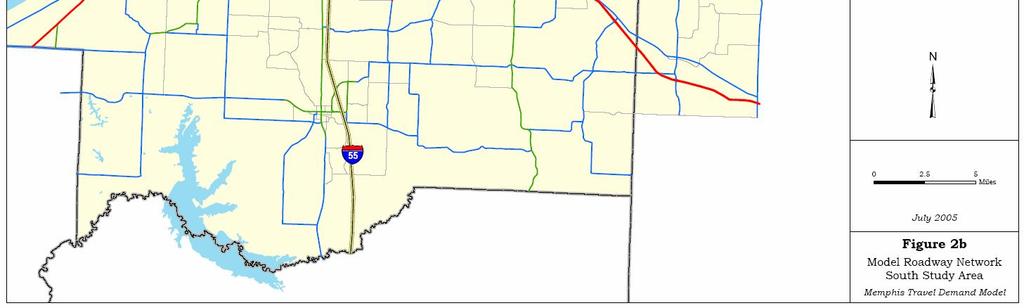
9 APPENDIX G - TRAVEL DEMAND MODEL DOCUMENTATION 7.0 YEAR 2025 AND2040 E+C MODEL RESULTS After incorporating the changes into the TDM, two model runs were conducted to identify the deficiencies of the E+C network at year 2025 (the year for high priority LRTP projects) and 2040 (the year for low priority LRTP projects). For year 2025 model results, the Vehicle Miles of Travel (VMT) is summarized by roadway functional classification and compared with the base year 2004 results in Table 10. Assigned traffic volumes across screenlines and cutlines are also compared with the base year 2004 results in Table 11. Figure 1 shows the screenline and cutline locations. A roadway Level of Service (LOS) map for the E+C network is presented in Figure 2. Table 10 - Year 2025 VMT by Functional Classification Functional Classification 2004 VMT 2025 Model VMT % Difference Freeways 8,781,000 13,371,500 52% Principal Arterials 8,420,700 12,318,500 46% Minor Arterials 7,124,900 9,790,200 37% Collectors 2,653,000 4,709,000 77% Total 26,980,700 40,189,200 49% Table 11 - Year 2025 Screenline/Cutline Volume Screen Line /Cut Line 2004 Count Total 2025 Model Volume # of Counts % Difference Screenline 1 276, , % Screenline 2 764, , % Screenline 3 805, , % Cutline 1 1,306,195 1,615, % Cutline 2 162, , % Cutline 3 72, , % Cutline 4 74, , % Cutline 5 31,680 43, % G-8

10 APPENDIX G - TRAVEL DEMAND MODEL DOCUMENTATION Figure 1 - Screenline/Cutline Locations G-9

11 APPENDIX G - TRAVEL DEMAND MODEL DOCUMENTATION Figure 2 - Level of Service for Year 2025 on E+C Network G-10

12 APPENDIX G - TRAVEL DEMAND MODEL DOCUMENTATION For year 2040 model results, the Vehicle Miles of Travel (VMT) is summarized by roadway functional classification and compared with the base year 2004 results in Table 12. Assigned traffic volumes across screenlines and cutlines are also compared with the base year 2004 results in Table 13. A roadway Level of Service (LOS) map for the E+C network is presented in Figure 3. Table 12 - Year 2040 VMT by Functional Classification Functional Classification 2004 VMT 2040 Model VMT % Difference Freeways 8,781,000 15,515,100 77% Principal Arterials 8,420,700 15,433,400 83% Minor Arterials 7,124,900 12,411,100 74% Collectors 2,653,000 7,108, % Total 26,980,700 50,468,300 87% Table 13 - Year 2040 Screenline/Cutline Volume Screen Line /Cut Line 2004 Count Total 2040 Model Volume # of Counts % Difference Screenline 1 276, , % Screenline 2 764,201 1,211, % Screenline 3 805,834 1,099, % Cutline 1 1,306,195 1,794, % Cutline 2 162, , % Cutline 3 72, , % Cutline 4 74, , % Cutline 5 31,680 54, % G-11

13 APPENDIX G - TRAVEL DEMAND MODEL DOCUMENTATION Figure 3 - Level of Service for Year 2040 on E+C Network G-12

14 Technical Memoranda 1a Network and TAZ Development 1b Travel Time Studies 2 Regional Economic and Demographic Forecasts Methodology and Results 3 Trip Generation 4 Destination Choice 5 Time-of-Day Model 6 Mode Choice 7 Freight Model 8a Highway Assignment, Transit Assignment, and Feedback Procedures 8b Link Capacity Development 9 Highway Validation Procedures and Goals and Transit Assignment Reasonableness Checking Procedures 10 Base and Future Year Signalized Intersection Tools and Future Year Signal Location Forecasting Methodology 11 Model Calibration and Assignment Validation Results 12 Future Year Model Development and Results 1 G - 13

15 Technical Memorandum #1 (a) Network and TAZ Development This memorandum details the network and transportation analysis zone (TAZ) development for the Memphis Travel Demand Model Update. It includes revisions that were completed between January and July These revisions include functional classification coding, transit route coding, traffic count location coding, screenline/cutline coding, walk access link coding, supplemental centroid connector coding, future year road identification, and network quality review. It also includes future year highway and transit network coding and revisions completed in Contents Network Development Methodology - Overview - Identification of Network Roads - Identification of Transit Routes - Network Corrections - Collection of Network Attributes - Network Data Population - Centroid Connectors - Centerline-Mile Summary - Screenline and Cutline Development - Traffic Counts and Transit Boardings - Corridor Travel Time Study - Federal Functional Classification - Supplemental Traffic Count Request - Corridor Travel Time Analysis - Area Type - Capacity Equation Application Refinement of Traffic Analysis Zone Structure - Overview - TAZ Refinement Criteria - Special Generators - Process Appendix A Base Year (2004) Transit Route Attributes Appendix B Final TAZ Geographic Boundaries 1 G - 14

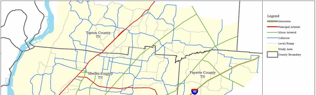
16 Network Development Methodology Development of the highway network involved identifying the network roads to be included, developing the TransCAD line network, collecting network attributes, and populating network data in TransCAD. Overview In order to simulate travel within the Memphis area, a computer network must be developed that represents the street system to be modeled. The network will be represented for the entire study area, which has been expanded from the previous model for the 2004 base year update, as shown in Figure 1. The network developed for the Memphis area includes all interstates, freeways, and arterials, as well as significant collector and local roads in terms of high traffic volumes, necessary connectivity, or accommodating transit routes and walk connections for the transit model. The study area for the Memphis MPO model (Figure 1) includes all of Shelby County and portions of Tipton and Fayette Counties in Tennessee, along with all of DeSoto County and a small portion of Marshall County in Mississippi. The Memphis model study area encompasses an area of approximately 1,825 square miles, with 1,260 square miles in Tennessee and 565 square miles in Mississippi. As part of the network development, approximately 2,400 miles of roadway were identified for inclusion in the 2004 base year model. The highway network database contains attributes for each link in the line layer in TransCAD. This layer contains all of the necessary attributes for proper modeling of each of the roadways in the model, including roadway speeds and capacities. This information was collected directly or derived from field visits and available data from the Tennessee Department of Transportation. 2 G - 15

17 Figure 1. Study Area Graphic 3 G - 16

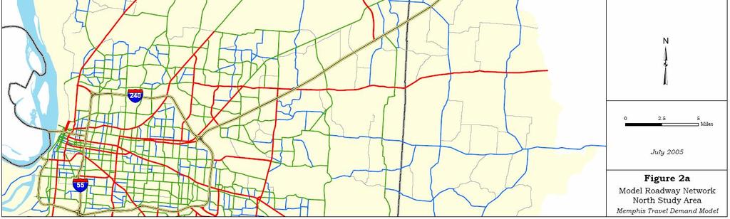
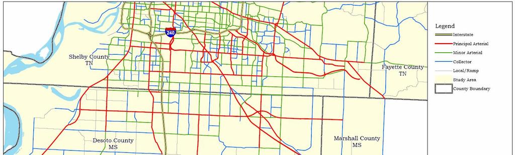
18 Identification of Network Roads The initial Memphis model network for the previous study area (shown in yellow in Figure 1) was provided by the MPO in TransCAD format. The initial network was expanded by the Kimley-Horn team to the final study area boundary outlined in red in Figure 1 using street data from TransCAD and ArcGIS. The network includes all roads of regional significance, including all interstates, freeways, and arterials within the MPO area. The model also includes collectors and local roads that have heavy traffic volumes, provide connectivity, or to accommodate transit routes and walk access/egress, or have plans for future upgrades or connections. The model network has been compared with the current Major Road and current Collector Street plans to verify that no roads were omitted in error. Figure 2 displays the Road Network identified for Memphis. In addition to using the network to model auto and truck activities, the network also serves as a base to underlay the transit route system. In TransCAD, transit routes are not maintained as separate database files. Instead, a transit route (such as a bus route) is represented by identifying the highway links used by the bus route. Consequently, many local roads in the urban area were added into the highway network to represent local roads used by buses to entire neighborhoods. The base year transit route system includes bus routes (for both regular and express fixed route buses) and trolley routes. Specifically with the trolley, there are trolley right-of-ways that are not accessible by auto. Therefore, additional right-of-way lines were also added. See Appendix A for base year transit route attributes. The transit route system was coded with walk access/egress and walk transfers. The route system also allows drive access at four park-and-ride lots for base year: North End Terminal, Central Station, Cleveland Station, and American Way Transit Center. Access connections from the highway network to the park-and-ride lots were also added. Identification of Transit Routes The route system was coded based on MATA hardcopy schedules published in June Each route was coded as having two travel directions: inbound toward the North End Terminal, and outbound away from the North End Terminal. Routes which do not serve North End Terminal were generally coded as outbound: west to east, or outbound: south to north. Vehicle headway was coded for 4 time periods: AM peak, midday, PM peak, and night. The headway data was also taken from the printed schedules. 4 G - 17

19 The base year route system has two distinct modes: trolley and bus. Express bus was not modeled as distinct mode in the model because there is no sufficient data to calibrate a separate mode choice model for express bus only. However, the model allows express bus to utilize its distinct fares. This is done by using a separate express bus fare matrix and specifying this fare matrix index in the route attributes table. Light rail is an additional distinct mode for future year. Network Corrections As a part of the network development process, corrections and quality checks were made to the TransCAD network. Corrections made to the Memphis network include the following: Verified roadway alignments and termini The network was cleaned to aerial photography, especially in Mississippi, where some roads were consistently misaligned, primarily a function of merging data from the two states with different projection systems. The Kimley-Horn team also verified necessary modifications to roadway links to provide for representative conditions. Repaired fragmented roadway links Many links (roadway sections between intersection nodes) consisted of multiple individual fragments. This increases the likelihood of disconnected roadways, which increases file size and causes traffic assignment problems. Using TransCAD s map editing tools, the Kimley-Horn team combined fragmented roadway segments into continuous links between intersection nodes. Modified disconnected intersection nodes Some nodes in the centerline mapping were not properly aligned at as-built intersections. Using TransCAD s map editing tools, the Kimley-Horn team reviewed and properly connected intersecting roadways. 5 G - 18

20 G - 19

21 G - 20

22 Collection of Network Attributes The Memphis model requires several important attributes for each highway link, which are used in various steps throughout the model. The primary attributes required for modeling include facility type, posted speed, and attributes needed for capacity development. The attributes recorded during the data collection effort included: Posted Speed Limit Area Type (CBD, Urban, Rural, Suburban) Driveways (None, Low Density, Medium Density, High Density) Median Treatment (No Median, Divided, Two-Way Left Turn Lanes) Roadway Functional Classification (Interstate, Other Freeway, Principal (Major) Arterial, Minor Arterial, Collector, Local) Heavy Vehicle Restriction Through Lanes per Direction Average Lane Width by Direction Average Shoulder Width by Direction Parking Comments The data collection of network attributes came from two sources: 1) Tennessee DOT Tennessee Roadway Information Management System (TRIMS) photography data and 2) field assessments. The TRIMS photography data was collected in 2003 by Mandli Communications, Inc. and included a snapshot of the cross section and the side of the road every 50 feet along each corridor. Software provided by the vendor allows users to view the photographs for each corridor in succession as if they were moving down the road. An example set of photographs are shown in Figure 3. This data was provided for all of the major roads in Tennessee included in the study area. Roads that were not included in this database were field reviewed by the consultant to collect the necessary data in fall of G - 21

23 Figure 3. Sample TRIMS Photography Data Front View Side View Network Data Population A TransCAD data entry form was developed as part of the Network development to facilitate data entry directly into the TransCAD network. Using the tool, data was entered into the network either while traveling in the field or in the office while viewing the photography data. Using this tool eliminated the need for paper forms and subsequent data entry, and streamlined the process by using pull-down menus. The tool also allowed for copying and pasting of data from link to link, which also increased data entry efficiency. Figure 4 shows the toolbar for the data collection tool, while Figure 5 shows the form used to enter the data for each link. Figure 4. Memphis Data Collection Toolbar 9 G - 22

24 Figure 5. Memphis Link Data Entry Form Centroid Connectors Centroid connectors were developed using the TransCAD automated connector placement process. This created a set of centroid connectors which can be readily used to do network skimming. The automated TransCAD process is able to be applied in one of two ways. It can either draw one or more centroid connectors to the closest line layer nodes; or it can be applied to draw a single centroid connector by breaking the closest line and inserting a node which is then used to accept the centroid connector. When TransCAD is used to draw connections to the closest node, most of the connections are made at intersections. Attaching centroid connectors to line segments 10 G - 23

25 is more desirable because the connectors could be used to represent local road loading points. Consequently, TransCAD was used to develop the centroid connectors by placing a single connector to the closest line layer segment. It is not desirable to have centroid connects attached to interstate, freeway, ramp, or expressway facilities. Therefore, prior to using the TransCAD process, a selection set of roads eligible to receive a centroid connector was made. When TransCAD s automated process was used, the centroid point ID was made to be identical to the node ID in the line layer network. This provides consistency in later modeling steps when trip tables are assigned to the line layer network. The first generation of the line layer (highway network) was completed by placing one centroid connector per zone. Where appropriate, additional connectors have been added manually to provide multiple connections per zone. In addition, automated connectors were moved when the connectors were placed inappropriately after reviewing access, local road network, and development density. Within the CBD and most of the urban zones, additional walking connectors were developed. These connectors enhanced transit accessibility and serve to represent cross block pedestrian movements which cannot be accommodated by the highway centroid connectors. Centerline-Mile Summary Part of the development process was the addition of the functional classification codes to the network links. These codes, developed by the Federal Highway Administration (FHWA) and implemented by the Tennessee and Mississippi Departments of Transportation, categorize all of the roads in the FHWA system into various functional classifications. The classifications are based on such factors as road cross-section, traffic volume, access control, and traffic served. Functional classification codes were added for all links in the network. The FHWA codes will be used in addition to the Memphis Major Road Plan as a basis for developing capacities in the Memphis model. They also will be used to calibrate and validate the model, since calibration targets and allowable volume differences vary by facility type. A summary of centerline-miles by FHWA functional classification code for the existing network is shown in Table G - 24

26 Table 1. Memphis Centerline-Miles Summary by Functional Class FHWA Functional Class Description Code Centerline Miles Rural Interstate 1 26 Rural Principal (Major) Arterial 2 71 Rural Freeway Ramp 3 6 Rural Minor Arterial 6 98 Rural Major Collector Rural Minor Collector Rural Local Access Urban Interstate Urban Freeway/ Expressways Urban Freeway Ramp Urban Principal (Major) Arterial Urban Minor Arterial Urban Collector Urban Local Access Total Rural Roads 1,077 Total Urban Roads 1,322 Total All Roads 2,399 Screenline and Cutline Development Several screenlines and cutlines were developed for the Memphis model to help determine the accuracy of traffic assignment, especially with regards to regional flow. Screenlines and cutlines were developed that bisect the study area crossing only road locations that have the most available traffic counts. Typically, screenlines follow natural boundaries and barriers, such as rivers, streams, railroad tracks, and access controlled facilities, as deemed appropriate. Cutlines are applied with less rigorous standards, and have been used to capture movements in particular corridors. The location and number of screenlines and cutlines were coordinated with the MPO. Based on these screenline locations, supplemental traffic counts are being requested to provide traffic counts at screenline/cutline crossing where no count is available. Figure 6 shows the locations of the screenlines and cutlines. In the TransCAD network, these screenlines and cutlines have been entered numerically into an attribute field titled Screenline. During the model calibration and validation process, these locations will be used to provide screenline and cutline performance. 12 G - 25

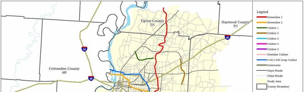
27 G - 26

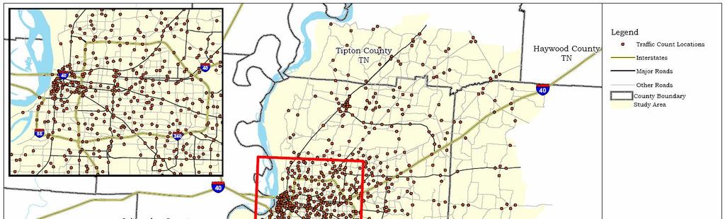
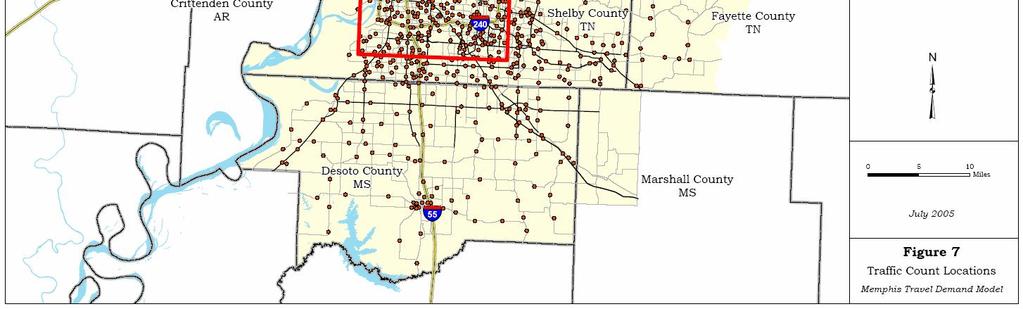
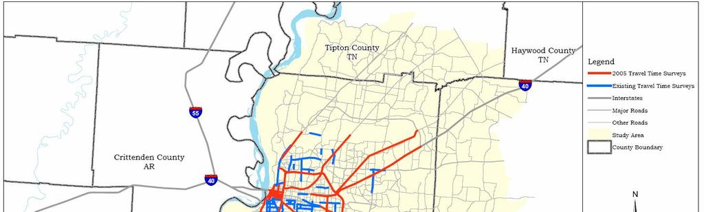
28 Traffic Counts and Transit Boardings As specified in the study design, AM peak period, PM peak period, midday off-peak, and night off-peak periods, daily traffic counts, and commercial vehicle count data will be needed throughout the model network for model calibration and validation. The Kimley-Horn team has processed and homogenized this information, bringing some counts from electronic format and some counts in hard copy format into the same format. These count locations have been coded into the TransCAD network for final determination of screenline/cutline location and supplemental traffic count requests. Figure 7 shows the traffic count locations that were coded into the TransCAD network. Traffic counts are currently being appended to the TransCAD network at these locations. Fields that will be included in the traffic count data include: o 2000_ADT o 2004_ADT o 2004_AM (AM Peak Period) o 2004_Midday (Midday Off-Peak Period) o 2004_PM (PM Peak Period) o 2004_Night (Night Off-Peak Period) o 2004_Auto (Daily Automobiles) o 2004_SU (Daily Single-Unit Trucks) o 2004_CU (Daily Combination-Unit Trucks) In addition, transit ridership data (boardings) were obtained from MATA. The transit boardings were aggregated by three levels: MATA transit line, Route sub-group, and Route group. These boarding counts were coded into the transit route table and the base year transit assignment results were compared with the observed boarding in all three different levels. In addition, two screenlines were developed and provided by MATA, and were used during the transit assignment validation. Corridor Travel Time Study During a previous contract with the City of Memphis, Kimley-Horn conducted peak period travel time runs along signalized major and minor arterials throughout Shelby County. Additional travel time runs were taken by the Kimley-Horn team in 2005 in urban and rural Desoto County, in Shelby County along collectors and freeways, and along facilities extending into Fayette County. These travel time runs were conducted using the average floating vehicle method during the AM and PM peak periods in both travel directions. Available loaded speed data by peak period will be input for each link based on this information. Figure 8 shows the locations of the travel time study corridors and 2003 travel time study data is also available from the MPO, but it 14 G - 27

29 is currently not in GIS format. Travel time data from 1999 would need to be reviewed for applicability (due to potential changes in corridor cross-sections, volumes, and signal density) before inclusion in the model update. 15 G - 28

30 G - 29

31 G - 30

32 Federal Functional Classification Federal functional classification refers to the federal designation (e.g., freeway, ramp, or principal arterial) needed for performing conformity analysis, capacity analysis, and quantifying the percentage of lane miles by functional class. These functional classes have been coded into the TransCAD network for modeling purposes. Figure 2 shows the coded functional classification link data. As specified in the study design, the consultant team will work with the Steering Committee to develop a corresponding relationship between FHWA functional classifications and functional class as it pertains to the Major Road Plan. Since the Memphis MPO and surrounding agencies reference the Major Road Plan when identifying functional class, efforts will be made to make sure that the Major Road Plan functional class designation is maintained in the roadway network database. Upcoming Steps The model network will be enhanced with additional information as it is collected, developed, or made available. The list below details data that are planned to be added to the Memphis network in the upcoming three months. Supplemental Traffic Count Request The Kimley-Horn team will map out the count coverage and assess the quality of count data (e.g., time periods and accuracy). This process will identify holes in the count coverage. The Kimley-Horn team will coordinate with the Steering Committee to develop plans to obtain additional traffic counts from state, county, and local agencies. It is projected that up to 75 additional bi-directional hourly traffic counts (conducted over a continuous 24-hour period) may be needed throughout the study area. The required number of traffic counts can be determined after coordinating with the Steering Committee to ascertain the accuracy of their available data and their ability to commit resources to obtain remaining data needs. Corridor Travel Time Analysis As specified in the Memphis Study Design, the skim matrices will be determined based on travel impedance (i.e., speed or travel time). During the peak periods, the travel impedance should not necessarily be a free-flow speed, but rather a more representative loaded speed or congested speed. Results from the travel time runs will be used during the model development and calibration process to assist in validation that the travel demand model is effectively representing the effect that traffic volumes have on travel speed, and that the proper volume-delay curves are being used. 18 G - 31

33 Area Type This identifies the type of area (e.g., urban or rural) and is used in customizing link capacities. While the field data collection effort identified a preliminary area type, the consultant team and the Steering Committee will define an area type categorization scheme that incorporates population and employment densities as variables to categorize districts. The advantage of an automated method to determine area type is that future year area types can be determined using the same methodology. Area types will be applied to links using GIS after the methodology is established. Capacity Equation Application Daily and hourly capacities will be developed for the Memphis model. This will allow collected street data to provide the most accurate representation of actual capacity (levels of service A through E) on an individual link. These capacities are implemented using an equation that takes into account data such as facility type, speed limit, lanes, median treatment, area type, average land width, and average shoulder width. The capacity equations are built into the model process, so modifications to network attributes automatically update the capacity in subsequent runs. Refinement of Traffic Analysis Zone Structure Overview As a part of the Memphis MPO regional travel demand model update, it was expressed early in the process that the existing traffic analysis zone (TAZ) structure needed to be expanded and refined. The geographic expansion included TAZ coverage for all of DeSoto County and the northwest quadrant of Marshall County located in Mississippi, the southern portion of Tipton County, Tennessee, and the western portion of Fayette County, Tennessee. Refinement of the TAZ structure within Shelby County and the City of Memphis was also identified as part of the update so that new developments, higher land use density, and other socioeconomic variables could be best represented during the eventual traffic assignment phase of model development. The TAZ development process was comprehensive and iterative as it involved the establishment of guidelines or criteria, input from the Peer Review Committee, and local input from the MPO Steering Committee. This iterative approach allowed for the application of technical knowledge and experience associated with TAZ structure development as well as local knowledge for refinement and its influence on the final structure of the TAZs to serve the regional model. The expanded and refined TAZ structure now consists of 1,237 internal zones and covers approximately 1,825 square 19 G - 32

34 miles. This is approximately one zone per 1.47 square land miles, a relatively dense zonal structure for a metropolitan area such as the Memphis MPO. TAZ Refinement Criteria In developing and refining the traffic analysis zone (TAZ) structure for the Memphis MPO regional travel demand model, several guidelines and criteria were established as a basis for development. For example, zones were developed that are homogenous with respect to land use and socioeconomic data. Whenever possible, zone boundaries followed physical and natural geographic features. Finally, census tract, census block group, and even census block geography boundaries were followed to the extent possible to allow for easy access to census data. Traffic analysis zone development and modification was influenced by the following criteria: Geographic features Transportation facilities TAZ boundary configuration consistent with census tract boundaries, census block groups in rural/suburban areas, and census blocks in the CBD In more densely populated areas (e.g., CBD), additional TAZs will match census block group boundaries or census block boundaries where appropriate Ensure population and employment density is consistent across the zone (avoid a disproportionate pocket of population or employment within zones) Ensure land uses are consistent across the zone Evaluation of existing land uses and zoning Cross reference with an evaluation of the future land use plan Configuration will be consistent with the available transportation network/infrastructure serving the zone Configure zones and zonal boundaries such that trips can be loaded appropriately (meaning that we will load the proper roadway functional classification) to the internal transportation network within the TAZ itself. In the development of the Memphis MPO TAZ structure, these criteria or guidelines were followed to the extent possible but not without some variation. Several locations in outlying rural areas have TAZs that are split into smaller geographic areas than the provided Census Block boundaries. There were also locations where the shape or configuration of the TAZ was illogical in relation to roadway network access or land development. In such cases these zones were either split or combined with adjacent zones to provide a more desirable zone structure. Additionally, throughout the process TAZ boundary locations were evaluated relative to infrastructure, right-of-way, geographic features, identified special generators, land 20 G - 33

35 uses and future land use planning. Socio-economic data by census tract and census block group (where applicable) along with existing land use and future land use maps, model network area coverage, and necessary regional aerial photography were all used in determining the need for splitting, realigning, or adding additional TAZs. Special Generators As a part of the TAZ development special generators had to be accounted for within the regional travel demand model. Special generators were identified and singled out because the socio-economic data associated with these TAZs cannot truly reflect the traffic volume activity going on at these locations. Such special generators typically include industrial parks, universities, major employers, and regional and local shopping centers. Special generators for the Memphis MPO regional model include the following: Memphis International Airport FedEx Operations at Memphis International Airport Graceland Process The process began using the existing TAZ structure from the previous regional model for the MPO and identifying additional zonal needs beyond Shelby County and portions of Fayette and DeSoto Counties. As defined in the study design process, this included all of DeSoto County, the northwest portion of Marshall County, the southern part of Tipton County, and the entire western portion of Fayette County bordering Shelby County. The initial expansion of the TAZ coverage was based on Census Tract boundaries in these outlying areas. This was quickly identified as insufficient as the TAZs were very large when relying solely on the Census Tract boundary layer. At the tract level in these areas much of the newer development and intent of the future land use plan would have been under represented in interim and future traffic assignments. Following this initial assessment it was decided that census block boundaries would prove more effective in establishing TAZ boundaries. At the census block layer smaller areas of development and growth could be captured. The refinement of TAZs in the suburban and rural areas of the model was carried over as it resulted in zones matching up well with network coverage in outlying areas and avoided large zones loading at only a few select points in the roadway network. For Shelby County and the City of Memphis, the old TAZ structure provided the initial backdrop. Much of the old TAZ structure was based on a combination of census tract, census block group, and in some cases census block boundaries. However, for refinement of the TAZ structure it was determined necessary that census block 21 G - 34

36 boundaries be used for all of Shelby County and particularly in the Memphis CBD. This approach resulted in the extensive refinement of the TAZ structure for Shelby County and the City of Memphis. Only in certain cases was there deviation from the use of census origin boundaries. The focus was to limit disaggregation efforts that involved splitting or reallocating census data from census tracts, census block groups, or census block data source configurations and to modified TAZs. Only in select instances (future planned roadways, new planned developments, current large blocks with very inconsistent internal land uses, or known future high activity centers) were such variations from the criteria practiced. Typically, such cases were the direct result of local knowledge input and review of the proposed TAZ structure. The TAZ structure was then reviewed by the MPO Steering Committee. Where appropriate, comments from the Steering Committee were applied and incorporated into the final TAZ structure. Once consensus on the TAZ structure and TAZ density was achieved it was forwarded to other members of the Memphis MPO regional model development team for review. Other team members were then responsible for identifying and coding necessary trip generation variable data (population, households, auto ownership, employment, etc.) from employment and census data resources into the TAZ database. Additionally, with the completion of the TAZ structure and the regional model network, centroid connectors for each TAZ were then coded into the regional model network. A map showing the new TAZ boundaries with other geographic features is included as Appendix B. 22 G - 35

37 Appendix A Base Year (2004) Transit Route Attributes FareMatrix AM_Dwell MD_Dwell PM_Dwell OP_Dwell Route_Name RETIREYEAR LineName Mode Index AM_Headway MD_Headway PM_Headway OP_Headway Time Time Time Time 2A Medical Center[2A,2C] A_R Medical Center[2A,2C] C Medical Center[2A,2C] C_R Medical Center[2A,2C] L Lauderdale [2L,2W] L_R Lauderdale [2L,2W] W Lauderdale [2L,2W] W_R Lauderdale [2L,2W] A Walker [4A,4C] A_R Walker [4A,4C] C Walker [4A,4C] C_R Walker [4A,4C] Air Park[7A, 7B] _R Air Park[7A, 7B] Chelsea [8] _R Chelsea [8] S Lamar [10C,10S] S_R Lamar [10C,10S] C Lamar [10C,10S] C_R Lamar [10C,10S] RG Watkins[10RG,10RL] RG_R Watkins[10RG,10RL] RL Watkins[10RG,10RL] RL_R Watkins[10RG,10RL] C Thomas[11F,11C] C_R Thomas[11F,11C] F Thomas[11F,11C] F_R Thomas[11F,11C] S Tulane/Hodge[11T,11S] S_R Tulane/Hodge[11T,11S] T Tulane/Hodge[11T,11S] T_R Tulane/Hodge[11T,11S] Presidents Island [15] _R Presidents Island [15] M Vollintine[19RA,19NA,19M] M_R Vollintine[19RA,19NA,19M] NA Vollintine[19RA,19NA,19M] NA_R Vollintine[19RA,19NA,19M] R Third [19W, 19R] G - 36

38 FareMatrix AM_Dwell MD_Dwell PM_Dwell OP_Dwell Route_Name RETIREYEAR LineName Mode Index AM_Headway MD_Headway PM_Headway OP_Headway Time Time Time Time 19R_R Third [19W, 19R] RA Vollintine[19RA,19NA,19M] RA_R Vollintine[19RA,19NA,19M] W Third [19W, 19R] W_R Third [19W, 19R] Bellevue/Winchester [20] _R Bellevue/Winchester [20] L Poplar [22] L_R Poplar [22] Perkins [30] _R Perkins [30] Crosstown [31] _R Crosstown [31] A E Parkway[32A,32F,32N] A_R E Parkway[32A,32F,32N] F E Parkway[32A,32F,32N] F_R E Parkway[32A,32F,32N] N E Parkway[32A,32F,32N] N_R E Parkway[32A,32F,32N] Highland[33] _R Highland[33] B Union/WalnutG[34R,34B] B_R Union/WalnutG[34R,34B] M McLemore [34M,34N] M_R McLemore [34M,34N] N McLemore [34M,34N] N_R McLemore [34M,34N] R Union/WalnutG[34R,34B] R_R Union/WalnutG[34R,34B] Southgate [35] _R Southgate [35] Raleigh[40,40B] _R Raleigh[40,40B] B Raleigh[40,40B] B_R Raleigh[40,40B] Collierville[41] _R Collierville[41] B ElvisPresley [43B,43H,43S] B_R ElvisPresley [43B,43H,43S] H ElvisPresley [43B,43H,43S] H_R ElvisPresley [43B,43H,43S] S ElvisPresley [43B,43H,43S] G - 37

39 FareMatrix AM_Dwell MD_Dwell PM_Dwell OP_Dwell Route_Name RETIREYEAR LineName Mode Index AM_Headway MD_Headway PM_Headway OP_Headway Time Time Time Time 43S_R ElvisPresley [43B,43H,43S] G Poplar[50G,50W,50Y] G_R Poplar[50G,50W,50Y] W Poplar[50G,50W,50Y] W_R Poplar[50G,50W,50Y] Y Poplar[50G,50W,50Y] Y_R Poplar[50G,50W,50Y] B Park[52Q,52B,52SF] B_R Park[52Q,52B,52SF] M Jackson[52M,52R,52SE] M_R Jackson[52M,52R,52SE] Q Park[52Q,52B,52SF] Q_R Park[52Q,52B,52SF] R Jackson[52M,52R,52SE] R_R Jackson[52M,52R,52SE] SE Jackson[52M,52R,52SE] SE_R Jackson[52M,52R,52SE] SF Park[52Q,52B,52SF] SF_R Park[52Q,52B,52SF] B Summer[53B,53S] B_R Summer[53B,53S] I Florida [53I,53L,53W] I_R Florida [53I,53L,53W] L Florida [53I,53L,53W] L_R Florida [53I,53L,53W] S Summer[53B,53S] S_R Summer[53B,53S] W Florida [53I,53L,53W] W_R Florida [53I,53L,53W] Union [56] _R Union [56] B FoxMeadowsB[58B] B_R FoxMeadowsB[58B] G Frayser/EMemphis[62G,62W] G_R Frayser/EMemphis[62G,62W] W Frayser/EMemphis[62G,62W] W_R Frayser/EMemphis[62G,62W] Winchester[69] _R Winchester[69] Cordova [80] _R Cordova [80] B Cordova [80] G - 38

40 FareMatrix AM_Dwell MD_Dwell PM_Dwell OP_Dwell Route_Name RETIREYEAR LineName Mode Index AM_Headway MD_Headway PM_Headway OP_Headway Time Time Time Time 80B_R Cordova [80] ShelbyDr/HickoryHill [81] _R ShelbyDr/HickoryHill [81] GermantownPkwy[82] _R GermantownPkwy[82] WalkerHomes/Westwood _R WalkerHomes/Westwood Neely/Shelby Dr _R Neely/Shelby Dr HickoryHill/Winchester[93] _R HickoryHill/Winchester[93] Trolley Madison St IB 9999 Madison St Trolley Trolley Madison St OB 9999 Madison St Trolley Trolley Main St NB 9999 Main St Trolley Trolley Main St SB 9999 Main St Trolley Trolley Riverfront Loop 9999 Riverfront Trolley G - 39

41 Appendix B Final TAZ Geographic Boundaries 27 G - 40

42 Technical Memorandum #1b Travel Time Studies This memorandum details the development of the Travel Time adjustment factors for the Memphis Travel Demand Model Update. Contents Methodology - Overview - Determination of Travel Time Study Corridors - Travel Time Study Appendix A Summary of Travel Time Runs Methodology Development of the travel time factors for the Memphis MPO Model included identifying study corridors, administering a travel time survey, analyzing the survey data to develop speed adjustment factors by area type, roadway facility type, posted speeds, and time-of-day. These factors were used to develop free-flow speeds and congested speeds for use in the Memphis model. Overview Travel time is defined as the total time for a vehicle to complete a designated trip over a section of road or from a specified origin to a specified destination. A travel time study provides valuable information about the delay associated with the study corridor, including congestion delay and intersection delay. Traditionally, free flow speeds have been used for trip distribution procedures in travel demand models. In the absence of observed speed measurements, posted speeds have often been used as a surrogate to estimate free flow speeds. However, during peak periods, when many trips are made, the travel impedance is not necessarily free flow speed, but rather a more representative loaded speed or congested speed. Correspondingly, often during non-peak periods or in the non-peak direction of travel, the motorists are observed traveling in excess of the posted speed limit. 1 G - 41

43 For the development of the Memphis Travel Demand Model (TDM), posted speeds for each link in the network were collected as a part of the network data collection process. Subsequent to this, travel time studies were conducted along selected corridors to estimate congested speeds on to develop system-wide congested speeds that will be compared to model congested speeds. Results from the travel time runs are being used during the model development for the trip distribution, mode choice, and highway/transit assignment submodels. They have been used to develop free-flow speed adjustment factors and to estimate congested speeds for each time period. Determination of Travel Time Study Corridors The emphasis of the study was mainly on the freeways and arterials not on collector or local streets. Corridors were selected based on their functional classification, significance, geographic location, posted speeds, and length. Travel time data was collected on approximately 20% (390 miles) of the total freeway lane miles and 10% (910 miles) of the arterial streets included in the model network. Travel time studies were conducted on a total of 177 miles of roadway network. Table 1 shows the description of each travel time corridor. Figure 1 shows all the travel time study corridors. 2 G - 42

44 Table 1. Travel Time Study Corridors Route ID Route From To Functional Class Length (mi) 1 Perkins Rd Sam Cooper Blvd US 78/Lamar Ave Minor Arterial Highway 300 Highway 51 I-40 Other Freeway 1.1 I-40 Highway 300 I-240 Interstate 8.94 I-240/I-40 Loop to Highway 300 Interstate Sam Cooper Blvd I-40 Sam Cooper Blvd Holmes St I-40 Other Freeway 3.99 Paul Barrett Pkwy Overpass Interstate Highway 70 I-40 Underpass Paul Barrett Pkwy Overpass Major Arterial Jackson Ave Bellevue Blvd I-40 Major Arterial 6.42 Austin Peay Pkwy I-40 Loosahatchie Pkwy Major Arterial Poplar Ave Goodlett Street Kirby Pkwy Major Arterial Bill Morris Parkway Lamar Ave /US 78 Elvis Presley Boulevard I-240 Highway 72 Other Freeway I-240 Downtown (West Side of Loop) Goodman Rd Major Arterial Goodman Road Brooks Rd Major Arterial Highway 61 I-55 State Line Rd Major Arterial 7.31 State Line Road I-55 North Highway 61 I-55 Minor Arterial 7.89 I-55/I-240 Interchange Riverside Dr Interstate 5.34 Riverside Dr I-55 I-40 Minor Arterial G - 43

45 Table 1. Travel Time Study Corridors (cont.) Route ID 11 Route From To I-40 Downtown West of I- 40/Riverside Interchange Functional Class Length (mi) I-240 Interstate 1.44 Union Ave Riverside Dr I-240 Downtown Major Arterial Madison Ave I-240 Downtown Front Street Minor Arterial 2.42 Jefferson Ave Front St I-240 Downtown Minor Arterial 1.79 Poplar Ave I-240 Downtown Front Street Major Arterial nd St G.E. Patterson St Chelsea Avenue Minor Arterial rd St Chelsea Ave G.E. Patterson St Minor Arterial 2.9 Manassas St Chelsea Ave Union Ave Minor Arterial 1.86 Walnut St Union Ave Linden Ave Local Highway 51 Millington Rd (South Intersection) Fite Rd Major Arterial G - 44

46 G - 45

47 Travel Time Study The most common method used to conduct travel time surveys is performing floating car runs. This method was employed for the Memphis TDM. The driver of the vehicle was instructed to maintain the profile of an average car in the traffic stream according to his or her best judgment of the traffic stream s speed. A GPS unit was used to continuously log travel time information directly to TransCAD. The position of the GPS receiver is automatically recorded to a geographic layer at predefined time intervals (2 seconds for this study). TransCAD stores the data in a standard format geographic file (which is native to TransCAD) as a series of points. This is a relatively simple and cost-effective procedure in which a single person with a GPS unit hooked to a laptop with TransCAD software can collect travel time data on study corridors. Travel Time Survey Data Processing The travel time runs were conducted during February and March The field data collected is stored in TransCAD s native standard geographic file format (.dbd). The data was exported to spreadsheets to enable further analysis. The distances between points along the corridor between two major cross streets were summed to determine the total distance between the cross streets and then converted to miles. The travel time was then determined based on the difference in time from one major cross street to another and the distance between them. The average travel time was then compared to the posted speed for each of these roadway segments and adjustment factors were developed. These factors were summarized based on roadway facility type, area type, posted speed, and time-of-day. Roadway functional classes 1, 11, and 12 were grouped to form the Freeways; functional classes 2, 6, 14, and 16 were grouped to form the arterials; and classes 7, 8, 9, 17, and 19 were grouped to form the collectors/locals. A description of the functional classifications can be found in the Network and TAZ Development Memo Technical Memorandum #1(a). Arterials were sub-divided into two speed categories based on their posted speeds: greater than or equal to 45 mph and less than 45 mph. No significant advantage was found to performing such an exercise for the Freeway and collector/local. The Memphis TDM uses four time-of-day periods. These are the AM peak period (6 AM 9 AM), midday off-peak period (9 AM 2 PM), PM peak period (2 PM - 6 PM), and night off-peak period (6 PM 6 AM). Time-of-Day Memo Technical Memorandum #5 contains a detailed discussion of the determination of these time periods. 6 G - 46

48 The travel time surveys were conducted for the AM, midday, and PM periods. Data was not collected for the night period. Factors have been developed for comparison and calibration purposes for AM, midday, and PM time periods. Night time congested speeds will not be evaluated. Table 2 shows the free-flow speed adjustment factors used to estimate free-flow travel times in the Memphis Model. These factors, which are primarily based on the Midday time period, are applied to the posted speed to estimate free-flow speeds used for trip assignment. For example, if an arterial has posted speed of 40 mph, and is located in the urban area, then a factor of 0.85 (from table 2) is applied to its posted speed to calculate its free-flow speed (40 *0.85 = 34 mph). The calculated free-flow speed is then used as an input of the volume-delay function in the highway assignment procedure. Table 2. Free-Flow Speed Adjustment Factors Area Type Freeways Arterial Collector and Local All >=45 mph <45 mph All CBD Urban Suburban Rural The travel time factors were summarized for each time period by facility type, area type, and speed category. Table 3 shows the congested speed estimation factors that have been developed based on the travel time studies. These factors are used to create an estimated congested travel time, by time period, in the initial network skims for use in the initial trip distribution and mode choice submodels. For example, if an arterial has posted speed of 40 mph, and is located in the urban area, then a factor of 0.80 (from table 3) is applied to its posted speed to calculate its congested speed for AM peak period (40 *0.80 = 32 mph). The calculated congested speed is then used to calculate the initial highway travel times for this arterial. The calculated congested travel time is used as a starting cost for the highway assignment procedure, in order to achieve faster convergence of the equilibrium assignment procedure. As part of the model calibration process, a table similar to Table 3 will be created for model results to confirm that the travel demand model is effectively representing the 7 G - 47

49 effect that traffic volumes have on travel speed, and that the proper capacities and volume-delay curves are being used. Table 3. Congested Speed Estimation Factors Area Type CBD Urban Suburban and Rural Suburban and Rural Time-of-Day Freeways Arterial Collector and Local All >=45 mph <45 mph All AM PM Midday Night AM PM Midday Night AM PM Midday Night AM PM Midday Night G - 48

50 Appendix A Summary of Travel Time Runs Route #1: Perkins Road Section_ID From To Distance Average Travel Speed (mph) (Mi) NB_AM NB_MD NB_PM SB_AM SB_MD SB_PM 1 Delp St. US US 78 Old Lamar Old Lamar Winchester Winchester Knight Arnold Knight Arnold American Way American Way I I240 Dunn Ave Dunn Ave. Quince Quince Park Park Southern Southern Poplar Poplar Walnut Grove Walnut Grove Sam Cooper G - 49

51 Route #2: Highway 300, I-40 and I-240 Loop Section Distance Average Travel Speed (mph) From To ID (Mi) NB/EB_AM NB/EB_MD NB/EB_PM SB/WB_AM SB/WB_MD SB/WB_PM 1 Highway 51 I-40 E/W I-40 E/W Watkins Watkins Hollywood Hollywood 5 New Allen / Warford 6 Jackson New Allen / Warford Jackson Covington Pike Covington 7 Highway Pike 8 Highway 70 Sam Cooper Walnut 9 Sam Cooper Grove 10 Walnut Grove 11 Poplar Poplar Bill Morris Pkwy Bill Morris Pkwy Mt. Moriah Mt. Moriah Perkins Perkins Getwell Getwell Lamar Lamar Airways Airways Millbranch Millbranch I I-240 Norris Norris South Parkway South Parkway Crump Crump Union G - 50

52 Route #2: Highway 300, I-40 and I-240 Loop (cont.) Section Distance Average Travel Speed (mph) From To ID (Mi) NB/EB_AM NB/EB_MD NB/EB_PM SB/WB_AM SB/WB_MD SB/WB_PM 23 Union Madison Madison I-40 N/S I-40 N/S Jackson Jackson Chelsea Chelsea I-40 E/W I-40 E/W Highway Route #3: Sam Cooper / I-40 Section Distance Average Travel Speed (mph) From To ID (Mi) EB_AM EB_OP EB_PM WB_AM WB_OP WB_PM 1 Holmes Rd. Highland Highland Graham St Graham St. Perkins Rd Perkins Rd. I-40/I I-40/I-240 Sycamore View Rd Sycamore View Rd. Whitten Rd Whitten Rd. Appling Rd Appling Rd. Germantown Pkwy Germantown Pkwy. Highway Highway 64 Canada Rd Canada Rd. Paul Barrett Pkwy/TN G - 51

53 Route #4: Highway 70 Section Distance Average Travel Speed (mph) From To ID (Mi) EB_AM EB_OP EB_PM WB_AM WB_OP WB_PM 1 I-40 Bartlett Rd Bartlett Rd. Sycamore View Sycamore View Raleigh-LaGrange Raleigh- LaGrange Elmore Elmore Alturia Alturia Kirby-Whitten Kirby-Whitten Highway Highway 64 Yale Yale Appling Appling Germantown Rd Germantown Rd. Brunswick Brunswick Canada Rd Canada Rd. Chamber's Chapel Chamber's Chapel Paul Barrett Pkwy. / G - 52

54 Route #5: Jackson Ave / Austin Peay Pkwy Section Distance Average Travel Speed (mph) From To ID (Mi) NB/EB_AM NB/EB_MD NB/EB_PM SB/WB_AM SB/WB_MD SB/WB_PM 1 Bellevue Watkins Watkins Evergreen Evergreen McLean McLean University University North Parkway North Parkway Hollywood Hollywood Warford Warford Chelsea Chelsea I I-40 James / Stage James / Frayser / Stage Yale Frayser / Covington Yale Pike Covington Egypt Pike Egypt Central Old Brownsville Central Old Brownsville Loosahatchie G - 53

55 Route #6: Poplar Ave Section Distance Average Travel Speed (mph) From To ID (Mi) EB_AM EB_OP EB_PM WB_AM WB_OP WB_PM 1 Goodlett Perkins Extd Perkins Extd. Perkins Rd Perkins Rd. Mendenhall Mendenhall White Station Rd White Station Rd. Yates Yates I I Ridgeway/Shady Grove Route #7: Bill Morris Parkway Ridgeway/Shady Grove Kirby Section Distance Average Travel Speed (mph) From To ID (Mi) EB_AM EB_OP EB_PM WB_AM WB_OP WB_PM 1 I-240 Ridgeway Ridgeway Kirby Kirby Riverdale Riverdale Winchester Winchester Hacks Cross Hacks Forest Cross Irene Forest Houston Irene Levee Houston Levee Byhalia Byhalia Hwy G - 54

56 Route #8: Lamar Ave / US-78 Section_ID From To Distance Average Travel Speed (mph) (Mi) NB_AM NB_MD NB_PM SB_AM SB_MD SB_PM 1 Goodman Craft Craft Stateline Stateline Holmes Holmes Shelby Shelby Perkins Perkins Winchester Winchester Getwell Getwell Knight Arnold Knight Arnold Democrat Democrat American Way American Way I-240 (East/West) I-240 (East/West) Prescott Prescott Semmes Semmes Pendleton & Kimball Pendleton & Kimball Barron Barron Airways Airways Park Park South Parkway South Parkway Southern Southern McLean McLean Central Central Cleveland Cleveland Bellevue Bellevue I-240 (North/South) G - 55

57 Route #9: Elvis Presley Blvd Section_ID From To Distance Average Travel Speed (mph) (Mi) NB_AM NB_MD NB_PM SB_AM SB_MD SB_PM 1 Goodman Rd. DeSoto Rd DeSoto Rd. Stateline Rd Stateline Rd. Holmes Rd Holmes Rd. Shelby Dr Shelby Dr. Raines Rd Raines Rd. Winchester Rd Winchester Rd. Brooks Rd Brooks Rd. Elvis Presley Blvd Elvis Presley Blvd. I G - 56

58 Route #10: Highway 61 and State Line Road Section ID From To Average Travel Speed (mph) Distance (Mi) NB/EB_AM NB/EB_MD NB/EB_PM SB/WB_AM SB/WB_MD SB/WB_PM 1 I-55 Highway 51 Highway 2 51 Tulane 8 Weaver Shelby 9 Dr. Horn Lake Tulane Horn Lake Weaver Highway Weaver Highway Holmes Holmes Weaver Shelby 0.77 Dr Raines Horn Lake Raines Horn Lake Mitchell Mitchell Brooks Brooks I G - 57

59 Route #11: I-55 North, Riverside Dr, and I-40 Downtown Section ID From 1 I-55 2 Highway 61 3 Mallory To Highway 61 Distance Average Travel Speed (mph) (Mi) NB/EB_AM NB/EB_MD NB/EB_PM SB/WB_AM SB/WB_MD SB/WB_PM Mallory South Parkway South Parkway McLemore McLemore Crump Crump Union Union Monroe Monroe Jefferson Jefferson I-40 E/W I-40 E/W Crump Crump I-40 N/S G - 58

60 Route #12: Union Ave, Madison Ave, Jefferson Ave, and Poplar Ave Section Distance Average Travel Speed (mph) From To ID (Mi) NB/EB_AM NB/EB_MD NB/EB_PM SB/WB_AM SB/WB_MD SB/WB_PM 1 Riverside Front Front 2nd nd 3rd rd Crump Crump Manassas Manassas Dunlap Dunlap 8 Pauline / Ayers 9 I-240 Pauline / Ayers I Pauline / Ayers Pauline / Ayers Dunlap Dunlap Manassas Manassas Crump Crump 3rd rd 2nd nd Front Front 2nd nd 3rd rd Crump Crump Manassas Manassas Dunlap Dunlap 22 Pauline / Ayers 23 I Pauline / Ayers Pauline / Ayers I Pauline / Ayers Dunlap G - 59

61 Route #12: Union Ave, Madison Ave, Jefferson Ave, and Poplar Ave (cont.) Section Distance Average Travel Speed (mph) From To ID (Mi) NB/EB_AM NB/EB_MD NB/EB_PM SB/WB_AM SB/WB_MD SB/WB_PM 25 Dunlap Manassas Manassas Crump Crump 3rd rd 2nd nd Front G - 60

62 Route #13: 2 nd St, 3 rd St, Manassas St, and Walnut St Section ID From To Distance Average Travel Speed (mph) (Mi) NB/EB_AM NB/EB_MD NB/EB_PM SB/WB_AM SB/WB_MD SB/WB_PM 1 Chelsea Highway Highway 70 Jackson Jackson Exchange Exchange Poplar Poplar Jefferson Jefferson Madison Madison Monroe Monroe Union Union Linden Linden Vance Vance G.E. Patterson G.E. Patterson Vance Vance Linden Linden Union Union Monroe Monroe Madison Madison Jefferson Jefferson Poplar Poplar Exchange Exchange Jackson Jackson Highway Highway 70 Chelsea Chelsea Manassas Chelsea Jackson G - 61

63 Route #13: 2 nd St, 3 rd St, Manassas St, and Walnut St (cont.) Section ID From To Distance Average Travel Speed (mph) (Mi) NB/EB_AM NB/EB_MD NB/EB_PM SB/WB_AM SB/WB_MD SB/WB_PM 26 Jackson Highway Highway 70 Poplar Poplar Jefferson Jefferson Madison Madison Monroe Monroe Union Union Linden Route #14: Highway 51 Section Distance Average Travel Speed (mph) From To ID (Mi) NB_AM NB_MD NB_PM SB_AM SB_MD SB_PM Millington Rd. (South Overton Intersection) Crossing 2 Overton Crossing Fite Rd G - 62

64 BOXWOOD ST ST SPRINGDALE N NT N MC LE A SCOTT ST 562 ST VE RO TG U LN 295 WA ION N U COLLIN S RD E ROBERTSON GIN RD HWY BELM ONT RD 2264 McCRACKEN RD CRAFT RD VAIDEN LN Desoto County MS SLOCUM RD 2233 CHARLESTON MASON RD 70 HI G HW AY SINAI DR BRADEN R D 194 STATE HIGHW AY BELL GROVE RD IVY RD OA KLAND RD EI GH LA G RA NG MACON DR D 1537 RELL R 1538 RD LL E VI SS KIN JEN RD MACON CE METERY HIGHW AY 196 RA L 1532 R SD WA DE DR 1533 E DR KEOUGH ON S HN JO 1563 DR HIGHWAY STINSON DR TWIN HILL WAY KNOX RD PETERS ON LAKE BYHALIA STRICKLAND RD HOLLY SPRINGS RD WHEELER RD INGRAMS MILL RD HOLLY SPRINGS RD BUBBA TAYLOR RD 2516 Marshall County MS DEER CREEK RD STONEWALL RD BYHALIA RD RED BANKS RD JOHNSTON RD SCOTT RD OAK GROVE RD CLAY POND DR DEER CREEK RD HWY 2224 W ROB INSON ST 2171 SELLERS DR US H IG AR W ED DS WILLIAMS RD RD 2518 ST AT E HWA Y ST PAUL RD CAY CE RD 2243 MALONE RD 2176 GETWELL RD BYHA LIA RD MILLER RD Fayette County TN US HIGHWAY 64 VE 1528 HIG HW AY 1 78 VICTORIA RD BYHA LIA BRAY STATION HW AY 1558 BETHEL 2250 JAYBIRD RD 2203 HOUSTON LEVEE HACKS CROSS HI G IA BYHA L FOGG RD 2255 REYNOLDS CENTER HILL EL DR RO 902 FEATHERS CHAP MACON RD GR O HOUS TON LEVE JOHNSON RD FOREST H IRENE ALEX ANDER RD CRAFT DAV IDSON RIVERDALE PLEA SANT HILL GERMANTOWN EXTD R RD NUT WA L GOODMAN BYHALIA LD REYNOLDS KIRBY 2192 Mississippi COLLEGE NAIL CHURCH COLLEGE AR DESOTO KIRBY PARKWAY HICKORY HILL PILOT M HIGHWAY 305 TCHULAHOMA LA 2206 HIGHWAY McINVALE RD BALDWIN RD 2154 OL D 2107 CRAFT NESBIT HWY 304 PRATT RD MALONE GETWELL TULANE 2163 GREEN RIVER ROAD 2246 AIR PARK ST SWINNEA SWINNEA SWINNE A HORN LAKE DEAN HIGHWAY HWY NAIL FOGG ODOM RD HACKS CROSS GH PL OU NEELY 2201 STAR LANDING BALDWIN FIELDS DR ER RY MACON MUR YATES COLONIA L RD LEY PRES ELV IS FORD RD WEAVER MS 301 POPLAR CORNER AUSTIN ORR RD AIR LINE COL ARLINGTON R OOK E RIED H RIED HOOK ER HOUS TON LEVEE GOODLETT FLORIDA R BO SEWANEE AIRWAYS U GH HA R 987 KIM BRO LANT RD G HI 2146 NAIL P COTTON RE L DEXTER RD PISGA H APPL ING BARTLETT WA RFORD Rd YS 2194 NAIL AY HW STORE R D TON RIN G Legend Roads in Network 0 G - 63 ¹ Railroads Traffic Analysis Zones County Boundary State Boundary Study Area DR 1554 STANTON RD OSBORNETOWN RD WIT HE D 998 rm Fa 2272 OLD HIGHWAY 61 AR M LA HOLLY HIG HW AY MOUNT PLE ASANT RD N 753 SUMA C 1510 HA R NIN E BASSWOOD DR LAMB ERT DR 1506 FIF TY ELSO ST AT E 1509 PAYNE RD DON N HIGHWAY 64 RE PH PICKENS RD HIS MP ME OL D UIS T ON R MCQ L SEED TICK 994 M HU WITHERINGTON RD D H IL LR FAY NE RD TOWN GE RMA N D FRAZIER RD NT R RD POI DEXTER CHELSE A DEXTER MAC ON CORD OVA ROCK Y POINT TRINITY WALNUT G ROVE P O MONTEREY 424 P LA R E NG 215 WOL GR A F RIV RAL LA ER PA RK NESHOBA RD POP LAR PIKE WO LF RIVER NORRIS QUINCE M T M 563 MESSICK O RT R O P IA 240 ER 365 H STOUT RD 671 RIV DEMOCRAT H BROOKS I GH WOLF RIVER W AY MITCHELL 311 FRANK FIELDS RD WI NC 497 HE 787 ST 894 ER W LEVI RD S RD RAINES E 793 IN A 634 ER RAINE S NONC SHELBY ONNA H PAR KWAY SHELBY SHELBY HOL MES STATE LINE STAT E LINE DESOTO DESOTO DESOTO 2168 WA LKER CH ER YANCEY RD ARL LL S NU CK O 260 NT RIDG E CEN T GA LLOWAY LEVEE RD OL D E LOOP 510 PLEA SA CANADAVILL NG E 980 Y7 WA CHAMBERS CHAPE CHULAHOMA RA JOH N D N ELMORE RD 842 RK RD PE AY ARMOU MA RS HAL LR N MAIN ST R ARMOU R EL BILLY MAHER LAG MEMPHIS 726 STAGE 765 RA L EEK RD 1557 NAV Y BEAVER CR 1027 AIR LINE PIKE GH M ILL 754 COVINGTON ROSEM A S 51 HW AY HI G VILLE WILKIN S QUITO RALEIGH MILL ST ELMO MILL ARL GE RMANTOWN 868 H DR 1138 H HIG 1127 FINDE NAIFE RAL LAGRANGE 403 RAL EI HIGHLAND GODWIN NAV Y 864 APPLING 51 LLEN NEW A OA K OLD HOLLYWOOD SINGLETON LIN G MIL HI G TON HW AY WATKIN S BENJESTOWN E H CRUMP D MC LE AN GAINSVILLE RD US E YALE SCENIC Tennessee 861 VILLE EGYPT CENTRAL H IT MK NIA RD RD 1139 MASON MALONE RD D W ILLE RS OLD BROWNS 962 MAC E DO 1008 E RR RY SECON P A NL U D OR NE O CK HI FRAYSER ST ELMO O N HA RP AG RD Y E ITN WH MUDVILLE CANADA EGYPT CENTRAL HUS E D 929 JACK BOND N BOLEN Shelby County TN 920 LLY C PAUL BARRETT TE WHIT HAWKINS MILL RD TRACY R TON FITE 883 T KE BRIGHTON CLOPTON RD MCLENNAN RD G LIN 645 RE T SYKES 989 N AR RD E K LA 1113 MUDVIL LE KERRV HUFFMA N RD AR Arkansas ROBERT SO 976 LB T 1122 AV E L CO 659 SON PA U 843 IN S 978 NAV Y 677 MA HE 667 E EN D T STE WAR VILLE F BLUF RD 942 DE EA M OO WIT HICKORY RUST TIPTON RD D VILLE R WILKIN S QUITO HILL HERRIN G 818 ION L HE S WA LKE R S WILKIN D 51 BRUNSWICK O N UM M DR IT O NS R Y G HI 1109 MILLE R R D D R DS D LR HIL HE RR ING Q U HW ROBER T 1130 AY HW NW S 59 AY HW BRAN CH SHE KE G HI MO D RAN KIN 900 FIT E DRUMMONDS RD 1120 E R TRACY 990 WE ST UN LBY RD DR 1119 RD CUBA MILLINGTN 1029 GE AW N LE RSVIL 1026 GIL TED 1126 SIM KL E RD RVILL 1116 OA PORTE QUITO RD W RD 1103 TIPTON RD 1128 E E PORT Tipton County TN 1114 O R MORRIS RD ROSEMA RK MU N FO RD AU DONNEL ST L I PRYOR 1101 ST D 1132 IN S DEADFA LL GIRL SCOUT RD BEAVER RD AK E SOUTHE RN 441 HIG SLEDG BETHU YOUNG AVE 9W Y5 A HW UR IA CENTRAL ALT 371 AV E ALTRURIA 377 TR AL 461 CAMP G ROUND RD CE N FENWICK CENTRAL RD HOLLYWOOD 267 R Sam Copper Blvd EAST PARKWAY 182 AR Broad PE S WILLETT ST LA M MC OO 720 PERS H ING AV E 255 SA N PEABODY HIGHW AY 70 COOPER ND MADISO 119 LINDEN AVE BELVEDERE TREZV A VU E BELLE BELLEV UE POPLAR HAYNES ST Memphis MPO Model 806 BUNTYN ST HWY OLD HIGHWAY WA LKER AVE JEFFE R SON AVE N N PARK 235 GS R SP RIN KS O JAC 315 GLEN MC LE MORE 363 E H CRUMP THIRD Street 397 FLORIDA VANCE LVD PI B SIP SIS MIS ROUTE 3 SI ER RI V MAIN 291 INTERSTATE LINDEN 159 N G E PATTERSO Transportation Analysis Zone Boundaries 403 CHELSE A IA IC AL DE T WA LNU 150 ON FE R S OV ERT O WILSON MILL EAST ST 105 JEF TINE AS L DUNLA P JACKSON UD EP MANA S S IN TJ WA LNUT ST FRO NT 40 SA AVE 40 BELLEVUE MA IN S ON JACK 227 PAULINE VOLLIN AYERS ION AYERS ST 274 SEC ON D THI RD AU CT 407 UNIVE RSITY CLE VE LA BREE DLOV E ST EVERGREE N MANASSAS ST E H CRUMP FIRESTONE 195 WATKINS ST WATKIN S H 7T Downtown HOLLYWOOD N 669 Miles

65 Technical Memorandum #2 Regional Economic and Demographic Forecasts Methodology and Results Contents Introduction Summary of Methodology and Results Definition of the Study Region Past Regional Trends Summary of Regional Forecast Methodology Summary of Forecast Findings Regional Forecast Methodology Forecasting Strategy and Partitioning of the Regional Economy Development of Predictive Relationships Development of Forecasts Regional Forecast Results Population Forecast Employment Forecast Explanation of Forecast Magnitudes Employment Adjustment Appendix A Forecasting Philosophy Introduction This is the first of a series of reports on socioeconomic forecasting in support of the Memphis-Shelby County MPO Travel Demand Model. The overall forecasting program will describe future demographic and economic conditions in 1,237 Transportation Analysis Zones (TAZs) used in travel modeling. The present subject is the development of forecasts for the Memphis region as a whole. The next steps include: allocation of regional growth increments to sub county areas (SCAs) using a statistically calibrated model that emphasizes demand-side influences and reconciling these results with forecasts prepared by local experts through a modified Delphi process; and allocation of SCA changes to TAZs using supply-side relationships tailored to local conditions and based partly on professional judgment. 1 G - 64

66 The memorandum is organized in three broad sections: Summary of Forecast Methodology and Results This section summarizes the approach and methodology for regional forecasts. It also discusses past regional trends and key findings of the forecast. Regional Forecast Methodology This section describes in considerable detail the methodology utilized to obtain regional. A reader not seeking immersion in technicalities could choose to skip this material entirely and proceed to the third section. An alternative would be to peruse the graphs presented here in the ten parts of Figure 1 and skim through the accompanying discussion. These graphs describe long-term historical trends in the final demand components of regional industries, meaning the components that drive the region s economy (and hence its population). Forecast Results This section discusses the full forecast results in detail. It presents individual components of population change and sector breakdowns of employment forecast. The section also includes a discussion on the magnitude of the forecast and plausible factors behind the forecasted change. Summary of Methodology and Results Definition of the Study Region The Memphis metropolitan statistical area (MSA) was defined for purposes of the 2000 census to include: Crittenden County, Arkansas; DeSoto County, Mississippi; and Fayette, Shelby and Tipton counties, Tennessee. This territory differs somewhat from the area relevant for transportation planning and also from the MSA as defined in 2003, creating a need for some commentary on the choice of a study region. The planning district addressed by the travel demand model is commonly referenced as the study area. The study area excludes a major part of the 2000 Memphis MSA and includes a small external zone. Specifically, the study area covers only the southern portion of Tipton County and the western part of Fayette County, and it stops at the Mississippi River rather than embracing any of Crittenden County, Arkansas. In the State of Mississippi, however, it includes not only DeSoto County in 2 G - 65

67 entirety but also the northwest corner of Marshall County. This additional zone is census tract 9502, one of five tracts in Marshall. Study Area and MSA Boundary The following table presents 2000 population data and related percentages for the various counties and components under discussion. The absolute numbers are dominated by Shelby County, as is true for all socioeconomic variables and all definitions of the Memphis area ranging from four counties (the MSA in prior censuses) to eight counties. 3 G - 66

68 Table 1. County, MSA and MPO Population in 2000 Population in Study Area** County No. of % of Co. Co. Share Populatio n Population in MSA* Persons in Study Area of Study Area Crittenden, AR 50,866 50, % 0.0% Fayette, TN 28,806 28,806 15, % 1.4% Shelby, TN 897, , , % 84.7% Tipton, TN 51,271 51,271 31, % 3.0% DeSoto, MS 107, , , % 10.1% Marshall, MS 34, , % 0.7% Total 1,135,61 4 1,059, % * Memphis MSA is the five-county area referenced in the 2000 census. ** Memphis MPO is shorthand for the planning district addressed by the MPO. The table s first two columns describe the total populations of all relevant counties and those within the 2000 MSA. The remaining columns focus on population inside the Study Area. In 2000 the Study Area had a total of 1,059,470 residents, as compared with 1,135,614 persons in the MSA. Along with all of Shelby and DeSoto counties, the Study Area included somewhat over half the populations of Fayette and Tipton counties, but less than a quarter of the Marshall County population. The percentage distribution offered in the table s last column shows that Shelby County supplied over five-sixths of the Study Area population, while the Marshall County MPO zone tract 9502 accounted for less than 1%. A key aspect of regional forecasting in the present approach is reliance on employment data from the U.S. Bureau of Labor Statistics (BLS). BLS employment forms the linkage between the regional and national economies and serves as the ground truth for tabulation of detailed baseline data. The available BLS statistics for metropolitan Memphis cover the five-county 2000 MSA. This fact and the need to include Crittenden County for forecasting reasons create a strong incentive to define the study region as the 2000 Memphis MSA. The exclusion of Marshall County tract 9502 from the region thus defined is not a significant problem given the small size of this zone. Once forecasts have been prepared for the five-county region, the second phase of the forecasting process can allocate the regional growth increments to all SCAs including the one consisting of 4 G - 67

69 Marshall tract The resulting Marshall increments can then be added to the regional totals and the allocation repeated. Since factoring in the Marshall zone will only add about 1% to the totals, this procedure cannot introduce any appreciable error relative to the ideal of covering tract 9502 in the first phase as well as the second. Another consideration, however, is that the MSA has recently been redefined by the Census Bureau. During the Bureau developed new standards for designating metropolitan and micropolitan areas. The Bureau announced the new standards in mid-2003 and released new MSA definitions based on them in December of that year. The result for Memphis was a major expansion of its MSA by the inclusion of Marshall, Tate and Tunica counties in Mississippi. This has raised the question of whether the present study region should include the three additional Mississippi counties as well. Along with the problem that these counties are not covered by BLS employment data for the MSA, the issue turns upon special economic circumstances in the expansion area. Tunica County, located on the river south of DeSoto, was a poor jurisdiction that lost over half of its population during to reach a mere 8,164 inhabitants. However, the arrival of riverboat gaming houses caused the earnings from employment in Tunica to increase sevenfold between 1992 and By 2000 Tunica County had 1.5 jobs per capita, and over three-fourths of those jobs were held by persons living elsewhere. Ordinarily it is important for the territory addressed by a regional forecasting program to include all the outlying counties subject to significant urban sprawl, because failing to acknowledge spillover of growth into such areas can distort expectations for other districts. This is a major motivation for covering Crittenden County in the present case despite its exclusion from the Study Area. But for greater Memphis the Mississippi expansion area is special because its new gambling-related economic base has created a reciprocal relationship with the metropolis. Table 2 is a worker flow matrix showing the relative symmetry that prevails in terms of commuting. The figures in bold type indicate that the expansion area (minus Marshal tract 9502) now attracts almost as many in-commuters from the five-county MSA as the number it sends to work there. 5 G - 68

70 Table 2. Worker Flow Place of Work Matrix Based on Crit., Fay., DeSoto & Tunica, All Total (= 2000 Census Data Shelby & Marshall Tate & Other Resident Tipton Tract 9502 Rest M. Areas Workers) Place of Residence Crit., Fayette, Shelby & 445,633 8,099 3,458 7, ,845 Tipton DeSoto & Marshall tract 30,704 20,501 5, , Tunica, Tate & Rest 5,580 3,771 14,066 1,251 24,668 Marshall All Other Areas 24,689 1,623 6,169 Total (= Number of Jobs) 506,607 33,994 28,826 In the future the expansion area may well spin off as much growth into the five-county MSA as it receives through the operation of centrifugal forces. Hence whether or not it should be included in the study region largely depends on whether the regional economy can be forecasted more reliably with the expansion area in or out. Given the employment data problem and various uncertainties surrounding the future of the gaming industry, we have judged that the safest course is to leave it out. Consequently the study region addressed by the regional forecasting phase is the Memphis MSA as it existed until the end of 2003, and all further mention of the MSA will refer to this five-county area. Past Regional Trends Table 3 on the next page summarizes growth trends in the region since 1980, by county. The population figures for 1980 through 2000 are from the decennial censuses, while those for 2004 have been synthesized from Census Bureau estimates for counties through 2003 and states through The employment figures for the region (MSA) as a whole describe BLS employment with the addition of agricultural and uniformed military personnel. The figures for counties are the sums of breakdowns prepared on an industry-by-industry basis using a variety of data sources. Population gains in the study region were somewhat sluggish during the 1980s, proceeding at a compound rate of 0.71% per year versus a national growth rate of 0.94% per year. The region s population growth accelerated after 1990 and has been tracking very close to U.S. rates since then, at 1.21% versus 1.24% per year during and 0.94% versus 1.01% per year during The regional gains have been distributed quite unequally among the five counties. Residential 6 G - 69

71 development in DeSoto County has been almost explosive, yielding nearly two-and-ahalf times as many residents in 2004 as in Growth has also been rapid since 1990 in Tipton County and has recently accelerated in Fayette. At the other extreme, Crittenden County has gained practically no population at all. Meanwhile Shelby County has supplied a steady decreasing share of the region s population growth, from nearly three-quarters during the 1980s to about half in the 1990s and less than onethird since Table 3. Population and Employment in the Five-County MSA, Number of Persons or Jobs (At-Place) Annual Percent Change Population* Crittenden 49,499 49,939 50,866 51, % 0.18% 0.23% Fayette 25,305 25,559 28,806 33, % 1.20% 3.58% Shelby 777, , , , % 0.83% 0.35% Tipton 32,930 37,568 51,271 55, % 3.16% 1.70% DeSoto 53,930 67, , , % 4.67% 4.80% Total 938,777 1,007,306 1,135,614 1,181, % 1.21% 0.94% Employment Crittenden 14,116 15,491 18,794 18, % 1.95% 0.22% Fayette 6,068 6,951 9,274 9, % 2.93% 0.16% Shelby 373, , , , % 1.60% -0.28% Tipton 8,078 9,441 13,253 13, % 3.45% 0.76% DeSoto 14,267 23,863 40,953 43, % 5.55% 1.56% Total 416, , , , % 1.89% -0.11% * Populations for 1980, 1990 and 2000 are April 1 census figures. Populations for 2004 are July 1 figures based on census estimates (for counties through 2003 and states through 2004). Employment in the study region increased by about 1.9% per year during both the 1980s and the 1990s. The relative excess of employment growth over population growth would imply a progressive tightening of the job market and rising participation in the labor force. After 2000, however, the region was set back by the national economic slump and recovered slowly, with the result that annual average BLS employment was lower in 2004 than in Among individual counties, the employment changes since 1980 have followed a pattern resembling population growth, except that Crittenden County became a significant job gainer after 1990 despite its nearly static population. 7 G - 70

72 Summary of Regional Forecast Methodology Regional forecasts are prepared by linking the regional economy to the national economy, with both expressed in terms of employment. Consequently the first task in the forecasting sequence is the preparation of a national employment forecast. As in all subsequent forecasting steps, the baseline year or jumping-off point for this task is 2004 and the forecast period extends through The BLS employment statistics used to describe the national and regional economies incorporate a one-job-per-person definition of employment. That is, each worker is counted only once, at his or her primary job. The federal government has not published long-term forecasts of national employment since the mid-1990s, but there are three federal projection series that accomplish large portions of the job when combined to this end. These series are: 1) Census Bureau projections of the U.S. population by age and sex; 2) BLS projections of national labor force participation rates by age and sex; and 3) BLS projections of employment by detailed industry. The first two of these projection series extend through 2040, whereas the employment projections only go ten years out. After the projected labor force participation rates are adjusted slightly to replicate baseline employment and deal with a minor limitation, these rates in combination with the population projections yield a forecast of the U.S. resident labor force through Future unemployment rates (translated into employment rates) are the only additional data needed to forecast the total number of U.S. resident workers. Given that commuting in and out of the country is insignificant, this number equals total employment on a one-job-per-worker basis. Thus the chosen procedure has been to forecast total U.S. employment through 2040 by assuming future unemployment rates, then use these figures as control totals in extrapolating forward the industry-specific BLS employment projections. An important reason why total employment can be obtained in this fashion with some confidence is that the rate of increase in U.S. labor supply is bound to decline sharply after 2010 due to aging of the population. This promises tight labor market conditions and a future in which overall job growth is demographically constrained. The demographic constraint has been expressed in the national forecast by assuming unemployment rates of 5% in 2010, 4% in 2020 and 2030, and 5% in Given the resulting control totals, the industry-specific employment projections have been extrapolated across three intervals from 2012 using multiplicative relationships for declining industries and linear relationships plus an adjustment factor for gaining industries. An interpolation routine and some marginal revisions then yielded annual forecasts through 2040 for 49 industries defined in terms of NAICS categories. 8 G - 71

73 Table 4 summarizes the national forecast in terms of total population and total employment. Gains in the U.S. population are expected to be well below the 13% rate achieved during the 1990s, stepping down from 9.5% during to 7.8% during An even bigger influence on employment will be the fact that over half of all population growth during will be supplied by persons aged 65-plus. The population aged will then be increasing by less than 3.5% per decade. The result is that even at full employment, jobholding will increase at ten-year rates 0.8 to 2.0 percentage points lower than those for population. The rate of employment growth per decade will trend down to 6.3% before rebounding to 6.8% in the last decade of the forecast period. The right-hand side of Table 4 dramatizes the effects of aging on employment by contrasting two measures of employment relative to population. Labor force participation is expected to increase among persons in most age-sex categories, especially the elderly, so after 2010 employment will rise relative to the population of traditional working age (16 to 64). Nevertheless the rapid decline in this group s share of total population will yield a steady erosion in overall employment per capita. Table 4. Summary of National Forecast Population Total Employment (Midyear) Number Percent Number Percent Per Per Person (000) Change (000) Change Capita Aged , , , % 148, % , % 160, % , % 170, % , % 182, % Regional employment and demographics have been forecasted by forming straightforward linkages between the regional economy and the national economy under the abovementioned assumption that long-term regional growth is economically driven. The linkages have been developed using 49-industry BLS employment profiles for the national and regional economies in all years since (This year was the start of data availability for a key source used in piecing together the county and regional profiles, which was an arduous process in the Memphis case due to SIC-to- NAICS conversion requirements and other issues.) For each year from 1969 through 2004 the employment in each regional industry has been split into basic and local support components through the application of an input-output table. Basic employment in each regional industry has been expressed as a ratio to total employment in the corresponding national industry, and time trends in these ratios have been established using statistical methods. The time trends have then been 9 G - 72

74 extrapolated through 2040 and the resulting ratio values applied to future national employment, yielding forecasts of regional basic employment. Lastly, local support employment has been derived from basic employment using the input-output table, and the two components have been combined for each industry and year to yield overall profiles of the future regional economy. Demographic forecasts have been obtained by finding a regional population profile for each future year that yielded a labor force consistent with the expected employment level. This was accomplished through cohort-survival projection methods, which started with the development of historical birth, death and net migration rates for the region. The cohort-survival tableau used projected values of these rates to simulate the transition of the regional population across each future decade. Future labor force participation rates (estimated from national trends and current regional values) were then applied to the results, and the net migration rates in the tableau were scaled so that the projected number of employed persons in each year after allowing for unemployment and net commuting was equal to the forecast of total employment already established. The use of input-output analysis to partition the regional economy rendered the regional forecasting process rather complicated in execution. (There were actually many different input-output tables for different years, and their use involved forward and backward applications of matrix inverses.) But in substance the process was mechanical and merely implemented an assumption that the past long-term relationships between regional economic drivers and national industries would continue to hold. Summary of Forecast Findings Table 5 presents the population and employment totals forecasted for the Memphis region through The table includes data for 1990 and 2000 along with the 2004 baseline year to allow comparison of past and future trends. Because the inclusion of 2004 creates intervals of varying length, trends are described in terms of annual compound rates of change as well as ten-year percentage changes. (Population in 2004 differs from the figure given earlier in Table 3 because all values here pertain to April 1.) 10 G - 73

75 Table 5. Summary of Forecast for the Five-County Memphis Region Population (April 1) Employment Percent Change Percent Change Number Per Annual Per Annual Decade Number Decade ,007, , ,135, % 1.21% 607, % 1.89% ,178, % 604, % ,278, % 1.38% 683, % 2.06% ,464, % 1.37% 795, % 1.54% ,641, % 1.15% 890, % 1.13% ,828, % 1.08% 998, % 1.15% By 2040 the five-county Memphis region is expected to have over 1.8 million residents and nearly 1 million jobs. These totals are respectively 55% and 65% higher than the population and employment levels prevailing in The expected rates of growth not only contrast with conditions during the recent stagnant period but compare favorably with the region s rate of expansion during the 1990s, which will be exceeded during for population and for employment. The region s percentage gains will taper off in the later years of the forecast period but will remain substantial. Comparisons with the steadily declining growth rates expected for the U.S. as a whole are particularly impressive. Annual population growth will be 0.52 to 0.53 percentage points higher in the region than the nation from 2004 until 2020, and will be 0.33 to 0.35 points higher during For employment, the corresponding excesses of regional over national growth will be 0.6 to 0.77 percentage points per year before 2020 and 0.48 to 0.52 points per year thereafter. 11 G - 74

76 Regional Forecast Methodology This section describes in considerable detail the methodology utilized to obtain forecasts for the five-county Memphis region (equaling the 2000 MSA as discussed earlier). A note about the forecasting philosophy used in this analysis is included in Appendix A. Two other introductory comments pertain to the nature of long-term forecasting and the data resources utilized in the present enterprise. The first involves the fact that the forecasting component of a travel demand model must address a time frame in which practically none of the commonly discussed economic indicators are relevant. Observers of financial markets and real estate development and other business activity rarely look more than a few years ahead. Yet one can assume that the major transportation projects likely to occur within the present decade have already been planned, at least to a point at which they are no longer forecast-sensitive. Transportation-related forecasting must focus on the next decade, and even more importantly on the two decades after that. Most of the economic prognostications offered for public consumption are attempts to predict various magnitudes within, say, a 1% error margin in the first year out and a 2% margin in the second year. Given the proximity of the target periods and the smallness of the ranges, a great deal of analytical attention must be paid to what are essentially cyclical phenomena. In contrast, the goal for transportation planning is to predict within 10% or 15% the levels of economic activity that will prevail two-plus decades in the future. At this scale cyclical phenomena lose importance (along with becoming entirely unpredictable), and what matters is underlying economic structure. Thus, information sources that strongly reflect the workings of the business cycle lack relevance and pose hazards in the present context. Building permit statistics are a case in point. Land developers are notorious for overbuilding markets and leaving excess inventory to be drawn down later (as illustrated by Florida in the mid-1970s, Texas in the mid-1980s, and the Northeast around 1990). In the residential market, building permits may not accurately describe net growth even when there is a supplydemand balance for new units, since a low-interest-rate environment like that of recent years can recruit homebuyers from the rental housing stock. Building permit and certificate-of-occupancy statistics thus add so little and have such capacity to mislead that the present forecasting methodology makes no formal use of them at all. Most of the variables that play central roles in national economic models such as consumption, investment, savings, trade flows and so forth are unavailable at the county and regional levels. Variables that might have special relevance to regional development, such as capacity for adaptation and innovation, tend not to be measured at all. Beyond income and employment and demographics, the statistics available 12 G - 75

77 below the state level are widely characterized by gaps, inconsistencies and lack of historical coverage. Then comes the pivotal problem in long-term forecasting that any variables intended for use as predictors must themselves be predicted. One can establish empirical relationships linking regional growth to variables like unearned income components and labor force characteristics, but such relationships can add accuracy to forecasts only if the given variables are more amenable to independent forecasting than the quantities they would predict. Otherwise the relationships are more trouble than they are worth. These are among the reasons why long-term forecasting efforts at the region level and below tend to focus largely if not exclusively on employment, and why beneath its procedural complexities the present approach is quite simplistic. The other background comment is that employment is not an absolute concept, and the process of obtaining usable employment data for metropolitan forecasting is far from automatic. The standard approach in studies of the present type is to assemble employment data in three separate stages. The first stage consists of synthesizing employment profiles for counties in the study region from published sources. The outcome referenced for the moment as a county-level database even though much of its use occurs in regional forecasting is a gap-free record that offers considerable industrial detail and goes back many years before the baseline year. The second stage consists of assembling current data for individual employers in the study region, as required to tabulate baseline descriptions of employment for TAZs and sub-county areas (SCAs). In the Memphis investigation these establishment-level statistics have come from a proprietary source plus employment security files and have required a great deal of processing. The third stage of data assembly then consists of using County Business Patterns data for zip codes to take the SCA employment profiles back in time. Ordinarily the county-level database serves as the master file, in that its employment figures are used as control totals for adjusting the establishment-level data. The employees at all establishments in a given industry in a given county are scaled by a factor that equates their sum with the total employment specified for that county industry by the county-level file. In the Memphis case, however, this adjustment process has been forestalled by unusual numerical discrepancies. The establishmentlevel figures have instead been pegged to employment totals based on the population census, which has created a statistical disconnect between the first and second phases of forecasting. This situation and the resultant need to adjust the regional forecasts are discussed at the end of the final section. Further comments here will address only the county-level database. As noted in the first section, the present approach utilizes a one-person/one-job definition of employment wherein each worker is counted only once, at his or her 13 G - 76

78 primary job. This is the definition used by the U.S. Bureau of Labor Statistics (BLS) and by state employment security offices when reporting current labor force, employment and unemployment levels. From a transportation planning standpoint, there are arguments both for and against counting second jobs. On one hand, second jobs generate worktrips in the same fashion as primary jobs (unless they are homebased). On the other hand, multiple jobholding adds relatively little to peak-hour travel demands, which determine an area s requirements for transportation system capacity. In any case the choice is not pivotal for transportation modeling so long as data are prepared consistently. A one-person/one-job definition is preferred here because it maximizes the correspondence between economic and demographic variables, given that the census of population necessarily uses a similar definition when reporting resident workers. Coverage of part-time employment would cause the levels of jobholding specified by economic forecasts to substantially exceed the numbers of workers specified by household tabulations. An all-inclusive definition of employment causes the BEA data series noted below to credit the five-county Memphis region with 20% more employees than cited by BLS (although in this case even BLS is well above the population census). While incorporating the BLS definition of employment, the county-level database for Memphis has not been assembled primarily from data supplied by BLS. The reasons are that BLS statistics are only available for the five-county-region as a whole, and that even these numbers must be greatly augmented to yield adequate industrial detail. The other data sources most heavily consulted in the present study have been the regional information system maintained by the U.S. Bureau of Economic Analysis (BEA), and a Census Bureau publication known as County Business Patterns. The BEA system contains data going back to 1969 and is generally the most complete source of county-level economic information. It documents worker earnings as well as employment, and the Memphis study has utilized both because the earnings data provide more industrial detail. The statistics in County Business Patterns have the disadvantage of omitting self-employed persons, but they provide good industrial detail and include establishment-size distributions that are very helpful in filling data gaps due to disclosure regulations. The data assembly process involving these sources has addressed two major complications over and above the need for myriad conversion factors to obtain BLSconsistent employment. The first was the longstanding problem of federal disclosure regulations, which prohibit the release of data that would disclose, or even hint at, the characteristics of individual establishments. Filling the resultant data gaps through various modes of estimation is an activity that routinely occupies much of a regional economist s time. The other complication was the conversion of all relevant data sources from the SIC industry classification system to the NAICS system. The federal suppliers of employment data shifted from SIC to NAICS at various times between 1998 and 2002, but none besides BLS converted the historical data in their files while 14 G - 77

79 adopting NAICS for current reporting. Consequently several different SIC-to-NAICS conversion matrices have been developed on the basis of national data and applied to obtain consistent historical records. The result was a database describing employment in 49 NAICS industries for the region and its five constituent counties in each year from 1969 through The regional statistics from this database, and the corresponding employment levels for U.S. industries, have comprised the inputs to the regional forecasting process described below. Forecasting Strategy and Partitioning of the Regional Economy The forecasting of national employment by industry has already been described in the first section. The process involved extrapolating industry trends from a ten-year BLS forecast while enforcing control totals based on federal projections of population and labor force participation. The acknowledgement of demographic constraints and the use of a one-job-per-worker definition of employment yielded lower totals than often seen in national forecasts. In broad outline, regional forecasts have been obtained by: 1) quantitatively linking the regional economy to the national economy; 2) projecting the regional-national linkages into the future; 3) applying these relationships to the national forecast; and 4) translating the resulting regional magnitudes into full economic and demographic descriptions. The regional-national linkages are limited to economic variables (except for a connection between government and population) and do not cover the whole regional economy. The approach basically consists of taking the regional economy apart, estimating future trends in the sectors considered to be its drivers, and reassembling it to obtain aggregate descriptions. Much of the effort involves the use of input-output analysis to isolate the economic drivers, which are not whole industries as conventionally defined, and to establish their relationships with the rest of the economy. Input-output models are basically expanded versions of the familiar economic base multiplier model, which says (when applied on the margin) that any independent economic stimulus in an area will have multiplier effects yielding an overall growth increment larger than the original stimulus. Input-output analysis expresses multiplier effects on an industry-specific basis by using a table of purchase coefficients to trace the individual transactions required to support an industry expansion. In static terms, input-output modeling attributes all economic activity to a set of industry components that are collectively called final demand. These are generally not whole industries but the estimated shares of industries that bring in revenue from the outside world. The shares assigned to final demand are typically 15 G - 78

80 large for manufacturing and other goods-producing activities and small to moderate for most population-serving functions (although such differences are fading in the post-industrial era). The present study has utilized an input-output table prepared specifically for the fivecounty Memphis region by the RIMS division of BEA. Since the customers of this data outlet are generally engaged in impact analysis rather than forecasting, RIMS only supplies input-output tables in inverse form. An I-O inverse is a coefficient matrix that when postmultiplied by a final-demand vector will yield a vector of total employment (or output or earnings if the matrix is denominated in those terms). However, since the linear equations comprising an input-output model yield unique solutions in both directions, a matrix inverse can also be used to solve iteratively for the final-demand vector associated with any given pattern of total activity. Thus in concept the same matrix inverse can be used to isolate final demand for years of record, then later translate forecasts of final demand back into descriptions of overall economic activity. In actuality the use of input-output in the present approach is not this simple because input-output coefficients are subject to change over time. The coefficients express patterns of demand for the products of various industries, and there are long-term trends in these patterns due to changes in economic structure. For example, relative demand for employment services has risen dramatically as companies substitute labor contractors and temp workers for permanent employees, while demand for health care has risen because of population aging and the increasing variety of medical treatments, et cetera. Realistically isolating final demand requires projecting these changes back in time thirty-five years, and realistically forecasting total employment on the basis of final demand requires projecting them forward for thirty-six years, but no guidance is available for individual coefficients other than the values obtained for the baseline year. The matrix adjustment process (which has been accomplished in the Memphis case by preparing a matrix for every fifth year and handling intermediate years by interpolation) can draw upon various types of professional experience and is tightly constrained by tests of reasonableness that emerge when applying the matrix to actual employment profiles. Furthermore there is need when adjusting the matrix to avoid building in an overall forecasting bias. Such bias can exist if the matrix implicitly specifies a varying relationship between final demand and other economic activity (or more precisely, if the relationship varies across the forecast period in a pattern that is not a direct extension of an historical pattern). The precautionary step in this regard is to control the overall multiplier i.e., the ratio of total employment to final-demand employment specified by the matrix. For metropolitan Memphis the employment multiplier in the baseline year was 2.57, given the treatment of government noted below, so protection against bias was sought by holding the multiplier at 2.57 throughout both the 16 G - 79

81 historical period and the forecast period. (Sometimes the multiplier for a very fastgrowing area is allowed to rise in a straight-line fashion, but constancy has been judged appropriate for Memphis.) Control of the multiplier is only achievable in the process of partitioning the economy and preparing forecasts, rather than on an a priori basis, and can only exist in a relative sense given that I-O multipliers depend upon industry mix; but experience suggests that this step is appropriate and normally adequate. Table 6 on the next page shows the partitioning of the Memphis regional economy achieved by input-output calculations for the baseline year and two prior years, which span the historical period used to calibrate predictive relationships. The first three columns of the table show total employment, the next three describe final-demand employment, and the last three give percentage distributions of final demand. 17 G - 80

82 Table 6. PARTITIONING OF REGIONAL ECONOMY FOR SAMPLE YEARS AND INDUSTRIES Category and Total Employment Final Demand Employment Share of Final Demand NAICS Code Industry Description I/M , 21 Ag., mining & resource-related 9,466 5,916 5,660 6,910 4,450 4, % 2.5% 1.8% I/M 23 Construction 14,108 19,968 25,146 3,348 6,238 8, % 3.5% 3.5% I/M 31,322-6 Nondurable goods mfg. 35,005 31,809 28,131 26,460 25,869 22, % 14.3% 9.5% I/M 321,7; 33 Durable goods manufacturing 31,569 26,352 22,071 23,863 21,431 17, % 11.9% 7.5% W/T 42 Wholesale trade 25,158 32,554 37,371 9,221 16,174 19, % 9.0% 8.3% R 44,45 Retail trade 32,398 58,284 68,360 2,761 8,224 9, % 4.6% 4.0% W/T 484 Truck transportation 8,513 9,606 14,530 2,764 3,956 6, % 2.2% 2.7% W/T 492 Courier & messenger service ,974 31, ,375 29, % 6.3% 12.6% W/T Rest 48; 493 Other transportation & utilities 7,253 10,168 16,348 2,355 4,188 7, % 2.3% 3.0% O 51 Information 5,730 6,743 9, ,675 2, % 0.9% 1.2% O 521-3,5; 533 Finance 7,079 14,518 18, ,095 3, % 1.2% 1.6% O 524,531 Insurance & real estate 8,109 9,534 11,371 1,294 2,040 3, % 1.1% 1.3% O Legal, accounting, A&E serv. 5,698 6,851 12, ,699 4, % 0.9% 1.7% O Other prof., sci. & tech. serv. 3,152 5,702 14, ,414 4, % 0.8% 2.1% O 551 Mgmt. of co.s & enterprises 6,794 7,840 8,100 3,108 4,051 4, % 2.2% 1.8% O 5613 Employment services 1,811 4,959 15, ,429 5, % 0.8% 2.5% O Rest 561&2 Other admin. support services 7,587 11,941 22,316 1,175 3,440 8, % 1.9% 3.5% S 61 Educational services (private) 2,751 3,914 5, , % 0.3% 0.5% S 621 Ambulatory health services 3,894 10,189 20, ,740 6, % 1.5% 2.9% S 622 Hospitals 5,754 15,804 23, ,250 7, % 2.4% 3.4% S 623,4 Nursing, res. care, social serv. 4,349 7,312 16, ,966 5, % 1.1% 2.4% S 71 Arts, entertainment & recr. 2,154 2,438 4, , % 0.4% 0.8% S 721 Accommodations 4,764 13,423 14, ,729 7, % 2.6% 3.1% R 722 Food services 10,787 25,496 39, ,568 9, % 2.5% 4.2% S 532; 811,2 Rental, repair & personal serv. 5,149 10,347 13, ,736 2, % 1.0% 1.2% S 813 Religious, grantmaking & civic 4,535 6,823 11, , % 0.6% 1.0% G part Federal & state government 48,515 51,149 37,594 36,386 38,362 28, % 21.3% 12.0% G part Local government 27,774 42,139 55, % 0.0% 0.0% I/M INDUSTRIAL/MANUFACTURING 90,147 84,044 81,008 60,581 57,987 52, % 32.1% 22.3% W/T WHOLESALE/TRANSPORTATION 41,858 64,302 99,353 15,228 35,693 62, % 19.8% 26.6% R RETAIL 43,185 83, ,341 3,589 12,792 19, % 7.1% 8.2% S SERVICE 33,350 70, ,270 4,297 17,772 35, % 9.8% 15.2% O OFFICE 45,961 68, ,980 8,632 17,843 36, % 9.9% 15.7% G GOVERNMENT (INCL. PUBLIC ED.) 76,289 93,287 92,626 36,386 38,362 28, % 21.3% 12.0% TOTAL 330, , , , , , % 100.0% 100.0% 18 G - 81

83 The industries listed in the main part of Table 6 constitute a somewhat condensed classification relative to the 49 industries used in the actual partitioning process and the 37 for which predictive relationships have been developed. The six aggregate industry groups at the bottom of the table are the employment categories ultimately used by the transportation planners. (These are denoted by letters that are repeated earlier in the table s first column to show the more detailed industries they contain.) The aggregate groups have been formed on the basis of trip generation characteristics but suffice here for general summary purposes. The Service and Office groups are distinguished by the fact that activities in the former group occupy widely varying types of facilities and tend to draw consumer visitation as well as business-tobusiness interaction. A characteristic of the industry classification in Table 6 that applies throughout the forecasting process is that all public functions are included under government rather than distributed by type of function. In particular this means that the U.S. Postal Service and all public schools and colleges are treated as government activities rather than classified respectively under transportation and educational services. The final-demand components of a region s employment or earnings or output if its economy is partitioned in those terms can be collectively referenced as the region s economic base. A point of interest in Table 6 is the extent to which the economic base of metropolitan Memphis changed over the given historical period, due partly to general trends in the U.S. economy and partly to special circumstances. In 1969, three-fourths of the Memphis economic base was supplied by activities in the first and last of the groups, namely agriculture, mining, manufacturing and government. That is, these activities collectively supported three-fourths of the entire regional economy. By 1987, however, they were providing only a bit over half of the region s economic support, and by 2004 their collective share was nearly down to one-third. (The respective fractions were the sums of percentages equaling 75.4%, 53.4% and 34.3%.) Meanwhile the transportation sector and a wide variety of service and office functions were emerging as economic drivers. Along with the extraordinary rise of FedEx as an economic pillar, metropolitan Memphis became a significant visitor attraction and inter-regional exporter of health services, financial services, and professional and administrative services. Table 6 provides a clear reminder of why economic partitioning is worthwhile despite the required exercises of judgment. In terms of total employment, the courier and messenger service industry that is locally dominated by FedEx accounts for about one-twentieth of the regional economy, so it would effectively receive a one-twentieth weighting in any forecasting process that did not discriminate among activities. (This description represents the process as one in which the future percent change in regional employment is obtained as a weighted sum of individual percent changes.) The courier and messenger service industry supplies fully one-eighth of final demand, 19 G - 82

84 however, so in a process focusing just upon economic drivers it will receive a oneeighth weighting. Notwithstanding the imprecision involved in isolating final demand, this is a much more accurate description of how the region s future will be determined. Input-output analysis nevertheless has an inherent limitation that is well illustrated by the FedEx case and must be mentioned at this point. An input-output table only covers backward linkages among industries, whereby each industry produces ripple effects on others through its input purchases. (When an I-O table is closed with respect to households as in the present case, the ripples include effects promulgated through personal consumption expenditures.) Long-term regional development is also shaped by forward linkages, whereby input suppliers stimulate the growth of buying industries, and sideways linkages whereby industries benefit from joining an established pool of buyers or sellers. FedEx has contributed importantly to the Memphis economy through forward linkages as well as backward linkages, because the availability of high-speed logistical support has increased the area s viability for highly time-sensitive activities. Only the backward linkages are covered explicitly by the present framework, however, because input-output analysis has this limitation and because forward linkages are difficult to address systematically in any fashion. The forecasting methodology simply assumes in effect that any growth impetus imparted in the past by forward linkages with FedEx will continue similarly in the future. Development of Predictive Relationships Regional economic forecasts have been obtained by linking final-demand employment in each regional industry to total U.S. employment in the same industry. The resulting relationships have been extrapolated into the future and applied to the national forecast to yield future levels of final demand. Then the appropriate version of the input-output table for each future year has been used to derive total employment. For each industry the linkages between regional final demand and national employment have been established by expressing the former numbers as ratios to the latter for all years in the historical record. A linear trend line has then been fitted to the ratios. The historical record in the Memphis study extends from 1969 through 2004 and thus offers 36 years of observation. Consulting the longest possible historical record is standard policy in applications of the present methodology, on the premise that long-term forecasts should be based upon long-term relationships. Some of the earlier data points may be omitted when fitting the trend lines, however, if it seems clear that more recent data alone will provide a better guide to future developments. The Memphis study has yielded a mix of 36-year and 18-year relationships, with the latter slightly outnumbering the former. 20 G - 83

85 The data and predictive relationships that underlie the entire Memphis regional forecasting process are presented graphically in the ten parts of Figure 1, which start on the next page. Every sheet contains two pairs of graphs, each addressing one to three industries. The left-hand graph in each pair plots regional final-demand employment in absolute numbers, and the right-hand graph describes final-demand employment as a ratio to total U.S. employment in the same industry. The straight line in each right-hand graph is a trend relationship that has been fitted statistically to the points for or for purposes of extrapolation into the future. Some of the 49 industries in the original database have been combined to yield more reliable-looking relationships, with the result that the ten parts of Figure 1 address only 37 separate industry groups. 21 G - 84

86 Figure 1. FINAL-DEMAND TRENDS AND PREDICTIVE RELATIONSHIPS -- Part 1 6,000 Final Demand (Employment) 2.50 Ratio of FD to U.S. Employment MINING, FORESTRY, FISHERIES & AG. SUPPORT 5, ,000 FARMING 3, FARMING 2, , MINING, FORESTRY, FISHERIES & AG. SUPPORT ,000 Final Demand (Employment) 1.60 Ratio of FD to U.S. Employment 8, , ,000 5,000 4,000 3,000 CONSTRUCTION CONSTRUCTION 2, , G - 85

87 The following three points should be noted about the scales of the graphs in the ten parts of Figure 1. First, the scales differ across pages and across graphs on a given page. The scales of the left-hand graphs have been chosen to conveniently accommodate the magnitudes of regional final demand for the given industries, while those of the right-hand graphs reflect how large the ratios of final demand to U.S. employment happen to turn out. Second, the ratios plotted in the right-hand graphs have been computed with U.S. employment measured in thousands, so they express regional jobs per thousand national jobs. And third, one must remember that the regional numbers refer to final demand rather than total employment. The magnitudes plotted in the left-hand graphs thus reflect the importance of industries as drivers of the regional economy, not as overall suppliers of employment. Part 1 of Figure 1 addresses farming, other resource-related activities and construction. (Hereafter Figure 1 will no longer be mentioned, so the text will just refer to Part 1, Part 2, et cetera.) Following a pattern widely observed for urbanizing areas, metropolitan Memphis has lost farm employment in absolute terms and also relative to the U.S. The other resource-related category includes agricultural support functions, forestry, fisheries and mining. Agricultural support dominates the numbers, since metro Memphis has little employment in the other categories, and includes various activities that have been expanding in urban centers. Hence the region has gained final-demand employment in the second resource-related industry group in both absolute and relative terms. Lastly, construction activity in the Memphis region has followed an up-and-down pattern involving reduced activity during the recessions of the mid-1970s and the early years of each decade thereafter. Expressing regional employment as a ratio to U.S. employment dampens this pattern considerably but does not eliminate it. The solid lines drawn through the points in the right-hand graphs are the trend relationships established for predictive purposes. These and the relationships in the graphs to follow are all statistically fitted regression lines (with two exceptions), but the process of establishing them has not been a hypothesis-testing exercise. The hypothesis that regional final-demand employment is linked to U.S. employment is taken as given when forming the ratios, so the statistical objective is simply to predict the future linkage magnitudes as reliably as possible. If one imagines the addition of a third graph to the right of each pair, with points showing future region-to-u.s. ratios, the estimation problem can be visualized as one of establishing a line in the second graph that would best fit the imaginary points in the third graph if extended across. For all three industry groups addressed by Part 1, the chosen trend lines are 18-year relationships rather than 36-year relationships. The two cases covered by the upper graphs feature markedly less variation among region-to-u.s. ratios in the second half of the historical period than across the period as a whole. Fitting trend lines to the whole 36-year period rather than the second half would yield much higher R-square 23 G - 86

88 values, but the resulting relationships would rather clearly be too pessimistic for farming and too optimistic for the other resource-related industry group. The 18-year relationships both feature moderate slope (indicating a tendency to follow national patterns) and appear reasonably safe for projection into the future. Regarding the construction industry, the 18-year record similarly features less variation than the 36- year record, but the trend lines obtained in the two cases are very similar. The 18- year relationship is chosen because its slightly lower slope and the absence of any large deviations suggest greater reliability. Parts 2 and 3 of the graphical sequence occupy the next two pages and address manufacturing activity. Four nondurable goods manufacturing industries and three durable goods industries are targeted for attention based on their relative prominence in the study region. With the addition of other nondurable goods and other durable goods categories, these selections respectively yield the five industry groups covered by Part 2 and the four addressed by Part 3. Metropolitan Memphis has always had a substantial amount of food and beverage manufacturing (a combination of NAICS industries 311 and 312), but its employment in this sector has been trending downward since the mid-1970s in both absolute and relative terms. Based on goodness of fit, an 18-year relationship has been chosen to characterize the trend in region-to-u.s. ratios for this group. A relationship fitted to all 36 points would be similar but with a bit less downslope by virtue of covering the early growth period. (Trend lines have been obtained by linear regressions in which the independent variable was calendar time in years. Both 18-year and 36-year versions have always been prepared for inspection and have differed only in the number of observations covered.) Paper products manufacturing has been an opposite case in which the study region gained employment during the first half of the historical period and held fairly steady during the second half, yielding an uptrend relative to the U.S. throughout the period. (Since final demand accounts for the great bulk of total employment in manufacturing, the comments here apply to both.) An 18-year relationship has been chosen for paper products because this trend is little affected by the jump in paper product employment that occurred during the mid-1980s and hence is more conservative than the 36-year trend. An 18-year relationship is likewise utilized for the industry group covering production of chemicals plus petroleum and coal products (NAICS 324 and 325). Here the choice makes a great deal of difference because employment rose during the first half of the historical period and declined during the second half, in both absolute and relative terms. The chosen relationship describes a significant downtrend in the region-to-u.s. ratios, whereas the 36-year relationship would be nearly flat. The printing industry is mildly prominent the Memphis region and until recently was one of the few sources of net manufacturing gains. Since 1999, however, absolute and 24 G - 87

89 relative growth have gone in different directions for printing because small declines in regional employment have been accompanied by much larger declines in national employment, yielding an accelerated rise in region-to-u.s. ratios. A 36-year relationship has been chosen for predictive purposes in this case due to concerns about over-emphasizing the recent pattern. Lastly, the region s employment in all other nondurable goods production declined dramatically during the early 1980s due to loss of work in the needle trades, but since then has followed the national pattern (which recently has involved large declines). An 18-year trend line is clearly appropriate for this group. 25 G - 88

90 Figure 1. FINAL-DEMAND TRENDS AND PREDICTIVE RELATIONSHIPS -- Part 2 12,500 Final Demand (Employment) Ratio of FD to U.S. Employment PAPER PRODUCTS MFG ,000 FOOD AND BEVERAGE MFG , ,000 PAPER PRODUCTS MFG FOOD AND BEVERAGE MFG. 2,500 CHEMICALS AND PETROLEUM & COAL PRODUCTS MFG CHEMICAL MFG ,000 9,000 Final Demand (Employment) Ratio of FD to U.S. Employment , PRINTING 7, , ,000 OTHER NONDURABLE GOODS MFG , OTHER NONDURABLE GOODS MFG. 3, ,000 PRINTING , G - 89

91 Figure 1. FINAL-DEMAND TRENDS AND PREDICTIVE RELATIONSHIPS -- Part 3 7,000 6,000 Final Demand (Employment) ELECTRONIC & ELECTRICAL EQUIPMENT MFG Ratio of FD to U.S. Employment FABRICATED METAL PRODUCTS MFG. 5, , ,000 FABRICATED METAL PRODUCTS MFG ELECTRONIC & ELECTRI- CAL EQUIPMENT MFG. 2, , ,500 Final Demand (Employment) 3.50 Ratio of FD to U.S. Employment 9,000 OTHER DURABLE GOODS MFG OTHER DURABLE GOODS MFG. 7, , , ,000 MACHINERY & TRANSPORTATION EQUIPMENT MFG MACHINERY & TRANSPORTATION EQUIPMENT MFG. 1, G - 90

92 Employment levels in the four durable goods manufacturing sectors described by Part 3 have moved erratically over the period of record, even when expressed as ratios to national employment. The only sector for which increases have predominated during most of the period, in either absolute or relative terms, is the electronic and electrical equipment industry (a composite of NAICS industries 334 and 335). The 18-year and 36-year trend lines are quite similar in this case, but neither inspires confidence. The latter has been chosen largely on general principles. Employment in fabricated metal products manufacturing, the other industry addressed by the upper graphs in Part 3, generally gained relative to U.S. employment during the first half of the historical period and declined during the second half. As in the case of chemical manufacturing, an 18-year trend line appears appropriate for predictive use under these circumstances. The two industry groups addressed by the lower graphs in Part 3 are machinery plus transportation equipment manufacturing (NAICS 333 and 336) and all other durable goods manufacturing. Each of these sectors has exhibited a long-term pattern of gradual employment decline, in both absolute and relative terms, and in each case a 36-year predictive relationship appears more prudent than an 18-year relationship. Wholesaling and transportation have always been prominent in greater Memphis due to the area s role as a regional distribution center. Part 4 on the next page deals with wholesale trade, retail trade, and three categories of transportation: truck transportation, courier and messenger service, and all other transportation and utilities (except the U.S. Postal Service). At this point the analysis starts to encounter industries in which much of the region s employment is locally oriented rather than consisting of final demand. Nearly all courier and messenger service activity is final demand because the region contains the global hub of FedEx, but in the other cases the final-demand shares have recently equaled about half for wholesale trade, somewhat less than half for trucking and other transportation, and only one-seventh for retail trade. Final-demand employment in wholesale and retail trade moved generally upward throughout the historical period, except for an early-1990s slump in wholesaling and two plateaus in retailing that spanned the years and The regionto-u.s. ratios for wholesaling are described reasonably well by a gently upward-sloping 36-year relationship, while those for retail final demand are described with very little error by an 18-year relationship that is almost perfectly flat. In the sector that covers transportation other than trucking and courier service, the region s final-demand employment has increased in a pattern resembling the national trend but with generally faster growth. The region-to-u.s. ratios in this case are tracked closely by a 36-year relationship having substantial upward slope. (The goodness of fit is hard to see from the lower right-hand graph of Part 4 due to the 28 G - 91

93 effect of courier service on its scale.) In contrast, the historical records for trucking and courier service pose significant analytical problems. These sectors are therefore addressed not only by Part 4 but by another set of graphs showing alternative trend relationships. These graphs are labeled Part 5 and occupy the second following page. 29 G - 92

94 Figure 1. FINAL-DEMAND TRENDS AND PREDICTIVE RELATIONSHIPS -- Part 4 20,000 Final Demand (Employment) 7.00 Ratio of FD to U.S. Employment 18,000 16,000 WHOLESALE TRADE 6.00 TRUCK TRANSPORTATION 14, ,000 10,000 8,000 6,000 RETAIL TRADE WHOLESALE TRADE 4,000 2,000 TRUCK TRANSPORTATION 1.00 RETAIL TRADE ,000 27,000 Final Demand (Employment) Ratio of FD to U.S. Employment ,000 21,000 18,000 15,000 12,000 9,000 6,000 COURIER AND MESSENGER SERVICE 3,000 OTHER TRANSPORTATION OTHER TRANSPORTATION AND UTILITIES 5.00 AND UTILITIES COURIER AND MESSENGER SERVICE G - 93

95 Figure 1. FINAL-DEMAND TRENDS AND PREDICTIVE RELATIONSHIPS -- Part 5 ALTERNATIVE RELATIONSHIPS FOR TRUCKING AND COURIER SERVICE 7.00 Ratio of FD to U.S. Employment 6.00 Ratio = 5.44 (average for ) TRUCK TRANSPORTATION Ratio of FD to U.S. Employment Ratio = 16.9 (Log of year minus 1976) COURIER AND MESSENGER SERVICE G - 94

96 The problem encountered in the statistical record for the trucking industry is the existence of large absolute employment declines during and despite gains in nearly all other years. The declines may have been exacerbated by the methods used to delineate final demand, but in percentage terms the losses of total employment were respectively five-sixths and three-fourths as great as the finaldemand declines shown by the diagrams. An explanation for the earlier slump might be the deregulation of the trucking industry, which produced a massive turnover of trucking companies after the late 1970s and may have worked to the Memphis area s disadvantage. For the later slump which according to direct BLS testimony involved a 21% decline in total employment over four years there is no immediately available explanation, and the possibility of a statistical anomaly must be considered. In any case the result is an erratic pattern even with final-demand employment expressed in relative terms. Part 4 shows the 36-year trend in the region-to-u.s. ratios for trucking. This relationship has been considered unusable for predictive purposes due to its poor fit and its substantial positive slope despite the post-2000 slump. Since an 18-year trend line would have arbitrary aspects and would also feature a positive slope, the decision for trucking has been to posit a relationship with zero slope. When extrapolated into the future, this simply says that the region s final-demand employment in trucking will increase at the same rate as national employment. The chosen relationship is based on average conditions during and is shown in the upper portion of Part 5. The extraordinary rise of the courier and messenger service industry consisting very largely but not entirely of FedEx has been the leading economic story in Memphis for the past quarter-century. In absolute terms, this sector s employment has increased in practically a straight-line fashion since the late 1970s, albeit with some slowing after the mid-1990s. In relative terms, a breakpoint occurred for the region in 1986 due to an abrupt acceleration of national growth. Prior to 1986 the region-to-u.s. ratios increased at a meteoric rate, whereas afterward they merely followed a strong upward trend. This trend for is describable rather well on a straight-line basis as shown by the lower-right graph in Part 4. The issue for courier and messenger service is the possibility that even the 18-year relationship would be overly optimistic when projected 36 years into the future. This relationship says that the region-to-u.s. ratio for courier service will increase by 50% between 2004 and Meanwhile courier service is expected to be one of the fastest-growing industries nationally, with employment nearly doubling between 2004 and 2040 according to the BLS-based forecast. Together these factors would yield a scenario in which the region s final-demand employment increased from about 29,500 jobs in 2004 to nearly 85,000 in This gain appears excessive given that companies rarely expand forever in one spot and FedEx has been developing and planning new hub facilities elsewhere (most recently in the Piedmont Triad of North Carolina). 32 G - 95

97 On the other hand, there are circumstances that argue for some ongoing increase in the Memphis area s share of national courier-service employment, rather than a flat or asymptotic trend in its region-to-u.s. ratios. FedEx clearly intends to keep expanding its operations in Memphis (and will have new opportunities to do so given the relocation of Air National Guard facilities). Furthermore the advantages of Memphis as a logistics base including its central location, its weather-favored airport and its existing logistics infrastructure should attract more and more activity by companies other than FedEx. A balancing of these factors has yielded the compromise predictive relationship shown in the lower graph of Part 5. This is a curvilinear rather than straight-line trend that has been fitted to the points from 1978 onwards by a regression analysis wherein the independent variable was the logarithm of calendar time minus (The predictions for 1977 and earlier years have been arbitrarily set at zero, but even with this feature the relationship explains over 95% of the variation in region-to-u.s. ratios for ) When extrapolated into the future, this trend line continues to rise but at a gradually decreasing rate. It yields a forecast of final-demand employment in 2040 that is nearly 15% lower than the figure obtained from the 18-year straight-line relationship. Part 6 and Part 7 on the next two pages address information, finance, insurance and real estate activity, plus professional, technical, management and administrative functions. Except in the management sector (which covers management and sales offices of companies mainly engaged in other activities), final demand has recently constituted only 20% to 37% of total employment in these industries, with lower shares tending to prevail in earlier decades. Thirty-six-year relationships have been chosen to describe trends in region-to-u.s. ratios for all of these industries besides insurance and real estate. In all but one of the cases where 36-year relationships are employed, using 18-year trend instead lines would have been more optimistic (i.e., would have yielded higher forecasts when extrapolated and applied to national projections), usually by substantial margins. The predictive relationships for insurance, real estate and management functions are considered satisfactory, while those for finance, information, employment services and administrative support services are somewhat less so. Two special problem areas are legal services and other professional and technical services. The absolute levels of final-demand employment in the latter cases were relatively stagnant from the mid- 1970s until the mid-1980s, then grew rapidly in most years until Meanwhile the nation as a whole followed an opposite pattern, with higher percentage growth before 1985 than after. This yielded the up-and-down pattern of region-to-u.s. ratios shown in the lower-right graph of Part 6 for legal services and the upper-right graph of Part 7 for other professional and technical services. The pronounced nature of this 33 G - 96

98 pattern suggests that it may be partly an artifact of the methods used to delineate final demand. Similarities with other graphs suggest that some of the ratio variation for other industries might be partly spurious as well. This possibility goes back to the earlier commentary on input-output adjustment and its implication that long-term trends in final demand are to some extent an artificial construct. On the other hand, the statements about the value of partitioning the economy and the control achieved by holding the overall multiplier constant still apply. The importance of the constantmultiplier constraint is that errors in final demand for one industry should be offset by errors elsewhere that have opposite influence on predicted total employment. Thus all of the relationships in Part 6 and Part 7 are utilized in the belief that the results will be reliable at a higher level if not for every industry. 34 G - 97

99 Figure 1. FINAL-DEMAND TRENDS AND PREDICTIVE RELATIONSHIPS -- Part 6 4,000 Final Demand (Employment) 2.50 Ratio of FD to U.S. Employment 3, ,000 2,500 FINANCE REAL ESTATE 2, ,500 1,000 REAL ESTATE FINANCE 500 INSURANCE 0.25 INSURANCE ,000 Final Demand (Employment) 1.20 Ratio of FD to U.S. Employment 2, LEGAL SERVICES 2,000 INFORMATION , INFORMATION 1,000 LEGAL SERVICES G - 98

100 Figure 1. FINAL-DEMAND TRENDS AND PREDICTIVE RELATIONSHIPS -- Part 7 8,000 Final Demand (Employment) 2.00 Ratio of FD to U.S. Employment 7,000 6,000 PROFESSIONAL, SCIENTIFIC AND TECHNICAL SERVICES, (EXCL. LEGAL SERVICES) EMPLOYMENT SERVICES 5, , , ,000 EMPLOYMENT SERVICES PROFESSIONAL, SCIENTIFIC & TECH. SERVICES 1, ,000 Final Demand (Employment) 3.00 Ratio of FD to U.S. Employment 8,000 7,000 6,000 ADMINISTRATIVE SUPPORT SERVICES (EXCL. EMPLOYMENT SERVICES) MANAGEMENT OF COMPANIES & ENTERPRISES 5,000 4,000 3,000 2,000 1,000 MANAGEMENT OF COMPANIES AND ENTERPRISES ADMINISTRATIVE SUPPORT SERVICES G - 99

101 Parts 8, 9 and 10 of Figure 1 cover the remaining industries and occupy the following three pages. Part 8 addresses private education and three health-related sectors: hospitals, ambulatory health services, and nursing and residential care plus social services. The final-demand shares of total employment in these industries have recently ranged from 21% to 34%. The predictive relationships obtained for hospitals and ambulatory health services are very closely fitting 18-year trends with strong upward slope (which would be even stronger in the 36-year versions). A 36-year relationship is used for nursing, residential care and social services in the belief that the 18-year trend for this industry, featuring twice as much positive slope, would be excessively optimistic. Meanwhile the region-to-u.s. ratios for private education are closely describable by an 18-year relationship with virtually no slope, implying growth at the national rate. Part 9 addresses arts and entertainment, accommodations, food services and drinking places, and the sector containing most nonprofit organizations (namely religious, grantmaking and civic organizations). The final-demand shares of total employment in these cases have recently equaled about half for accommodations, 35% to 40% for arts and entertainment, and less than 25% for the others. Eighteen-year relationships have been chosen to describe the region-to-u.s. ratios in three of these cases, yielding a very good fit for arts and entertainment and reasonably good descriptions for accommodations and food services (marred in both cases by late departures from the trend lines). A 36-year relationship provides a good description of recent ratios for the nonprofit sector. Part 10 deals with a last service category covering rental, repair, personal and laundry services and two components of government employment. The service category involves only a small amount of final-demand employment and is well handled by a 36-year trend line. A background circumstance for government is that input-output tables follow a convention in which all government activity is routinely treated as final demand. (An I-O table includes a government vector only to register the impacts of government on everything else.) This reflects an unwillingness, perhaps philosophically based, to treat public-service demands and the associated tax payments in the same fashion as input purchases. But local government and some higher-level government functions are in fact linked to the rest of a region s socioeconomy no less tightly than the participants in most of the input relationships covered by an input-output table. Hence the Memphis investigation has followed earlier studies in setting aside all of local government and part of nonlocal civilian government for endogenous determination on the basis of population. (The population linkages used for government mean that the forecasting procedures described below must be iterated to reconcile government and total employment with population.) Final demand is limited to all military employment and a share of state plus federal civilian employment that ranges up to 70%. These are the employment figures plotted in absolute and relative terms in Part G - 100

102 The final-demand component of state and federal civilian employment in the Memphis region has been static since the late 1980s. Meanwhile there has been a slight uptrend at the national level, yielding a pattern of region-to-u.s. ratios describable by a slightly downward-sloping 18-year trend line. 38 G - 101

103 Figure 1. FINAL-DEMAND TRENDS AND PREDICTIVE RELATIONSHIPS -- Part 8 7,000 Final Demand (Employment) 1.60 Ratio of FD to U.S. Employment 6, AMBULATORY HEALTH SERVICES 5,000 4,000 3,000 2,000 1,000 AMBULATORY HEALTH SERVICES EDUCATION SERVICES (PRIVATE) EDUCATION SERVICES (PRIVATE) ,000 Final Demand (Employment) 2.00 Ratio of FD to U.S. Employment 7,000 6,000 HOSPITALS HOSPITALS 5, ,000 3,000 2,000 NURSING, RESIDENTIAL CARE & SOCIAL SERVICES NURSING, RESIDENTIAL CARE & SOCIAL SERVICES 1, G - 102

104 Figure 9. FINAL-DEMAND TRENDS AND PREDICTIVE RELATIONSHIPS -- Part 9 7,500 Final Demand (Employment) 4.50 Ratio of FD to U.S. Employment 6,000 ACCOMMODATIONS ACCOMMODATIONS , ,000 1,500 ARTS, ENTERTAINMENT AND RECREATION SERVICES ARTS, ENTERTAINMENT & RECREATION SERVICES Final Demand (Employment) 10, Ratio of FD to U.S. Employment 9,000 8,000 FOOD SERVICES & DRINKING PLACES 1.00 FOOD SERVICES & DRINKING PLACES 7,000 6, , ,000 3,000 2,000 1,000 RELIGIOUS, GRANTMAKING AND CIVIC ORGANIZATIONS RELIGIOUS, GRANTMAKING AND CIVIC ORGANIZATIONS G - 103

105 Figure 1. FINAL-DEMAND TRENDS AND PREDICTIVE RELATIONSHIPS -- Part 10 Final Demand (Employment) 25, Ratio of FD to U.S. Employment 20,000 STATE AND FEDERAL CIVILIAN GOVERNMENT STATE AND FEDERAL CIVILIAN GOVERNMENT 15, , RENTAL, REPAIR, PERSONAL & LAUNDRY SERVICES 5,000 RENTAL, REPAIR, PERSONAL & LAUNDRY SERVICES ,000 Final Demand (Employment) 8.00 Ratio of FD to U.S. Employment 25, FEDERAL MILITARY ,000 FEDERAL MILITARY , , Average , G - 104

106 Military employment in greater Memphis referring just to uniformed personnel, not civilian employees of the military exceeded 25,000 persons in 1969 and stayed at or above 15,000 persons through Nearly all of these servicemen and women were associated with the naval installation at Millington (NSA Mid-South). Then came a reduction in force that lowered the military presence by about 4,000 persons during and another 5,000 persons in Since 1997 the region s military employment has remained between 5,950 and 6,650 persons, with no clear trend in either absolute numbers or region-to-u.s. ratios. Under the circumstances the only reasonable predictive relationship is a horizontal line plotted at the average of the ratio values, which is the trend line shown in the lower right-hand graph of Part 10. Development of Forecasts Forecasts of regional final demand have been obtained in a straightforward fashion by applying ratio values from the predictive relationships to forecasts of national employment in the same industry groups. These computations were carried out for seven years spaced at six-year intervals from 2004 to The results were then interpolated to 2020 and 2030 in order to describe final-demand employment at tenyear intervals from 2010 to The other economic forecasting task consisted of using conventional forward applications of input-output to translate the forecasted values of final demand into descriptions of total employment. Though simple in concept, this step was complicated by: 1) the need to convert employment between different levels of aggregation because the input-output table did not cover all the final-demand categories; 2) the required adjustment of I-O coefficients to reflect the trends established in the initial partitioning process; 3) the need to control (i.e., hold constant) the overall employment multiplier specified by the matrix, which could only be observed after-the-fact; and 4) the need to iterate the adjustment, control and cohort-survival forecasting process for each year to enforce consistency between government employment and forecasted population. These details were handled as straightforwardly as possible and do not require elaboration here. Given the premise that regional population growth will be driven by economic growth, the demographic forecasting process consisted of finding the future population levels that would yield just enough resident workers to staff the economy, given assumptions about the region s future commuting balance. Economic and demographic magnitudes have been linked using standard cohortsurvival methods of population projection. Cohort-survival calculations are used to simulate the transition of an area s population tabulated in five-year age groups by 42 G - 105

107 sex across one or more time intervals such as decades. At the end of any given time interval, the number of persons in each age-sex group (which becomes a cohort when defined to include the same people as they age) equals the number of group members at the beginning of the interval, plus the volume of net migration for the group during the interval, minus the deaths of group members, plus the number of births (if the group is one that includes age zero at the beginning of the interval). The necessary inputs for this computation are birth, death and net migration rates for each age-sex group, which are estimated on the basis of historical data and national trends. In the present study and similar investigations, economic and demographic magnitudes have been linked in the cohort-survival tableau by applying employment participation rates to the population numbers computed for age-sex groups. This allowed a determination of total resident employment, which became a statement of supportable at-place employment when converted by a commuting adjustment. The tableau could be made to yield a population consistent with a predetermined employment level (i.e., with the total employment dictated by the input-output table given the final-demand forecasts and a provisional assumption about government employment) by scaling all the net migration rates up or down by some uniform percentage. The cohort-survival tableau could not be solved analytically to make its net migration rates into explicit functions of employment, so the process of obtaining a consistent population profile for each year had to be conducted iteratively. The employment participation rates that formed the bridge between population and employment were critical to the forecasts and thus were prepared carefully to avoid inadvertent creation of bias. The first step consisted of estimating detailed participation rates for the Memphis region in 2000 and 2003, based on Memphis demographics and employment combined with the U.S. pattern of rates for age-sex groups. (The U.S. rates for current and future years pertained to labor force participation rather than employment, but conversions back and forth only required making allowance for unemployment. The detailed rates obtained for the U.S. and developed for Memphis pertained to fourteen age groups, through 80-84, for each sex.) The second step was to project the Memphis rates across the forecast period by assuming that the rate for each age-sex group would maintain the same ratio to the corresponding U.S. rate as the relationship prevailing in While generally supported by the region s past experience, the assumption that regional rates would move in lockstep with the U.S. rates forecasted by BLS was chosen in part for lack of any reasonable alternative. It turned out that despite the parallel trends assumed for individual rates, the region s overall level of employment participation was forecasted to diverge substantially from U.S. level because population aging was expected to proceed more slowly in the region. 43 G - 106

108 Regional Forecast Results Table 7 below provides a summary that compares the region s expected growth with trends in the United States as a whole. The U.S. population forecast is from the Census Bureau, and the national employment forecast has been prepared as part of this study as described earlier. Table 7 starts in 1980 to provide historical perspective and compares percentage growth over the 24-year historical period from 1980 to 2004 with expected trends over the 36-year forecast period. (It should be remembered that these periods have different lengths.) Table 7. Summary of Memphis Region Forecast and Comparison with the U.S. Memphis Region United States (in Thousands) Employ- Popula- Empl. Per Employ- Popula- Empl. Per ment tion Capita ment tion Capita Actual , , , , ,623 1,007, , , ,223 1,135, , , ,578 1,181, , , Chg. 45.2% 25.9% 41.9% 29.3% Forecasted ,303 1,278, , , ,923 1,464, , , ,658 1,641, , , ,691 1,828, , , Chg. 65.2% 54.7% 33.9% 33.6% By 2040 the Memphis region is expected to have over 1.8 million inhabitants and just under a million jobs (defined on the one-job-per-worker basis used throughout this study). These figures imply a 55% population gain and a 65% employment increase relative to 2004 levels. Comparisons between regional and national trends before and after 2004 are particularly impressive. During , the Memphis region led the U.S. in employment growth and trailed in population growth by similar margins of 3- plus percentage points. But over the next 36 years the region is expected to outgain the nation by margins of about 31 percentage points for employment and 21 points for population. The argument for the reasonableness of this seemingly optimistic forecast will be presented near the end of the present section. Discussion of the employment-percapita ratios in Table 7 will likewise be postponed until more material is in hand. 44 G - 107

109 Population Forecast Table 8 on the next page presents the full forecast of regional population by age and sex. Summaries are provided at the bottom of this table and in Table 9 to follow. 45 G - 108

110 Table 8. Actual and Forecasted Population in the Memphis Region by Age and Sex Actual Population Forecasted Population Share of Population Male ,674 44,145 47,164 53,450 59,877 63, % 3.6% 3.5% ,436 47,672 47,918 54,693 61,080 65, % 3.7% 3.6% ,913 46,118 49,597 55,603 60,495 68, % 3.8% 3.8% ,993 42,874 52,444 55,376 60,881 68, % 3.8% 3.8% ,791 37,223 45,597 49,192 55,129 60, % 3.4% 3.3% ,851 41,331 42,139 51,683 54,591 60, % 3.5% 3.3% ,629 40,906 41,420 52,323 54,664 62, % 3.6% 3.4% ,938 44,084 44,668 47,881 56,163 60, % 3.3% 3.3% ,797 43,068 42,446 44,605 54,534 57, % 3.0% 3.2% ,791 39,088 43,757 45,416 48,225 56, % 3.1% 3.1% ,488 33,654 42,145 42,693 44,508 54, % 2.9% 3.0% ,975 24,038 36,707 41,811 43,417 46, % 2.9% 2.6% ,077 17,608 29,327 37,183 38,102 40, % 2.5% 2.2% ,902 14,041 19,107 29,694 34,550 36, % 2.0% 2.0% ,075 11,905 12,428 21,225 27,777 28, % 1.4% 1.6% ,159 9,138 8,813 12,299 19,765 23, % 0.8% 1.3% ,298 5,051 5,454 5,557 10,814 14, % 0.4% 0.8% 85+ 2,607 3,400 4,495 4,492 6,081 10, % 0.3% 0.6% Total male 481, , , , , , % 48.1% 48.1% Female ,848 42,417 45,479 51,676 57,701 61, % 3.5% 3.4% ,803 45,252 45,197 51,326 57,559 61, % 3.5% 3.4% ,718 44,450 47,488 53,294 58,203 65, % 3.6% 3.6% ,724 40,492 49,448 51,672 56,720 64, % 3.5% 3.5% ,237 38,642 49,001 54,543 59,154 65, % 3.7% 3.6% ,100 43,467 47,240 59,813 60,312 67, % 4.1% 3.7% ,567 43,387 44,287 57,697 61,748 68, % 3.9% 3.7% ,667 48,036 47,182 53,160 64,594 66, % 3.6% 3.6% ,336 47,885 44,374 46,210 59,054 63, % 3.2% 3.5% ,365 43,301 47,997 47,830 53,494 65, % 3.3% 3.6% ,370 36,035 46,369 43,159 45,021 57, % 2.9% 3.2% ,474 26,265 40,296 44,525 44,703 50, % 3.0% 2.7% ,133 21,182 32,850 42,423 39,706 41, % 2.9% 2.3% ,990 18,305 22,456 34,686 38,800 38, % 2.4% 2.1% ,303 17,287 17,505 27,386 35,629 33, % 1.9% 1.8% ,878 14,681 13,520 16,717 26,468 29, % 1.1% 1.6% ,044 9,874 11,444 11,940 18,781 24, % 0.8% 1.4% 85+ 7,355 9,312 11,235 11,619 13,623 21, % 0.8% 1.2% Tot. female 525, , , , , , % 51.9% 51.9% Total pop. 1,007,306 1,135,614 1,278,991 1,464,853 1,641,924 1,828, % 100.0% 100.0% Both Sexes , , , , , , % 26.2% 25.5% , , , , , , % 10.0% 9.8% , , , , , , % 28.2% 27.7% , , , , , , % 23.6% 22.6% , , , , , , % 12.0% 14.4% Total pop. 1,007,306 1,135,614 1,278,991 1,464,853 1,641,924 1,828, % 100.0% 100.0% 46 G - 109

111 Table 8 describes the region s population at ten-year intervals from 1990 to 2040 and gives the percent share of total population in each age-sex group for three selected years. The percent shares reveal a general pattern of population aging, with shares tending to decline for younger age groups and rise for older groups. There are many small countertrends at the level of five-year age groups, however, so the aging pattern is more readily visible in the figures for aggregate age groups at the bottom of Table 8. The last two rows indicate that the share of the region s population aged 65 and over will rise from 10.0% in 2000 to 14.4% in 2040, while the combined population share for persons aged 45-plus promises to increase from 31.2% to 37.0%. Table 9 below reproduces the summary data from the bottom of Table 8 and adds more descriptive statistics. These include ten-year percent changes in population and percent distributions across age groups for the U.S. as well as the region. Table 9. Population Forecast for the Memphis Region by Major Age Group Actual Population Forecasted Population Population , , , , , , , , , , , , , , , , , , , , , , , , , , , , , ,469 Total 1,007,306 1,135,614 1,278,991 1,464,853 1,641,924 1,828,274 % Change % 7.5% 11.7% 10.7% 9.7% % 23.9% 8.3% 10.1% 11.0% % 0.5% 16.9% 12.6% 8.9% % 32.5% 8.0% 3.5% 15.6% % 11.9% 38.9% 32.3% 13.0% Total 12.7% 12.6% 14.5% 12.1% 11.3% Share of Total % 28.2% 26.9% 26.2% 25.9% 25.5% % 9.6% 10.6% 10.0% 9.8% 9.8% % 31.0% 27.7% 28.2% 28.4% 27.7% % 21.2% 25.0% 23.6% 21.8% 22.6% % 10.0% 9.9% 12.0% 14.1% 14.4% Total 100.0% 100.0% 100.0% 100.0% 100.0% 100.0% U.S. Share % 25.7% 24.2% 23.9% 23.6% 23.4% % 9.7% 9.8% 8.7% 9.0% 8.9% % 30.1% 26.8% 26.2% 25.2% 24.7% % 22.1% 26.2% 24.9% 22.6% 22.6% % 12.4% 13.0% 16.3% 19.7% 20.4% Total 100.0% 100.0% 100.0% 100.0% 100.0% 100.0% 47 G - 110

112 The percent changes occupying the second part of Table 9 are somewhat hard to interpret because they are dominated by movement of the baby-boom generation i.e., persons born from 1946 through 1964 through the various age brackets. The only ten-year increases above 30% are observed when the boomers enter the bracket, a process that started in and continues in the present decade, and when they move into the top age group during and A deceptively small gain then occurs in the 65-plus group during because the numbers will then be depressed by mortality among the boomers (who will be around age 80 on average) and because the baby bust generation will be the source of new entrants to that group. The most striking aspect of Table 9 is the contrast between the population shares for the region and the U.S. that appear in the table s last two sections. Although the Memphis region s population will be growing older, it will be aging much less rapidly than the national population. The region has always had a relatively large admixture of children, with a population share two to three percentage points higher than the U.S. share for the under-18 age group, and similar margins are expected to prevail throughout the forecast period. In the recent past the region has resembled the U.S. very closely in terms of persons aged and has had a population share within one percentage point of the U.S. level for persons aged During the forecast period, however, regional excesses of about one percentage point and three percentage points are expected to emerge for these groups, respectively. The differences will be compensated by slower growth in the 65-plus population group, where the region s population share will rise by 4.4 percentage points (relative to 2000) while the nation s share increases by eight points. The consequence is that in 2040 the region and nation will differ by six full percentage points in elderly population share: 14.4% versus 20.4%. For such statistics this is a profound difference, and it will have major implications for the population-employment balance as demonstrated later. Table 10 below looks at the components of population change in each decade as established by cohort-survival analysis. These components are: the number of births; the number of deaths (which of course subtract from population and hence are entered negatively); and net migration of persons into the region. The figures for represent observed data, with net migration obtained as a residual. Those for later decades have been yielded by the process described in the second section wherein net migration was adjusted to yield a labor force consistent with the economic forecast. 48 G - 111

113 Table 10. Actual and Forecasted Components of Population Change Components of Population Change Starting Deaths Net Total Pop. Ending Interval Population Births (Negative) Migration Change Population ,007, ,297-95,134 39, ,308 1,135, ,135, , ,331 56, ,377 1,278, ,278, , ,026 85, ,862 1,464, ,464, , ,066 71, ,070 1,641, ,641, , ,928 90, ,350 1,828,274 The Memphis region is characterized by relatively high birth rates. The number of annual births per capita in the region averaged during the interval and is projected to equal during In contrast, annual births per capita in the U.S. during averaged only The ratio of births to deaths works out to 1.94 and 1.83 in the region versus 1.67 in the U.S. for these periods. The region s history of high birth rates perhaps 20% higher than the nation until recently accounts for its relatively youthful population at present. This initial condition along with an ongoing birth-rate margin and the rejuvenating effects of positive migration will account for the expected future divergence between the region and nation in terms of age profiles. Even with gains from natural population increase averaging 9,000 to 10,000 persons per year, the Memphis region will experience substantial in-migration of persons under the impetus of job growth. Net migration is forecasted to average 7,613 persons per year over the four decades from 2000 and will equal about 8,000 persons per year for the 36-year forecast period from On a per capita basis, net migration to the region from all locations will proceed at a rate somewhat above the recent rates of international migration to the U.S. Economically motivated in-migration has a rejuvenating effect on an area s age profile because relocating workers and job-seekers tend to be relatively young and are often accompanied by children. This holds especially in the Memphis case, where seven-eighths of all net migration is supplied by persons under age thirty (in part because there is significant out-migration of older persons). Employment Forecast Table 11 on the next page presents the regional employment forecast in 39-industry detail. Like other tables it offers data for forecast years spaced at 10-year intervals after 2010, and its last column shows percentage changes over the 36-year forecast period. (These and all other forecasts will interpolated to five-year intervals in a later document.) Along with being identified by NAICS codes and verbal descriptions, the 49 G - 112

114 39 industries are arranged in the six groupings used here for aggregate employment description and transportation planning purposes. The forecasted annual percent changes in total employment are presented in the table s last row. As already shown in Table 5, the expected pattern involves rapid but generally declining employment growth across the forecast period, at annual compound rates of change equaling 2.08% in the rest of the present decade, 1.54% during , 1.13% during , and 1,15% during The forecasted rates of change for individual industries are extremely variable. The highest percentage gain 190% is expected for employment services, reflecting a continuation of the dramatic increase in corporate reliance upon labor contractors, temp services and so forth. (The employees in this category are actually engaged in a wide but unknowable variety of other industries.) Next comes courier and messenger service, which will expand by about 146% and contribute the region s largest absolute increase in jobs. Employment in two health-related sectors will rise by about 130%, while gains exceeding 100% are also expected for some professional and nonprofit functions. 50 G - 113

115 Table 11. Employment Forecast for the Memphis Region % Chg. Industrial/Manufacturing 111,112 Farming 2,808 2,486 2,199 1,936 1,746-38% ,21 Ag. support, mining, forestry 2,852 3,091 3,381 3,590 3,849 35% 23 Construction 25,146 27,697 31,260 33,968 37,057 47% 311,312 Food & beverage mfg. 9,141 8,409 7,506 6,376 5,255-43% 322 Paper products mfg. 7,701 7,844 8,093 8,095 8,037 4% 323 Printing 3,958 4,031 4,663 5,166 5,648 43% 324,325 Chemical, petro.& coal prod. 4,065 3,689 2,946 2,196 1,513-63% ,326 Other nondurable goods mfg. 3,266 3,234 3,109 3,021 2,989-8% 332 Fabricated metal prod. mfg. 5,062 5,196 5,115 4,778 4,387-13% 333,336 Machinery & trans. eq. mfg. 4,753 4,713 4,434 3,982 3,517-26% 334,335 Electronic & electrical equip. 5,388 5,684 6,155 6,465 6,749 25% 321,7;331,7,9 Other durable goods mfg. 6,868 7,196 6,735 5,997 5,227-24% Wholesale/Transportation 42 Wholesale trade 37,371 39,388 43,601 46,658 50,136 34% 484 Truck transportation 14,530 16,905 19,589 21,112 22,671 56% 492 Courier & messenger service 31,103 42,127 54,497 64,933 76, % Rest 48; 493 Other transportation & utilities 16,348 19,888 24,059 27,760 31,962 96% Retail 44,45 Retail trade 68,360 76,795 87,326 95, ,164 52% 722 Food services 39,981 45,134 53,414 60,185 67,846 70% Office 51 Information 9,430 10,669 12,527 14,068 15,841 68% 521-3,5; 533 Finance 18,596 20,215 23,472 26,131 29,153 57% 524 Insurance 5,830 6,594 7,307 7,762 8,249 41% 531 Real estate 5,541 5,885 6,405 6,715 7,061 27% 5411 Legal services 3,702 4,028 4,648 5,120 5,630 52% Other prof., sci. & tech. serv. 23,493 27,978 35,112 41,787 49, % 551 Mgmt. of co.s & enterprises 8,100 8,925 9,838 10,486 11,227 39% 5613 Employment services 15,972 21,506 29,099 36,830 46, % Rest 561&2 Other admin. support services 22,316 25,341 30,959 35,817 41,188 85% Service 61 Educational services (private) 5,218 5,948 6,857 7,558 8,357 60% 621 Ambulatory health services 20,497 24,974 32,023 38,892 47, % 622 Hospitals 23,631 26,886 31,587 35,353 39,359 67% 623,4 Nursing, res. care, social serv. 16,674 20,477 26,260 31,905 38, % 71 Arts, entertainment & recr. 4,802 5,676 6,975 8,164 9,546 99% 721 Accommodations 14,370 15,778 18,274 20,546 23,111 61% 532; 811,2 Rental, repair & personal serv. 13,357 14,793 16,759 18,188 19,768 48% 813 Religious, grantmaking & civic 11,720 14,400 17,503 20,300 23, % Government pt. Federal government, civilian 16,271 16,778 17,591 18,246 18,966 17% pt. Federal military 6,053 6,551 7,157 7,564 8,026 33% pt. State govt. (incl. public educ.) 15,271 16,424 18,642 20,823 23,445 54% pt. Local govt. (incl. public educ.) 55,032 59,969 68,844 76,986 85,358 55% Total Employment Number of Employees 604, , , , ,691 65% Annual Percent Change 2.06% 1.54% 1.13% 1.15% 51 G - 114

116 At the opposite extreme, employment declines are expected for six of the nine manufacturing industries covered by the forecast. Employment in the manufacturing sector as a whole is likely to trend downward from 50,202 workers in 2004 to about 43,300 in 2040, yielding a 36-year loss of 14%. Farming is the only other sector forecasted to decline, with a loss of 38% occurring from a relatively small base. Table 12 below shows the forecasted magnitudes for the six aggregate industry groups, with data added for years prior to the baseline and with a section giving percent distributions of total employment across the groups. The percent distributions reveal a rapid transformation in the region s economy. At the end of the half-century covered by the table, the share of employment supplied by the Industrial/Manufacturing category will have declined by half, while the shares supplied by the Office, Service and Wholesale/ Transportation groups will each have increased by 3.8 to 6.7 percentage points. Table 12. Employment Forecast for the Memphis Region by Aggregate Industry Group Actual Employment Forecasted Employment No. of Employees Industrial/Mfg. 86,932 90,241 81,008 83,270 85,595 85,570 85,975 Wholesale/Trans. 72, ,769 99, , , , ,268 Retail 90, , , , , , ,010 Office 74, , , , , , ,240 Service 82, , , , , , ,404 Government 97,468 88,695 92,626 99, , , ,795 Total 503,62 607, , , , , ,691 3 Share of Total Industrial/Mfg. 17.3% 14.9% 13.4% 12.2% 10.8% 9.6% 8.6% Wholesale/Trans 14.4% 16.9% 16.4% 17.3% 17.8% 18.0% 18.2%. Retail 17.9% 17.8% 17.9% 17.8% 17.7% 17.4% 17.2% Office 14.8% 18.4% 18.7% 19.2% 20.0% 20.7% 21.5% Service 16.4% 17.4% 18.2% 18.9% 19.6% 20.3% 21.0% Government 19.4% 14.6% 15.3% 14.6% 14.1% 13.9% 13.6% Total 100.0% 100.0% 100.0% 100.0% 100.0% 100.0% 100.0% The upper panels of Figure 2 on the next page show the aggregate employment trends graphically, using annual data to describe historical conditions and going back to 1980 rather than The plots serve to dramatize the growth expected for most sectors and the transformation that can be described without much exaggeration as 52 G - 115

117 an economic turnover. Up through 1992, the region s three leading aggregate groups in terms of employment were Industrial/Manufacturing, Retail and Government. After 2017 these will be the region s three trailing groups, and the leading groups will be Wholesale/Transportation, Office and Service. Large-scale economic restructuring has been and will continue to be common in U.S. metropolitan areas, but the Memphis region stands out for achieving a full reversal in a mere quarter-century. 53 G - 116

118 Figure 2. Memphis Region Employment and Population/Employment Relationships 225,000 Employment 225,000 Employment 200, , ,000 OFFICE 175,000 SERVICE 150, , , ,000 WHOLESALE / TRANSPORTATION 125, ,000 RETAIL GOVERNMENT 75,000 INDUSTRIAL / MANUFACTURING 75,000 50,000 50,000 25,000 Actual Forecast ,000 Actual Forecast ,000,000 Population and Employment Employment Per Capita 1,800,000 1,600, MEMPHIS REGION 1,400,000 1,200,000 POPULATION UNITED STATES 1,000, , ,000 TOTAL EMPLOYMENT , ,000 Actual Forecast Actual Forecast G - 117

119 The lower panels of Figure 2 describe total population, total employment and percapita employment. (The historical data points here pertain only to 1980, 1990, 2000 and 2004 rather than any intervening years.) Interest is focused on the trends in employment per capita described by the right-hand graph. The points plotted here are the figures presented earlier in the third and last columns of Table 7. Employment increased relative to population in both the Memphis region and the U.S. during the 1980s and 1990s, with the Memphis levels of per-capita employment exceeding and gradually pulling away from the national levels. (The gap and its increase were both attributable partly but not entirely to net commuting into the Memphis region.) The post-2000 economic slump then reduced employment per capita in the region and the nation by essentially equal amounts. In the future, however, the regional and national trends will start moving in different directions. Due to population aging, the nation s employment per capita will start edging down after 2010 and will decline by a significant amount during Even though most rates of labor force and employment participation for individual age-sex groups are expected to increase, especially for older persons, the shifting of population into groups where participation is relatively low will dominate the national trend and turn it downward. This will not happen in Memphis due to the region s slower rate of population aging. Instead the region s employment per capita will keep rising significantly until 2020 and gain a bit more during , with the result that in 2040 it will exceed the national employment per capita by one-sixth of the latter. (After a correction for commuting, the gap will be about one-eighth.) This divergence is remarkable given that the forecasting methodology has assumed exactly parallel movements in employment participation, as explained at the end of the second section. Explanation of Forecast Magnitudes The demographic pattern just noted serves to minimize the regional population forecast given the economic forecast, so all else being equal, the population forecast is conservative. This leaves the aforementioned question of whether the economic forecast itself is optimistic. The projected improvement upon the region s past performance relative to the U.S. would suggest that it is. Over and above the details of the forecasting methodology and its concern with objectivity, there are two intuitively satisfying reasons why the economic forecast turned out the way it did. The less important explanation is that the Memphis region has a quite favorable industry mix. The region is about one-quarter less dependent than the U.S. on the job-losing farm and manufacturing sectors, and its role as a business center for a large hinterland has given it strength in the higher-level service functions that have become the nation s leading engines of growth. Its specialization in a particularly favorable area courier service and related forms of logistical support 55 G - 118

120 is an extra advantage. The resulting industry profile would deliver substantially higher growth in total employment than achieved by the U.S. even if every regional industry grew at the national rate. The more important explanation is that the forecast does not in fact promise anything in the way of economic performance that the Memphis region has not already delivered. The region s growth in the 1990s was depressed by a non-recurring event. Despite this event, the region kept up with the U.S. economically during an almost unprecedented national boom. With the given event past, there is now a presumption that the Memphis region should move decisively ahead of the nation, and the forecast is merely confirming this presumption. The depressing event was the drastic downsizing of the U.S. Navy presence at Millington, which cost the region thousands of federal civilian employees as well as uniformed military personnel. Table 13 below revisits the region s employment situation and estimates how the 1990s trend would have looked without the Millington base realignment. The region had 10,032 fewer persons in uniform and 5,451 fewer federal civilian employees in 2000 than in 1990, and the loss of these workers had repercussions throughout the economy. Assuming an employment multiplier of 2 (since military installations are relatively low in this regard) yields a follow-on effect of roughly another 15,000 workers. The conclusion is that without the Millington realignment the region s 2000 employment would have been higher by 30,000-plus persons. Table 13 places the total number of jobs in this hypothetical scenario at about 637,700. Table 13. Examination of Actual and Forecasted Employment Changes Memphis Annual % Change in Employ- Region ment Over Previous Interval Employment Memphis U.S. Difference Actual 1990 employment 503,623 Actual 2000 employment 607, % 1.76% 0.13% Memphis losses: Federal military -10,032 Federal civilian govt. -5,451 Estimated multiplier effect -15,000 Total estimated losses -30,483 Hypothetical 2000 empl.* 637, % 1.76% 0.63% Actual 2004 employment** 604, % -0.10% -0.01% Forecasted 2010 employment 683, % 1.47% 0.60% Forecasted 2020 employment 795, % 0.77% 0.77% Forecasted 2030 employment 890, % 0.61% 0.52% Forecasted 2040 employment 998, % 0.67% 0.48% * Equals actual 2000 employment minus losses (creating an addition). 56 G - 119

121 ** Percent change for Memphis region computed using actual 2000 employment. The right-hand side of Table 13 looks at annual percent changes in total employment. The actual pattern during the 1990s was that employment expanded by 1.89% per year in the Memphis region versus 1.76% per year in the U.S., yielding a Memphis edge of only 0.13%. Without the Millington realignment, however, the region s annual rate of employment growth would have been a full half-percentage-point higher, at about 2.39%. This would have exceeded the national rate by 0.63%. For the four intervals of the forecast period ( and the decades thereafter), the expected rates of regional employment growth exceed the forecasted national rates by 0.48% to 0.77%. The overall excess is 0.59% (involving 36-year growth rates of 1.404% and 0.814%). Thus the employment forecast for the Memphis region works out to a straightforward extrapolation of what would have happened in the 1990s without the military withdrawal. Employment Adjustment According to the workplan for the Memphis-Shelby travel demand model, various local experts will prepare independent allocations of regional forecasts to sub-county areas, which will subsequently be reconciled with the sub county area (SCA) profiles generated by the second phase of consultant forecasting. If this activity is to involve allocations of employment as well as population, the numbers utilized should be the employment magnitudes that will ultimately provide input to the transportation modeling process. These magnitudes will be different from the figures already discussed, and hence it is necessary to comment on the differences and why they exist. The socioeconomic database for the travel demand model needs to include three different types of employment numbers, as follows. 1) County and regional employment profiles developed from published data sources. These are the numbers discussed here, which the present investigators customarily prepare using the BLS definition of employment. 2) Employment data for individual establishments, usually obtained at least in part from a proprietary source and usually in need of substantial processing. Such numbers provide the only means of describing employment at the TAZ level. 3) Statistics from the census of population that pertain to employment. The most important such statistics for transportation planning are usually the numbers of households tabulated by workers per household. It is important to enforce consistency between these sets of statistics in order to obtain a seamless employment database. Normally consistency is achieved by treating the numbers from published data sources as truth and using them as control totals for 57 G - 120

122 adjustment of the establishment-level data. That is, the employment levels for all establishments in a given county and industry are scaled by a factor that equates their sum with the employment specified by published sources for that county industry. Using the BLS definition of employment usually assures reasonable consistency between the data obtained in this fashion and the employment descriptions provided by the population census (with allowance for the fact that the census describes employment by place of residence rather than place of work). For the Memphis region, however, BLS employment has turned out to be much higher than census employment, and the employment total based on establishment-level data is still higher. The unusual level of disagreement in this case has made it necessary to bypass the usual reconciliation process and peg the establishment-level data directly to census employment. The bottom line is that the BLS employment statistics used in the regional forecasting process and discussed above do not play their usual ground-truth role and have themselves been adjusted. Table 14 summarizes the adjustment process by showing various employment descriptors for 2004 that form a bridge between unadjusted and adjusted employment. Table 14. Description of Adjusted Employment Empl. In Estab.-Level Census-Adjusted BLS Employment File Prior to Adjustm. Employment Region* MPO (Est.) Counties** MPO MPO Region* , , , , , , , , , , , , , , ,188 * Five-county Memphis MSA addressed by regional forecasting program. ** Five counties containing portions of MPO (including Marshall, not Crittenden). What matters for present purposes is that the numbers shown in bold type on the right-hand side of Table 14 are the employment magnitudes that should be utilized in preparing any independent allocations of employment to SCAs. Note that these numbers pertain to the region i.e., the five-county Memphis MSA, including Crittenden County but not Marshall rather than the MPO. No partitioning of the employment forecast below the region level can be offered until the allocation model is available to make geographic assignments in the second phase of forecasting. 58 G - 121

123 Appendix A Forecasting Philosophy The chosen forecasting approach has been applied by the present investigators in nine prior studies over the past five years. Its basic features are shaped by the following circumstances. First, long-term demographic trends at a metropolitan scale tend to be economically driven. That is, population and households ultimately follow employment. This description does not apply to retirement areas or to many foreign countries, but in most of America, job availability is the ruling factor. Second, the functional integration of U.S. metropolitan economies and the penchant of Americans for long-distance worktrips create high levels of interaction between the component districts of an urban region. Together these circumstances mean that no part of a metropolis can be forecasted in isolation and that demographic changes must be systematically linked to economic changes. In theory it is possible to forecast all regional magnitudes and their spatial distributions simultaneously, but in practice this requires either an infeasible level of effort or an undue reliance on subjective judgment. So the most workable solution is to partition the process and address the region first, as a unit. The regional forecasts are then held fixed in all subsequent forecasting steps. Other circumstances come into play below the region level. Along with the need to address demographic and economic changes on a mutually determinate basis, there is the fact that different causal factors tend to dominate at different spatial scales. Trends in major districts of a metropolis mostly reflect what can be called demandside influences. These include the existing activities in each district (operating as growth attractants) plus each district s location relative to everything else in the region, where everything else refers to the levels and growth of all other activities in all other districts. But at smaller geographic scales, the dominant role passes to supply-side influences. These include infrastructure support, land use controls, environmental constraints and other factors determining the supply of land suitable for various types of development. In concept all demand-side and supply-side influences on growth at all spatial scales can be addressed simultaneously, but again, practicalities impinge. The process must rely to a substantial extent on professional judgment, whether exercised in context or embedded in a planning model developed for general use. Thus an integrated approach exposes all forecasting results to influence by parameters that have never been rigorously tested and may be untestable. (Examples are formulations expressing the ability of present comprehensive plans and foreseeable infrastructure projects to shape growth decades in the future.) Integrated modeling is a fully legitimate enterprise, and indeed is the path most often taken. But because it leaves uncertainty about the impacts of judgment calls and even their existence, the present 59 G - 122

124 approach diverges from it by partitioning the forecasting process in a way that extends the use of strictly objective methods as far as possible. Demand-side influences can be captured by statistically calibrated relationships, so the present approach uses such relationships to allocate growth from the region level to the smallest scale at which demand-side influences usually dominate. This scale is represented by districts called Sub-County Areas (SCAs). Past studies have yielded a rule for SCA designation specifying that every such area must have a current population of at least 25,000 persons or a land area exceeding 50 square miles. A close application of this rule has led to the selection of 50 SCAs for use as forecasting units in metropolitan Memphis. 60 G - 123

125 Technical Memorandum #3 Trip Generation This memorandum covers the development of the following specific submodels related to trip generation: Internal person trip productions Internal person trip attractions Journey to work stops Vehicle availability (auto ownership) External internal vehicle trips Special generators This memorandum was prepared by Cambridge Systematics, Inc. Staff who worked on the development of these submodels include Edward Bromage, Thomas Rossi, Ashish Agarwal, Maya Abou Zeid, Yasasvi Popuri, and Kevin Tierney. Contents Methodology Internal Person Trip Productions Data Analysis Methodology Internal Person Trip Attractions Data Analysis Methodology Journey to Work Stops Data Analysis Methodology Vehicle Availability (Auto Ownership) Data Analysis Methodology External External and External Internal Trips Methodology Special Generators Memphis International Airport Federal Express Graceland Implementation Appendix A Base Year (2004) External Station Attributes 1 G - 124

126 Methodology Internal Person Trip Productions Trip production models were developed for the following nine trip purposes: Journey to work Home based school Home based university Home based shopping Home based social recreational Home based pickup/drop off Home based other Non home based work Non home based non work These are the trip purposes defined in the project s scope of work, with the added trip purpose of home based pickup/drop off. Journey to work trips are defined as trips with or without stops between home and work. This differs from most conventional four step models in that the intermediate stops are not treated as separate trips. (Note that among other trip purposes defined in the project scope of work, commercial vehicle trips are modeled separately; this process is described in Technical Memorandum #7. External internal trips are discussed later in this memorandum. External external trips are defined from the statewide models for Tennessee and Mississippi.) The trip production models are two dimensional cross classification models based on various demographic variables. Households for each zone are cross classified by income level, number of persons, number of workers, and numbers of persons age 0 17, 18 64, and 65 or more (see Technical Memorandum #2). Necessary crossclassifications of households by pairs of these variables were prepared by iterative proportional fitting. The vehicle availability model (see below) was used to further classify households by the number of vehicles. The cross classification trip production models were estimated from the 1997 Memphis household travel survey. Tables 1 through 9 show the trip production models. It should be noted that none of the models uses income as a variable since statistical tests (ANOVA) showed that vehicle availability is a much stronger indicator of trip generation for all trip purposes except non home based work. 2 G - 125

127 Table 1. Trip Production Model for Journey to Work Trips Vehicles Workers Avg Avg Table 2. Trip Production Model for Home Based School Trips Persons Total Persons in Household age Avg n/a n/a n/a n/a n/a n/a Avg Table 3. Trip Production Model for Home Based University Trips Total Workers Persons Total n/a n/a n/a Total Table 4. Trip Production Model for Home Based Shop Trips Vehicles Persons Avg Avg G - 126

128 Table 5. Trip Production Model for Home Based Pickup/Drop Off Trips Persons # Avg n/a n/a n/a n/a n/a n/a Avg Table 6. Trip Production Model for Home Based Social Recreational Trips Vehicles Persons Avg Avg Table 7. Trip Production Model for Home Based Other Trips Vehicles Persons Avg Avg Table 8. Trip Production Model for Non Home Based Work Trips Vehicles Persons Avg Avg G - 127

129 Table 9. Trip Production Model for Non Home Based Non Work Trips Data analysis Vehicles Persons Avg Avg The total number of trips per household (for all purposes) on average is 7.5. To compare this total with those from other urban areas, it is necessary to convert the journey to work trip chains to the individual stops. From the survey data, this total is trips, compared to journey to work trip chains. This raises the total trips per household to 8.2. The average number of trips per household is about 9 to 10 in most urban areas although some urban areas have as low as 6 to 7 trips per household. An examination of the trips from the Memphis household survey indicates that the average numbers of trips by income level are similar to those from other areas; it is the distribution of households by income level that is different. The percentages of trips by aggregated purpose are shown below, compared to ranges from other areas: Percent Expected Range Journey to work Home based non work Non home based G - 128

130 Methodology Internal Person Trip Attractions Trip attraction models were developed from the household survey data for the nine trip purposes. All models are ordinary least squares regressions with no intercept and are of the following form: Total attractions purpose i = A 1 * employment for category 1 + A 2 * employment for category 2+ B * total households + C * school/university enrollment The number of observations is 14, which corresponds to the number of districts for which the household survey data were aggregated within the survey sampling area. The models are summarized in Table 10. The t statistics are measures of the statistical significance of the parameter estimates. In general, a t statistic of 1.96 or greater shows significance at the 95% level; a statistic of 1.64 or higher indicates significance at the 90% level. Table 10. Trip Attraction Model Summary Journey to work Variable Parameter Estimate t Value Total Employment Home based school Variable Parameter Estimate t Value School Enrollment Home based university Variable Parameter Estimate t Value University Enrollment Home based shop Variable Parameter Estimate t Value Retail Employment G - 129

131 Table 10. Trip Attraction Model Summary (continued) Home based pick up drop off Variable Parameter Estimate t Value Service Employment Retail Employment Enrollment 2003 Schools Home based social recreational Variable Parameter Estimate t Value Service Employment Total Households Home based other Variable Parameter Estimate t Value Service Employment Retail Employment Total Households Non home based work Variable Parameter Estimate t Value Office Employment Service Employment Total Households Non home based non work Variable Parameter Estimate t Value Retail Employment Service Employment Total Households G - 130

132 Data analysis The production and attraction models were applied using the 2004 socioeconomic data (see Technical Memorandum #2). Table 11 shows the resulting total number of productions and attractions for each trip purpose. As the table shows, the balance between attractions and productions is good. (Productions and attractions will be exactly balanced as part of the application of the trip generation models.) Table 11. Trip Attraction and Production Totals, 2004 Trip Purpose Productions Attractions % Difference Journey to work 783, , % Home based school 343, , % Home based university 56,147 46, % Home based shopping 223, , % Home based social recreational 238, , % Home based pickup/drop off 207, , % Home based other 612, , % Non home based work 138, , % Non home based non work 512, , % Methodology Journey to work stops The journey to work stops model is a multinomial logit model that estimates the number of stops (0, 1, or 2+) for journey to work trips. This model was also estimated from the household survey data. Table 12 shows the utility functions for the three alternatives (t statistics are shown in parentheses). Data analysis The journey to work stops model was disaggregately validated by applying the model to the household survey data set from which it was estimated. Tables 13, 14, and 15 show the number chosen and predicted for each of the three alternatives (0, 1, and 2+ stops) for three different market segmentation schemes corresponding to household income, household size, and number of workers in household, respectively. A (*) in a given cell indicates that the difference between the predicted and chosen numbers exceeds one standard deviation of the difference. Overall, the fit is acceptable for each of the three market segments. 8 G - 131

133 Table 12. Journey to Work Stops Model Utility Functions Number of Stops Variable Constant Home to work chain 1 vehicle household 2 vehicle household 3+ vehicle household Presence of kids in household 2+ adults in household Model Statistics 0.97 (5.65) 1.55 ( 6.51) 0.29 ( 3.67) 0.58 (2.52) 0.58 (2.54) 0.56 (2.31) 0.76 (9.38) 0.45 (2.41) Number of observations 4100 Initial Likelihood Final Value of Likelihood "Rho Squared" w.r.t. Zero "Rho Squared" w.r.t. Constants ( 6.21) 0.75 ( 6.13) 1.24 (2.86) 1.21 (2.77) 0.92 (2.00) 0.98 (7.80) 9 G - 132

134 Table 13. Validation table by household income Number of Stops Less than $15,569 Household Income $15,570 $51,900 to to $51,899 $77,849 $77,850 or more Zero Number Chosen Number Predicted Predicted Chosen 16 (*) (*) (Predicted Chosen)/Chosen* One Number Chosen Number Predicted Predicted Chosen (*) (Predicted Chosen)/Chosen* Two + Number Chosen Number Predicted Predicted Chosen 8 (*) (Predicted Chosen)/Chosen* Table 14. Validation table by household size Household Size Number of Stops Zero Number Chosen Number Predicted Predicted Chosen 18 (*) 31 (**) (*) (Predicted Chosen)/Chosen* One Number Chosen Number Predicted Predicted Chosen 15 (*) 21 (*) 21 (*) 27 (*) (Predicted chosen)/chosen* Two + Number Chosen Number Predicted Predicted Chosen 3 10 (*) 7 0 (Predicted Chosen)/Chosen* G - 133

135 Table 15. Validation table by number of workers Number of workers Number of Stops Zero Number Chosen Number Predicted Predicted Chosen 30 (*) 49 (**) 20 (**) (Predicted Chosen)/Chosen* One Number Chosen Number Predicted Predicted Chosen (*) 13 (*) (Predicted Chosen)/Chosen* Two + Number Chosen Number Predicted Predicted Chosen 15 (*) 21 (*) 7 (*) (Predicted Chosen)/Chosen* Methodology Vehicle Availability Two model specifications were tested for the vehicle availability model. The first is a multinomial logit model where the alternatives are 0, 1, 2, and 3+ vehicles owned. The second is an ordered response logit model with the same alternatives. Both specifications were estimated from the household survey data set. The utility functions for the multinomial logit and ordered response logit specifications are shown in Tables 16 and 17 respectively. (In Table 17, in each submodel the utility of the first alternative equals zero, and the utility of the second is as defined in the column.) 11 G - 134

136 Table 16. Multinomial Logit Model Estimation Results Vehicle Availability Level Variable Coeff t Coeff t Coeff t Alternative Specific Constant Worker in Household Workers in Household Income Between $15,570 $51, Income Between $51,900 $77, Income Above $77, Percent Employment within 15 min Number of Observations 2508 Log Likelihood with Zero Coeff Log Likelihood with Constants Only Final Value of Likelihood "Rho Squared" w.r.t Zero "Rho Squared" w.r.t Constants Table 17. Ordered Response Logit Model Estimation Results Base (Zero Utility) Vehicle Availability Decision Variable 0/1+ 1/2+ 2/3+ Coeff t Coeff t Coeff t Alternative Specific Constant Persons in Household Persons in Household Worker in Household Workers in Household Workers in Household Income between $15,570 $51, Income between $51,900 $77, Income above $77, Percent Employment within 15 min Number of Observations Log Likelihood with Zero Coeff Log Likelihood with Constants Only Final Value of Likelihood "Rho Squared" w.r.t Zero "Rho Squared" w.r.t Constants G - 135

137 Data analysis Both versions of the auto ownership model were validated using the 2000 PUMS data. Table 18 shows these validation results; as this table shows, the ordered response logit model produced better validation results and is recommended for use in the Memphis model. The model was calibrated by adjusting the alternative specific constants, and the final model specification is shown in Table 19. The final validation results by PUMA, after subsequent revisions to the networks during the model validation process, are shown in Table 20. Methodology External External and External Internal Trips The number of base year vehicle trips at each external station is set equal to the traffic count at the station. The Tennessee Statewide Travel Demand Model was used to determine the percent splits between External External (EE) and External Internal (EI) for each station. A through trip matrix was developed with the statewide model that identified the total number of trips and the through trips for each station. The matrix also identified the origin and destination of each through trip for each station. This was then used to calculate the percent EE for each external station by dividing the through trips by the total trips in the statewide model. Since autos and trucks (SU and CU) are modeled separately in the statewide model, the through trips were also determined separately for automobiles and trucks. If any issues with assignment in the statewide model were observed, such as illogical routes or overassignment on a particular facility, the percentages of through trips were adjusted as deemed appropriate. Appendix A shows the average daily traffic (ADT), the percentage of automobile trips that are EE and EI, the percentage of trucks, and the time of day and directional distributions for each external station. Truck trip information can be found in Technical Memorandum #7 Freight Model. EI trips are assumed to be produced at external stations and attracted to internal zones. While it is a simplifying assumption that EI trips are produced externally and attracted internally, the majority of trips are that way as shown in data from other urban areas. External trip productions are held at the external station locations since we have a higher level of certainty with the volumes at these locations than the attractions being derived at the TAZ level. Furthermore, when trips are converted from production attraction to origin destination, half of the (daily) trips are "produced" internally and "attracted" externally. During the time of day procedure, these trips are also split further into inbound/outbound trips at each station by time period. 13 G - 136

138 Table 18. Model Validation Results Observed Shares PUMA Total Overall Predicted Shares Multinomial Logit PUMA Total Overall Predicted Shares Ordered Response Logit PUMA Total Overall G - 137

139 Table 19. Final Calibrated Ordered Response Logit Vehicle Availability Model Variable Vehicle Availability Decision 0/1+ 1/2+ 2/3+ Coeff Coeff Coeff Alternative Specific Constant persons in household persons in household worker in household workers in household workers in household 1.76 Income between $15,570 $51, Income between $51,900 $77, Income above $77, Percent Employment within 15 minutes Note: In this table, in each submodel the utility of the first alternative equals zero, and the utility of the second is as defined in the column. Table 20. Final Model Validation Results PUMA Total Overall G - 138

140 Linear regression models based on employment and number of households in each internal zones are developed for EI trip attractions. The trip attraction rates are broken down into Auto, Single Unit, and Combination Unit. The linear regression coefficients are using the coefficients in the Raleigh Durham and Charlotte models as the starting points, which are of similar population and geographic size as Memphis. The coefficients are then calibrated to match the local condition based on traffic counts. The number of external internal (EI) trips attracted to internal zones () is given by the formula: E Auto j = 0.25hh emp retail + 0.1ws + 0.1office gov univ (Eq. 1) E SU j = 0.08hh retail ind ws ser office gov (Eq. 2) E CU j = 0.04hh + 0.1retail ind ws ser office gov (Eq. 3) where: Auto E j = Number of EI Auto trips attracted into internal zone j SU E j = Number of EI SU truck trips attracted into internal zone j CU E j = Number of EI CU truck trips attracted into internal zone j hh = total household size in internal zone j emp = total employment in internal zone j retail = retail type employment in internal zone j ind = industrial type employment in internal zone j ws = wholesale type employment in internal zone j ser = service type employment in internal zone j office = office type employment in internal zone j gov = government related employment in internal zone j univ = university related employment in internal zone j The total average daily traffic (ADT) for each station is factored using the percentage of vehicles that are autos (from vehicle classification counts) and the percentage of auto trips that are EI, as opposed to external external (through) trips. The productions and Attractions are balanced by holding the production side at each external station. Methodology Special Generators In discussion with local officials in Memphis, it was determined that there should be three attractions treated as special generators: 16 G - 139

141 Memphis International Airport Federal Express facility at the airport Graceland Airport In the year 2000, according to the airport master plan, emplanements averaged about 17,000 per day. According to the Memphis Shelby County Airport Authority (MSCAA) passenger survey, about 46% of those trips, or 7,700, were made by passengers originating from Memphis (as opposed to having a connecting flight). According to the same survey, each passenger was accompanied by, on average, 0.42 well wishers. This results in approximately 11,000 persons going to the airport. The number of other airport visitors unrelated to persons flying to and from the airport (such as persons purchasing tickets for later travel, meeting attendees, or others doing business there) was estimated at 2,000 per day. The growth rate in emplanements between 2000 and 2005 was 13%. Applying this growth rate to the estimated 13,000 daily airport trips in 2000 results in a total of 15,000 person trips to the airport in According to the MSCAA survey, 42.7% of trips to the airport by air passengers were from the passenger's residence. Therefore, 42.7% of trips was assumed to be home based other and 57.3% assumed to be nonhome based. The Federal Aviation Administration (FAA) prepares forecasts of airport emplanements for large airports in the U.S. The FAA forecast indicates 4% growth per year (not compounded) from 2008 to This rate was assumed for forecast year analysis. So, for example, the forecast for 2030 would be 30,000 trips (15,000 * (1 + (0.04 * 25))). Work trips made by airport employees are assumed to already be considered in the journey to work attraction model. Federal Express Based on information provided by Federal Express, a total of 230 trucks travel into and 230 travel out of the facilities adjacent to the airport. These are assumed to be standard FedEx size trucks, which would be medium trucks by the definition used in the truck model (see Technical Memorandum # 7). Graceland 17 G - 140

142 According to Graceland staff, the site has 1,300 visitors on the average weekday. This estimate will be used for the base year. Graceland is estimating a future annual attendance of 700,000. The weekday average attendance with this annual attendance is roughly 1,500 people per day. This number will be used for forecast year scenarios. It is estimated that approximately 95% of visitors are from outside Memphis, and so it will be assumed that 5% of trips are home based social recreational and 95% nonhome based. Implementation The special generator trips for the airport and Graceland will be added to the person trip attractions for the appropriate trip purposes, as described above. For Federal Express, the trips will be added to the truck trips generated by the truck trip generation process (see Technical Memorandum # 7). The zones for the special generators are: Airport zone 993 Federal Express zone 662 Graceland zone G - 141

143 Appendix A Base Year (2004) External Station Attributes ID STATION NAME 2004 ADT % AUTO % HOV % SU % CU % AUTO (EE) % SU(EE) % CU(EE) % AM % MD % PM % OP % AM (IB) % MD(IB) % PM(IB) % OP(IB) HIGHWAY HIGHWAY HIGHWAY 59 S/MOUNT CARMEL AUSTIN PEAY HIGHWAY STANTON ROAD N I 40 E HIGHWAY 59 E HIGHWAY HIGHWAY HIGHWAY HIGHWAY HIGHWAY 305 S HIGHWAY 51 S I 55 S PRATT ROAD HIGHWAY 304/ HIGHWAY CHARLESTON MASON ROAD FEATHERS CHAPEL ROAD MACON ROAD HIGHWAY GOODMAN ROAD EXT VICTORIA ROAD I 40/I 55W STANTON RD S HOLLY SPRINGS ROAD BYHALIA ROAD OLD HIGHWAY ROUTE Notes: 1. Count is from G - 142

144 Technical Memorandum #4 Destination Choice This memorandum covers the development of the destination choice models. It was prepared by Cambridge Systematics, Inc. Staff who worked on the development of these submodels include Edward Bromage, Thomas Rossi, Yasasvi Popuri, Ashish Agarwal, Maya Abou Zeid, and Kevin Tierney. Contents Methodology Intrazonal Travel Times Methodology Terminal Times Methodology Primary Destination Choice - Logit Model Formulation - Model Estimation and Testing Procedure - Data Analysis - Model Validation Methodology Intermediate Stop Destination Choice Methodology Intrazonal Travel Times The intrazonal travel time is the average travel time associated with a trip that begins and ends in the same zone. This travel time reflects two basic characteristics about the zone. The first is the average speed associated with the roads in the zone; the second is the size of the zone. A common method for determining the intrazonal travel time is to consider that the travel time is approximately half the travel time to the nearest neighboring zone. By using this method, both the average road speeds and size of the zone are considered. However, zones are not typically perfect circles with both the geographic center and activity center at the same point. To address the nonsymmetric zonal characteristics, the intrazonal travel time is often computed by examining the travel time to two or more of the closest neighboring zones. Based on a random sampling of the existing traffic zones, it was determined that the most frequently occurring value for the number of abutting zones was four. Consequently, the intrazonal travel times are computed by taking half the average travel time to the four closest neighboring zones. A component of the intrazonal travel time is the centroid connector travel time. The zone centroids in Memphis are placed at the geographical center of the zone. The geographic center was used because no database exists which would allow for the 1 G - 143

145 computation of the zonal center of activity. The travel time from the centroid to the modeled highway network is based on the length of the connector and the average travel speed. Centroid connector travel speeds were set based on the area type of the zone. There are four area types in the model: CBD, Urban, Suburban, and Rural. For each area type, travel speed similar to the congested travel speed of local streets was used for the centroid connectors. The area type speeds are as follows: CBD = 20 mph; Urban/Suburban = 25 mph; and Rural = 30 mph. 30mph speed was also applied to all external centriod connectors. For transit or walk trips, intrazonal travel times are different from auto trips. For walk trips, the travel route from the point of origin to a bus stop might be more direct than an auto trip. Although it would be more direct, the walk trip would take longer due to the travel speed differences. For walk trips, additional centroid connectors were added to the highway network. These more direct connectors were set to be exclusively available to the walk mode. The travel speed used for the walk mode is 3 mph. Methodology Terminal Times The terminal time is the time associated with a person leaving their point of trip origin and accessing the modeled transportation network. If a person leaves home for a trip to work, then the terminal time at the point of origin might be the time needed to access the family car, and drive the car onto the local road system. At the destination end, the car might be parked in a lot and that lot might not be near the final point of destination. Typically, terminal times in residential areas are small to reflect that the car is parked near the home. While in attraction zones, the terminal times are longer since the vehicle might not be parked near the final destination building. For the Memphis model, the terminal times used were taken directly from NCHRP Report 365: Travel Estimation Techniques for Urban Planning. These terminal times are as follows: CBD = 5 minutes Urban = 3 minutes Suburban = 2 minutes Rural = 1 minute Methodology Primary Destination Choice Destination choice models were developed for the following nine trip purposes: Journey to work; Home based school; Home based university; 2 G - 144

146 Home based shopping; Home based social-recreational; Home based pickup/dropoff Home based other; Non-home based work; and Non-home based non-work. These are the same trip purposes used in trip generation (See Technical Memorandum #3). Logit Model Formulation The destination choice models are multinomial logit models. Logit models are discrete choice models, which attempt to explain the behavior of individuals making a choice between a finite number of separate alternatives, in this case destination zones. In the logit model, the probability of choosing a particular alternative i is given by the following formula: P(i) = exp (U i)/ j exp(u j ) where: P(i) = probability of choosing alternative i U i = utility of alternative i exp = exponential function The utility function U i represents the worth of alternative i compared to other alternatives and is expressed as a linear function: U i = B 0i + B 1iX 1i + B 2iX 2i + + B nix ni where the X ki variables represent attributes of alternative i, the decision maker, or the environment in which the choice is made and B ki represents the coefficient reflecting the effect of variable X ki on the utility of alternative i. The coefficients are estimated using statistical maximum likelihood methods using logit model estimation software such as ALOGIT. In the case of logit destination choice models, the alternatives are the destination zones while the attributes may include attributes of the zones (e.g., travel time from the origin zone), the decision maker (e.g., auto ownership), and the environment (e.g., production or attraction zone area type). 3 G - 145

147 Model Estimation and Testing Procedure In summary, the destination choice model estimation and application process included the following steps: 1. Assembly of model estimation data sets from the household survey trip records as previously assembled, zonal data developed earlier in the project (see Technical Memorandum #2), the distance skims from the model highway network, and the computed logsums from the estimated mode choice models (see Technical Memorandum #5); 2. Multinomial model estimation using all zonal alternatives for each trip purpose using the ALOGIT choice behavior analysis package; and 3. Model validation for each trip purpose. The logsum is a measure of the impedance, or cost, of traveling from one zone to another. It is a combined measure of the impedance using the various available modes (highway, transit, and non-motorized) and is computed from the logit mode choice model utilities. The logsum is computed for each trip purpose as follows: Logsum ij = ln k exp(u ijk ) where: Ui jk = utility of modal alternative k from zone I to zone j) from the mode choice model exp = exponential function Both the mode choice logsum and polynomial functions of the highway distance were tested for use as the impedance measure for each trip purpose. For the final models, for some trip purposes the logsum is used as the impedance measure while for others a function of highway distance is used. For some trip purposes, both measures were used. Size variables are used to measure the attractiveness of particular zones. For most trip purposes the size variable is the number of modeled attractions (see Technical Memorandum #3) for the trip purpose. For journey to work trips several size variables are used, representing various employment types. Size variables are entered into the utilities as the natural logarithms of the particular variables (for example, ln(attractions)). For the journey to work model, one employment type (service employment) was chosen as the base with coefficient 1.0, and the coefficients for the other employment types were estimated during the model estimation process. The destination choice models were estimated from the 1997 Memphis household travel survey data set. Tables 1 through 9 show the destination choice models for the nine trip purposes. 4 G - 146

148 Table 1. Destination Choice Model for Journey to Work Trips Parameter Variable Estimate Mode Choice Logsum t-statistic Logsum * Production-Attraction Dummies CBD to CBD Urban to CBD Suburban to CBD Rural to CBD CBD to Urban Urban to Urban Suburban to Urban Rural to Urban CBD to Suburban Urban to Suburban Suburban to Suburban Rural to Suburban CBD to Rural Base Urban to Rural Base Suburban to Rural Base Rural to Rural Base Production-Attraction Highway Distance Power Series Distance Square of Distance Cube of Distance Attraction Zone Area in Square Miles Natural log (JTW Modeled Attractions) Model Statistics Number of Observations 5157 Initial Likelihood -36, Final Value of Likelihood -31,124.6 Rho-Squared w.r.t Zero (*): t-statistic with respect to 1. 5 G - 147

149 Table 2. Destination Choice Model for Home Based School Trips Variable Mode Choice Logsum Parameter Estimate t-statistic Logsum * Production-Attraction Dummies CBD to CBD Urban to CBD Suburban to CBD Rural to CBD CBD to Urban Urban to Urban Suburban to Urban Rural to Urban CBD to Suburban Urban to Suburban Suburban to Suburban Rural to Suburban CBD to Rural 0.00 Base Urban to Rural 0.00 Base Suburban to Rural 0.00 Base Rural to Rural 0.00 Base Production-Attraction Highway Distance Power Series Distance Square of Distance Cube of Distance Attraction Zone Area in Square Miles Natural log (HB School Modeled Attractions) Model Statistics Number of Observations 1339 Initial Likelihood Final Value of Likelihood Rho-Squared w.r.t. Zero (*): t-statistic with respect to 1. 6 G - 148

150 Table 3. Destination Choice Model for Home Based University Trips Parameter Variable Estimate t-statistic Mode Choice Log Sum Logsum * Production-Attraction Dummies CBD to CBD Urban to CBD Suburban to CBD Rural to CBD CBD to Urban Urban to Urban Suburban to Urban Rural to Urban CBD to Suburban Base Urban to Suburban Base Suburban to Suburban Base Rural to Suburban Base CBD to Rural Base Urban to Rural Base Suburban to Rural Base Rural to Rural Base Production-Attraction Highway Distance Power Series Distance Natural log (HB University Modeled Attractions) Model Statistics Number of Observations 249 Initial Likelihood Final Value of Likelihood Rho-Squared w.r.t. Zero 0.11 (*): t-statistic with respect to 1. 7 G - 149

151 Table 4. Destination Choice Model for Home Based Shop Trips Variable Mode Choice Logsum Parameter Estimate t-statistic Logsum * Production-Attraction Dummies CBD to CBD Urban to CBD Suburban to CBD Rural to CBD CBD to Urban Urban to Urban Suburban to Urban Rural to Urban CBD to Suburban Urban to Suburban Suburban to Suburban Rural to Suburban CBD to Rural 0.00 Base Urban to Rural 0.00 Base Suburban to Rural 0.00 Base Rural to Rural 0.00 Base Production-Attraction Highway Distance Power Series Distance Square of Distance Cube of Distance Natural log (HB Shopping Modeled Attractions) Model Statistics Number of Observations 1131 Initial Likelihood Final Value of Likelihood Rho-Squared w.r.t. Zero (*): t-statistic with respect to 1. 8 G - 150

152 Table 5. Destination Choice Model for Home Based Pickup/Dropoff Trips Variable Production-Attraction Dummies Parameter Estimate t-statistic CBD to CBD Urban to CBD Suburban to CBD Rural to CBD CBD to Urban Urban to Urban Suburban to Urban Rural to Urban CBD to Suburban Urban to Suburban Suburban to Suburban Rural to Suburban CBD to Rural 0.00 Base Urban to Rural 0.00 Base Suburban to Rural 0.00 Base Rural to Rural 0.00 Base Production-Attraction Highway Distance Power Series Distance Square of Distance Cube of Distance Attraction Zone Area in Square Miles Natural log (HB Pick-up Drop-off Modeled Attractions) Model Statistics Number of Observations 1304 Initial Likelihood Final Value of Likelihood Rho-Squared w.r.t. Zero G - 151

153 Table 6. Destination Choice Model for Home Based Social-Recreational Trips Variable Mode choice logsum Parameter Estimate t-statistic Logsum * Production-Attraction Dummies CBD to CBD Urban to CBD Suburban to CBD Rural to CBD CBD to Urban Urban to Urban Suburban to Urban Rural to Urban CBD to Suburban Urban to Suburban Suburban to Suburban Rural to Suburban CBD to Rural Base Urban to Rural Base Suburban to Rural Base Rural to Rural Base Production-Attraction Highway Distance Power Series Distance Square of Distance Cube of Distance Attraction Zone Area in Square Miles Natural log (HB Soc/Rec Modeled Attractions) Model Statistics Number of Observations 1090 Initial Likelihood Final Value of Likelihood Rho-Squared w.r.t. Zero (*): t-statistic with respect to G - 152

154 Table 7. Destination Choice Model for Home Based Other Trips Parameter Variable Estimate Mode Choice Log Sum t-statistic Logsum * Production-Attraction Dummies CBD to CBD Urban to CBD Suburban to CBD Rural to CBD CBD to Urban Urban to Urban Suburban to Urban Rural to Urban CBD to Suburban Urban to Suburban Suburban to Suburban Rural to Suburban CBD to Rural Base Urban to Rural Base Suburban to Rural Base Rural to Rural Base Production-Attraction Highway Distance Power Series Distance Square of Distance Cube of Distance Natural log (HB Other Modeled Attractions) Model Statistics Number of Observations 3401 Initial Likelihood -24, Final Value of Likelihood -18,646.2 Rho-Squared w.r.t. Zero (*): t-statistic with respect to G - 153

155 Table 8. Destination Choice Model for Non-Home Based Work Trips Variable Parameter Estimate t-statistic Mode choice logsum Logsum * Production-Attraction Dummies CBD to CBD Urban to CBD Suburban to CBD Rural to CBD CBD to Urban Urban to Urban Suburban to Urban Rural to Urban CBD to Suburban Urban to Suburban Suburban to Suburban Rural to Suburban CBD to Rural 0.00 Base Urban to Rural 0.00 Base Suburban to Rural 0.00 Base Rural to Rural 0.00 Base Production-Attraction Highway Distance Power Series Distance Square of Distance Cube of Distance Natural log (NHBW Modeled Attractions) Model Statistics Number of Observations 790 Initial Likelihood Final Value of Likelihood Rho-Squared w.r.t. Zero (*): t-statistic with respect to G - 154

156 Table 9. Destination Choice Model for Non-Home Based Non-Work Trips Variable Mode choice logsum Parameter Estimate t-statistic Logsum * Production-Attraction Dummies CBD to CBD Urban to CBD Suburban to CBD Rural to CBD CBD to Urban Urban to Urban Suburban to Urban Rural to Urban CBD to Suburban Urban to Suburban Suburban to Suburban Rural to Suburban CBD to Rural 0.00 Base Urban to Rural 0.00 Base Suburban to Rural 0.00 Base Rural to Rural 0.00 Base Production-Attraction Highway Distance Power Series Distance Square of Distance Cube of Distance Attraction Zone Area in Square Miles Natural log (NHBNW Modeled Attractions) Model Statistics Number of Observations 2422 Initial Likelihood -17, Final Value of Likelihood -13, Rho-Squared w.r.t. Zero G - 155

157 Data analysis Models for all trip purposes were successfully estimated and appear reasonable. The estimated coefficients of the distance variable functions are increasingly negative over the range of distances for which the models would be applied. For example, for the journey to work trips, the part of the utility function related to the distance variable, for a one mile trip, would be: (1) (1 2 ) (1 3 ) = For a 20 mile trip, the part of the utility function related to the distance variable, for a one mile trip, would be: (20) (20 2 ) (20 3 ) = The estimated coefficients of the logsum variables are positive. This is expected, since the utilities from the mode choice models from which the logsums are computed have negative coefficients for all time and cost variables (see Technical Memorandum #5), meaning that the parts of the utility functions related to the logsum variable are increasingly negative. Model Validation Because the destination choice model uses the logsums from the mode choice model, the validation and calibration of the destination and mode choice models were performed together. The validation results for the mode choice model are described in Technical Memorandum #5. The validation of the destination choice model included the following tests comparing model results to the data from the household survey: Mean travel time comparisons Percentage intrazonal trip comparison Correlation between predicted and observed trip length frequencies Coincidence ratio District to district flows The model was initially run, and the various validation checks performed. Based on the initial results, the coefficients of the trip distance for the various trip purposes were revised, and the model was rerun with these changes (along with revisions to mode choice coefficients, as described in Technical Memorandum #6). This process was repeated until the results for both the destination and mode choice models were 14 G - 156

158 close to the observed information from the survey data. The revised distance coefficients are shown in Table 10. Table 10. Original and Recalibrated Trip Distance Coefficients Original Recalibrated Trip Purpose 0 Vehicle 1+ Vehicle JTW HBO HBPUDO HBSchool HBShop HBSR HBUniv NHBW (all trips) NHBNW (all trips) Table 11 shows the comparison between the results of the final destination choice model and the household survey data for mean travel times by trip purpose and vehicle availability level. The comparison shows a close match between model results and observed trip lengths. Table 12 shows the comparison between the results of the final destination choice model and the household survey data for the percentage of intrazonal trips by purpose and vehicle availability level. The comparison shows a close match between model results and observed intrazonal percentages by trip purpose for households with vehicles and for all households (since the vast majority of households have vehicles). The model underestimates intrazonal trip percentages for zero-vehicle households. Since the sample size from the survey is low for these households, and the average trip lengths match well (as shown in Table 10), it was decided not to make any further model adjustments to attempt to get a better match. A comparison of the trip length frequencies, at two-minute intervals, between model results and observed household survey data, was made. Three ways of examining the comparison are presented. Table 13 presents the correlation between the observed and modeled results by trip purpose and vehicle availability level. The correlation is high except for zero-vehicle home based university trips, of which there were few observations in the survey data. The coincidence ratio is a measure of the fit between two curves in a graph. The coincidence ratio was computed for the fit between the observed and modeled trip length frequency distributions for each trip purpose and vehicle availability level. The 15 G - 157

159 coincidence ratios are shown in Table 14. The coincidence ratios are high for households with vehicles and for all households. They are somewhat lower for zerovehicle households, but this is not surprising since there are relatively few of them. Table 11. Modeled Vs. Observed Mean Travel Times (minutes) 0 Vehicle Households 1+ Vehicle Households All Households Trip Purpose Model Observed Model Observed Model Observed JTW HBO HBPUDO HBSchool HBShop HBSR HBUniv NHBW n/a NHBNW n/a Table 12. Modeled Vs. Observed Intrazonal Trip Percentages 0 Vehicle Households 1+ Vehicle Households All Households Trip Purpose Model Observed Model Observed Model Observed JTW 4.3% 4.0% 2.7% 2.7% 2.7% 2.7% HBO 5.8% 9.2% 5.6% 5.6% 5.6% 5.6% HBPUDO 10.8% 3.6% 6.0% 5.7% 7.1% 5.7% HBSchool 13.2% 13.9% 8.4% 10.1% 9.5% 10.1% HBShop 10.7% 21.9% 5.3% 5.6% 5.5% 5.6% HBSR 8.3% 21.4% 7.4% 7.4% 7.5% 7.4% HBUniv 1.5% 0.0% 0.8% 1.1% 0.9% 1.1% NHBW n/a 7.5% 7.5% NHBNW n/a 5.3% 5.5% 16 G - 158

160 Table 13. Correlation Between Modeled Vs. Observed Trip Length Frequency Trip Purpose 0 Vehicle Households 1+ Vehicle Household All Households s JTW 88.5% 99.1% 99.0% HBO 90.8% 98.3% 98.1% HBPUDO 85.6% 98.1% 98.1% HBSchool 94.2% 99.0% 99.0% HBShop 88.8% 96.8% 96.9% HBSR 82.6% 99.0% 98.8% HBUniv 44.1% 94.4% 93.8% NHBW n/a 99.0% NHBNW n/a 98.7% Table 14. Coincidence Ratio Between Modeled Vs. Observed Trip Length Frequency Trip Purpose 0 Vehicle Households 1+ Vehicle Household All Households s JTW 67.5% 91.6% 91.2% HBO 67.5% 85.1% 85.0% HBPUDO 55.2% 83.1% 84.5% HBSchool 68.4% 87.2% 86.6% HBShop 60.5% 79.0% 78.7% HBSR 50.9% 87.9% 87.6% HBUniv 34.3% 77.3% 77.1% NHBW n/a 88.4% NHBNW n/a 87.2% As a visual check, the comparisons between the observed and modeled trip length frequencies by trip purpose are shown graphically in Figures 1 through 9. No problems are indicated by these graphs. 17 G - 159

161 Figure 1. Modeled Vs. Observed Trip Length Frequency for JTW Trips Observed vs. Predicted TLD - All Households 12.0% 10.0% 8.0% % Trips 6.0% Model JTW Chain Obs JTW Chain 4.0% 2.0% 0.0% Minutes Minutes Minutes Minutes Minutes Minutes Minutes Minutes Trip Length (Minutes) Minutes Minutes Minutes Minutes Minutes Minutes Minutes Minutes Minutes 18 G - 160

162 Figure 2. Modeled Vs. Observed Trip Length Frequency for HBU Trips Observed vs. Predicted TLD - All Households 18.0% 16.0% 14.0% 12.0% % Trips 10.0% 8.0% Model HBUniv Obs HBUniv 6.0% 4.0% 2.0% 0.0% Minutes Minutes Minutes Minutes Minutes Minutes Minutes Minutes Minutes Minutes Minutes Minutes Trip Length (Minutes) Minutes Minutes Minutes Minutes Minutes 19 G - 161

163 Figure 3. Modeled Vs. Observed Trip Length Frequency for HBO Trips Observed vs. Predicted TLD - All Households 20.0% 18.0% 16.0% 14.0% % Trips 12.0% 10.0% 8.0% Model HBO Obs HBO 6.0% 4.0% 2.0% 0.0% Minutes Minutes Minutes Minutes Minutes Minutes Minutes Minutes Minutes Minutes Minutes Minutes Minutes Minutes Minutes Minutes Minutes Trip Length (Minutes) 20 G - 162

164 Figure 4. Modeled Vs. Observed Trip Length Frequency for HBSc Trips Observed vs. Predicted TLD - All Households 30.0% 25.0% 20.0% % Trips 15.0% Model HBSchool Obs HBSchool 10.0% 5.0% 0.0% Minutes Minutes Minutes Minutes Minutes Minutes Minutes Minutes Minutes Minutes Minutes Minutes Minutes Minutes Minutes Minutes Minutes Trip Length (Minutes) 21 G - 163

165 Figure 5. Modeled Vs. Observed Trip Length Frequency for HBSh Trips Observed vs. Predicted TLD - All Households 30.0% 25.0% 20.0% % Trips 15.0% Model HBShop Obs HBShop 10.0% 5.0% 0.0% Minutes Minutes Minutes Minutes Minutes Minutes Minutes Minutes Minutes Minutes Minutes Minutes Minutes Minutes Trip Length (Minutes) Minutes Minutes Minutes 22 G - 164

166 Figure 6. Modeled Vs. Observed Trip Length Frequency for HBSR Trips Observed vs. Predicted TLD - All Households 18.0% 16.0% 14.0% 12.0% % Trips 10.0% 8.0% Model HBSR Obs HBSR 6.0% 4.0% 2.0% 0.0% Minutes Minutes Minutes Minutes Minutes Minutes Minutes Minutes Minutes Minutes Minutes Minutes Minutes Minutes Minutes Minutes Minutes Trip Length (Minutes) 23 G - 165

167 Figure 7. Modeled Vs. Observed Trip Length Frequency for HBPD Trips Observed vs. Predicted TLD - All Households 20.0% 18.0% 16.0% 14.0% % Trips 12.0% 10.0% 8.0% Model HBPUDO Obs HBPUDO 6.0% 4.0% 2.0% 0.0% Minutes Minutes Minutes Minutes Minutes Minutes Trip Length (Minutes) Minutes Minutes Minutes Minutes Minutes Minutes Minutes Minutes Minutes Minutes Minutes 24 G - 166

168 Figure 8. Modeled Vs. Observed Trip Length Frequency for NHBW Trips Observed vs. Predicted TLD - All Households 25.0% 20.0% % Trips 15.0% 10.0% Model NHBW Obs NHBW 5.0% 0.0% Minutes Minutes Minutes Minutes Minutes Minutes Minutes Minutes Minutes Minutes Minutes Minutes Minutes Minutes Minutes Minutes Minutes Trip Length (Minutes) 25 G - 167

169 Figure 9. Modeled Vs. Observed Trip Length Frequency for NHBO Trips Observed vs. Predicted TLD - All Households 18.0% 16.0% 14.0% 12.0% % Trips 10.0% 8.0% Model NHBNW Obs NHBNW 6.0% 4.0% 2.0% 0.0% Minutes Minutes Minutes Minutes Minutes Minutes Minutes Minutes Minutes Minutes Trip Length (Minutes) Minutes Minutes Minutes Minutes Minutes Minutes Minutes A set of 25 districts was defined for the model validation process. These districts are shown in Figure 10. An observed daily district-to-district trip table was created from the expanded household survey data. The district-to-district trip table from the model was compared to this table. The correlation between the observed and modeled trips in the trip table was computed and is shown in Table G - 168

170 Figure 10. District Boundaries 27 G - 169

171 Table 15. Correlation Between Predicted and Observed Trips at District Level District Trips Produced From Trips Attracted To CBD 98.1% 99.4% North Memphis 98.9% 98.7% Midtown and Depot 99.3% 99.1% East Memphis 99.6% 99.5% Southwest Memphis 99.4% 99.4% Hickory Hill 99.7% 99.8% East Shelby County 98.3% 96.4% Collierville 98.8% 99.1% Northeast Shelby County 97.5% 98.0% Raleigh Bartlett 99.7% 99.9% Millington 98.4% 98.0% Frayser 99.1% 99.3% Northwest Shelby County 93.9% 97.5% East Desoto County 99.2% 99.3% West Desoto County 97.7% 99.6% South Desoto County 98.4% 99.9% Mashall County 97.6% 95.9% North Fayette County 87.7% 83.9% West Tipton County 75.0% 65.3% East Tipton County 85.2% 54.4% South Fayette County 94.5% 84.4% McKellar Lake 88.7% 97.7% University 99.1% 99.4% Shelby Farms Germantown 99.9% 99.8% Airport 99.5% 99.2% All 99.8% 99.8% 28 G - 170

172 Methodology Intermediate Stop Destination Choice The intermediate stop destination choice model estimates the locations of the intermediate stops of journey to work chains. The number of stops is estimated by the journey to work stops model (see Technical Memorandum #3), which modeled whether journey to work chains had zero, one, or two stops. In effect, the intermediate stop destination choice splits the journey to work chains with one or two stops into the component trips that comprise them. Like the primary destination choice models, the intermediate stop destination choice model is a multinomial logit model, with the alternatives being the potential destination zones. The variables included in the model are the natural logarithms of the total employment and total households in the zone (a measure of the attractiveness of the zone as a stop), the additional travel time to stop at the zone as opposed to traveling directly between the home and the workplace, and dummy variables indicating area types of the origin/destination zones and whether the trip is intrazonal. For the second stop on chains with two stops, the time variable represents the additional time as opposed to traveling directly between the first stop and the destination. Separate parameters are estimated for the home-work and work-home directions. The model estimation results are shown in Table G - 171

173 Table 16. Intermediate Stop Destination Choice Model Estimation Results Variable Parameter Estimate t-statistic ln(total employment in stop zone) ln(total households in stop zone) O-D characteristics for home-to-work chains Stop zone is origin zone dummy Stop zone is destination zone dummy Origin zone and stop zone are CBD/urban - dummy O-D characteristics for work-to-home chains Stop zone is destination zone dummy Origin zone and stop zone are CBD/urban - dummy Destination zone and stop zone are CBD/urban - dummy Extra time to stop Model Statistics Number of observations 1,462 Initial Likelihood -10, Final value of Likelihood -7, "Rho-Squared" w.r.t. Zero "Rho-Squared" w.r.t. Constants G - 172

174 Technical Memorandum #5 Time of Day Model This memorandum details the development of the Time of Day Model for the Memphis Travel Demand Model Update. Contents Methodology Overview Determination of Peak Hours Model Application Internal Person Time of Day Trip Factors External Time of Day Trip Factors 1 G - 173

175 Methodology Development of the Memphis MPO Time of Day Model included identifying peak travel time periods, developing peak period factors, and percentage of trips by purpose during each time period by direction. These factors will be used to reflect peak period traffic behavior. Factors also are used for external station trips to convert the daily vehicle flows into traffic by direction by time period. Overview The time of day factors are applied in several steps of the Memphis Model: after trip generation, after mode choice, and during network assignment. These factors are used to convert daily person trips to person trips by time period and to convert vehicle trips to directional trips. This process results in trip ends by each time period for each of the trip purposes. The advantage of this approach is that the travel characteristics by time of day can be considered in trip distribution and mode choice. Also, peak period travel times can be considered for peak period trips in trip distribution and mode choice models. These factors are independent of the congestion level, which means that these factors will be applied to the trip ends assuming that the same patterns of peaking and congestion will be captured in the base year and future year model. The time periods considered should be developed so that the AM and PM peaks are fully captured, along with additional room for potential peak spreading in the future year. Separate time of day factors are applied to trip table output from the trip generation and mode choice models. The four periods that will be used for the Memphis Model are AM peak period (6 9 AM), Midday Off peak period (9 AM 2 PM), PM peak period (2 6 PM), and Night Offpeak period (6 PM 6 AM). The peak period trip tables are assigned to the network. To get the daily volumes on the network, the traffic volumes for each period are added together. The remainder of this document details the determination of the peak periods and as well as the application factors. Internal freight trips also will have time of day factoring, and these factors will be addressed during the freight model development (to be documented in a separate technical memorandum). 2 G - 174

176 Determination of Peak Hour Periods Peak hours can be defined as periods of excess demand. A peak can be characterized by its maximum trip rate. Although different trip purposes have different peaking characteristics, the peak hour periods are generally determined based on peaking characteristics of internal auto trips since they are the majority of the trips. The peak hour periods are typically determined from the travel characteristics exhibited in a Household Travel Behavior Survey. For the Memphis Model, internal person trip factors were derived using the Memphis Household Travel Survey completed in 1998 by AMPG. The survey contains information such as trip origin and destination, start and end time of the trip, trip length, trip time, trip purpose, and trip mode. All the home based trips were split into trips originating from home and going to home. This survey recorded information for 2,246 households with 19,819 trips, which were weighted and expanded to reflect the trip making characteristics of the region during the trip generation process. During the trip generation model development, nine internal person trip purposes were identified: Journey to Work (JTW) Home Based School (HBSc) Home Based University (HBU) Home Based Shopping (HBSh) Home Based Pickup/Drop off (HBPD) Home Based Social Recreational (HBSR) Home Based Other (HBO) Non Home Based Work (NHBW) Non Home Based Non Work (NHBO) Based upon previous experience, the general guidelines for selecting the peak periods in the Memphis model were: Five Percent or more of the total daily trips should occur in the time period Journey to Work trips should account for the majority of the trips Both of the criteria are typically met for a one hour time period to be included in the time period. However, the peak periods selected should also allow for the capturing of peak spreading in the future, since the same time of day factors will be applied to the base year and future years. Also, the Memphis model had significant peaking of HBSchool and HBUniv that needed to be considered in the PM peak period model. For this time of day analysis, the trip summaries are based on the midpoint time of each trip. Table 1 shows the distribution of the internal auto trips by period in one hour periods, with the periods that best meet peak 3 G - 175

177 conditions shaded. Often, trips are also reviewed at the half hour increment as well. Because traffic count data is only available in hourly increments consistently throughout the region, the peak periods selected would need to be in hourly increments so that assignment results can be validated using traffic counts. Time Period Table 2. Trips by Purpose by Time Period Journey to Work Percent of Trips by Purpose HBSchool/ HBUniversity Other Home Based Purposes Non Home Based All Purposes 0:00 1: :00 2: :00 3: :00 4: :00 5: :00 6: :00 7: :00 8: :00 9: :00 10: :00 11: :00 12: :00 13: :00 14: :00 15: :00 16: :00 17: :00 18: :00 19: :00 20: :00 21: :00 22: :00 23: :00 24: Total 100.0% 100.0% 100.0% 100.0% 100.0% 4 G - 176

178 The AM peak period lasts from 6 to 9 AM. As expected, Journey to Work and Home Based School/University trips have a significant spike during this period. The PM peak period lasts from 2 PM to 6 PM, which is reflected in the high frequency of trips for all purposes spread around a longer time period. Having a longer PM peak period will also allow the model to capture potential peak spreading between the base year and the design year in the model, which is typically more pronounced in the PM than the AM. Figure 1 shows a graphical display of the trip peaking by trip purpose. The figure illustrates that the AM peak has a more pronounced, shorter spike, while the PM peak is spread over a longer time period. It also illustrates that the trips involved shopping and other purposes experience most trips in the Midday and PM periods Figure 1. Percent of Trips by Time and Purpose 20.0 Journey to Work Home Based School/University Home Based Other Non Home Based All Trip Purposes Percent of Trips Time Period 5 G - 177

179 The Midday Off peak period lasts from 9 AM to 2 PM. The Night Off peak period includes any times that are not included in the AM, PM, or Midday Off peak periods, a total of 12 hours from 6 PM to 6 AM. A summary of the time periods is shown in Table 2. Table 2. Time Period Summary Time Period Time Range Period Length AM Peak 6 AM 9 AM 3 Hours Midday Off peak 9 AM 2 PM 5 Hours PM Peak 2 PM 6 PM 4 Hours Night Off peak 6 PM 6 AM 12 Hours Model Application The Memphis Model will apply time of day factors at multiple points in the process. For internal person trips, factors are applied after trip generation to divide the trips by purpose into productions and attractions by time period. After mode choice, a second set of directional factors are applied to convert the distributed productions and attractions into origins and destinations. Since the directionality of trips vary greatly by time period, these factors are applied by each time period and trip purpose. The process is similar for external trips (auto and freight) except that trips are already vehicular and do not have a mode choice component. Figure 2 illustrates the time ofday modeling process to be used in the Memphis Model. 6 G - 178

180 Figure 2. Time of Day Modeling Process Trip Generation Time of Day Factors (by trip purpose) Post Generation Time of Day Modeling Trip Ends by Trip Purpose (for AM, Midday, PM, and Night Periods) Trip Distribution Mode Choice Trip Tables by Purpose, Mode, and Time Period Directional Split Factors (e.g., Home to Work vs. Work to Home) Post Mode Choice Time of Day Modeling Peak Period Origin Destination Trip Tables Trip Assignment (AM, Midday, PM, Night) Source: Time of Day Modeling Procedures Report, Figure 2.4, Cambridge Systematics, Inc. 7 G - 179

181 Internal Person Time of Day Trip Factors For the model update, internal person trip factors were developed for nine different trip purposes and four time periods. The time periods that have been identified are the AM peak period (6 AM 9 AM), PM peak period (2 PM 6 PM), Midday Off peak period (9 AM 2 PM), and Night Off peak period (6 PM 6 AM). The trip purposes used for the development of the time of day factors correspond to those used in the trip generation. Trip factors are applied at two points in the modeling process first, after trip generation, and then again after mode choice. Post Trip Generation Trip Factors For the Memphis Model, time of day factors are used after trip generation to distribute the trips, by purpose, into the four time periods. Table 3 shows the expanded internal person trips and Table 4 shows the trip factors calculated using the expanded person trips to apply after trip generation is complete. Trip Purpose Table 3. Expanded Internal Person Trips AM Peak Midday Off peak PM Peak Night Offpeak Grand Total 1 JTW 321, , , , ,895 2 HBSc 177,821 8, ,511 5, ,407 3 HBU 16,924 13,333 12,806 7,134 50,197 4 HBSh 6,945 72,122 65,330 54, ,141 5 HBPD 80,516 28,740 80,788 28, ,306 6 HBSR 11,309 37,366 41,079 92, ,627 7 HBO 82, , , , ,012 8 NHBW 4,142 89,040 25,203 3, ,174 9 NHBO 57, , ,609 66, ,157 ALL TRIPS 758, ,658 1,037, ,454 3,059,917 8 G - 180

182 Table 4. Time of Day Internal Person Trip Factors (Post Trip Generation) Trip Purpose AM Peak Midday Off peak PM Peak Night Offpeak Grand Total 1 JTW HBSc HBU HBSh HBPD HBSR HBO NHBW NHBO ALL TRIPS Table 4 shows that 34 percent of the JTW trips originate in the AM peak period and 34 percent occur in the PM peak, since most people are going to and coming back from work in these times. HBSchool and HBUniv trips exhibit similar behavior as JTW trips, but a higher percentage of these trips occur during the AM and PM peaks. HBShop, HBPUDO, HBSR, and HBO trips are spread more equally throughout the day, while Non Home Based trips experience pronounced peaks during the midday and PM periods. 9 G - 181

183 Post Mode Choice Trip Factors Once the Memphis model runs through mode choice, trips will need to be converted from productions and attractions to origins and destinations by applying directional factors. These directional factors are applied by purpose and time of day. Like the post trip generation factors, these are also derived from the Memphis Household Travel survey. Table 5 shows the trip factors calculated using the expanded person trips to apply after mode choice is complete. Non Home Based trips do not apply a directional factor, since they do not have the home as an origin or destination point. These trips are distributed equally in both directions. Table 5. Time of Day Directional Trip Factors (Post Mode Choice) Trip Purpose Direction AM Peak Midday Off peak PM Peak Night Offpeak 1 JTW % From Home % To Home HBSc % From Home % To Home HBU % From Home % To Home HBSh % From Home % To Home HBPD % From Home % To Home HBSR % From Home % To Home HBO % From Home % To Home NHBW N/A NHBO N/A G - 182

184 External Time of Day Trip Factors External trip factors for automobile and truck trips also have been developed for application in the model. The Memphis MPO area does not have an external station survey that was administered in the recent past that can be used to estimate time ofday factors for auto and commercial trips that are entering or exiting the study area. Instead, these factors were developed using traffic counts (with time of day and classification data) in conjunction with the Tennessee Statewide Model, which is currently being developed by PBS&J. The beta version of this TransCAD model was used to perform select link queries on auto and truck assignment to pull together External External (EE) trip making characteristics at each external station. Table 6 shows the external time of day trip factors for the Memphis model. The factors have been developed by type of station (interstate, minor arterial, etc.) to be applied throughout the region. Table 6. Time of Day External Trip Factors Functional Classification Direction AM Peak 1 Interstate 2 Major Arterial Midday Off peak PM Peak Night Offpeak % of Daily % Inbound % Outbound % of Daily % Inbound % Outbound /8/9 Minor Arterial Collector/ Local % of Daily % Inbound % Outbound % of Daily % Inbound % Outbound Like the internal person trips, these factors are applied after trip generation and trip distribution, because the trips are already vehicle only, and do not have a mode choice component to consider like internal auto trips. Since the traffic counts cannot determine if a trip is an internal external trip or a through trip, and limited data is available for vehicle type by time of day, these factors are applied equally to all vehicle types (auto, single unit (SU) truck, combination unit (CU) truck). 11 G - 183

185 Technical Memorandum #6 Mode Choice This memorandum covers the development of the mode choice models. It was prepared by Cambridge Systematics, Inc. Staff who worked on the development of these submodels include Edward Bromage, Thomas Rossi, Yasasvi Popuri, Ashish Agarwal, Maya Abou Zeid, and Kevin Tierney. Contents Methodology - Logit Model Formulation - Model Estimation and Testing Procedure - Observation Exclusions - Unavailability of Modes - Model Estimation Results - Data Analysis - Use of Nested Model Structures - Model Validation Methodology Mode choice models were developed for the following trip purposes: Journey to work (JTW) combined with home based university (HBU); Home based school (HBSc); Home based shopping (HBSh); Home based social-recreational (HBSR); Home based pickup/dropoff (HBPD); Home based other (HBO); Non-home based work (NHBW); and Non-home based non-work (NHBO). These are the same trip purposes used in trip generation (see Technical Memorandum #3) and trip distribution (see Technical Memorandum #4). Because of limited data available for the home based university trip purpose, it was combined with the journey to work trip purpose for the mode choice model estimation. 1 G - 184

186 The mode choice models were estimated from three data sources: the 1997 Memphis household travel survey, the 2004 transit on-board survey, and the 2001 MATA trolley survey. Logit Model Formulation The mode choice models are logit models. Logit models are discrete choice models, which attempt to explain the behavior of individuals making a choice between a finite number of separate alternatives, in this case travel modes. In the logit model, the probability of choosing a particular alternative i is given by the following formula: P(i) = exp (U i)/ j exp(u j ) where: P(i) = probability of choosing alternative i U i = utility of alternative i exp = exponential function The utility function U i represents the worth of alternative i compared to other alternatives and is expressed as a linear function: U i = B 0i + B 1iX 1i + B 2iX 2i + + B nix ni where the X ki variables represent attributes of alternative i, the decision maker, or the environment in which the choice is made and B ki represents the coefficient reflecting the effect of variable X ki on the utility of alternative i. The coefficients are estimated using statistical maximum likelihood methods using logit model estimation software such as ALOGIT. In the case of logit mode choice models, the alternatives are the travel modes while the attributes may include attributes of the modes (e.g., travel time from the origin to destination by the particular mode), the decision maker (e.g., auto ownership), and the environment (e.g., production or attraction zone area type). Model Estimation and Testing Procedure In summary, the mode choice model estimation and application process included the following steps: 1. Assembly of model estimation data sets from the household survey and transit on-board survey trip records, zonal data developed earlier in the project (see Technical Memorandum #2), and the various highway and transit distance, time, and cost skims from the model networks; 2. Multinomial model estimation using all zonal alternatives for each trip purpose using the ALOGIT choice behavior analysis package; and 2 G - 185

187 3. Model validation for each trip purpose. The modes considered for inclusion in the models are: Transit with auto access (including bus with auto access, trolley with auto access, and bus/trolley with auto access); Bus with walk access ; Trolley with walk access (including trolley with walk access and bus/trolley with walk access); Non-motorized (including walk/wheelchair and bicycle) Shared-ride; and Drive-alone. Table 1 shows the number of trips by mode and trip purpose from the combined survey data set. Table 1. Distribution by Chosen Mode and Purpose in the Survey Data Set Chosen Mode JTW HBSc HBU HBSh HBPD HBSR HBO NHBW NHBO All Bus Auto Access Bus Walk Access 1, ,531 Trolley Auto Access Trolley Walk Access Bus/Trolley Auto Access Bus/Trolley Walk Access Walk/Wheel Chair ,155 Bicycle School Bus Shared Ride 793 1, , ,792 8,024 Drive Alone 3, , ,676 Taxi/Limo Other Refused All Modes 5,762 2, ,507 1,399 1,287 4, ,137 21,012 It should be noted that trips that used both trolley and bus need to be treated as trolley trips in the mode choice model, both for ease of determining transit paths and to have enough trolley trips to model the mode separately from bus. Even with this definition, however, there are not enough trolley trips in the data set to model walk and auto access separately (there are not as many as 20 trolley with walk access trips for any trip purpose). For some trip purposes (HBSc, HBSh, and HBSR), there are not enough trolley trips with or without bus to model trolley separately from bus (there are 3 G - 186

188 not as many as 10 trolley trips for these purposes). For the HBSR trip purpose, there are only 10 total transit trips with auto access, and so it is impossible to distinguish between transit access modes in the model for this trip purpose. It should also be noted that there are not as many as 20 bicycle trips for any trip purpose, and so it is impossible to model them separately from the walk mode. Based on the data availability and the discussion above, the final set of modes for each trip purpose was determined as follows: JTW/HBU, HBO, NHBW, NHBO: Transit Auto Access, Bus Walk Access, Trolley Walk Access, Nonmotorized, Shared Ride, Drive Alone HBSc: Transit, Non-motorized, School bus, Shared-ride, Drive alone HBSh: Transit with auto access, Transit with walk access, Non-motorized, Shared-ride, Drive alone HBPD: Non-motorized, Shared-ride, Drive-alone HBSR: Transit, Non-motorized, Shared-ride, Drive alone Observation Exclusions There are a total of 21,153 trip observations in the original combined data set as shown in Table 1. It was necessary to remove from the data set observations for which required data was unavailable. The following criteria were used to exclude observations that could not be used for estimation: Intrazonal trips (since there is no available level of service information from the network skims); Origin or destination zone missing; Invalid mode for mode choice model (school bus for non-school trips, taxi/limo, refused, other); Chosen mode not available; or Household auto ownership or number of persons missing (for home based trips). Unavailability of Modes It was assumed that the shared ride modes were available to all travelers. Households without autos are assumed to not have the drive alone mode available; this assumption was borne out by the fact that households without cars made very few drive alone trips in the household survey data set. It was also assumed that each transit submode (walk or auto access) was available to any trip where the transit level of service variables were defined in the transit network skims. It was also assumed that the non-motorized mode is not available if the trip highway distance is greater than five miles. This assumption was also borne out by the household survey data set. 4 G - 187

189 Model Variables The following variables were considered for the mode choice utilities: Level of service variables In-vehicle time (including walk access time) Out-of-vehicle time (including walk access time, walk egress time, initial wait time, transfer wait time, transfer walk time) Cost (including transit fare, auto parking cost, and auto operating cost) Trip distance (for non-motorized trips) All time variables are in minutes, all cost variables in dollars, and all distance variables in miles. Daily parking costs were estimated at the zone level by Kimely-Horn and Associates, Inc. in consultation with the Memphis MPO staff. The daily cost was assumed to apply for JTW trips. For all other trip purposes, the average activity durations were estimated from the household survey data and expressed as a fraction of a four-hour period (it was assumed that daily parking costs were reached when a vehicle was parked for four hours). This fraction was applied to the daily parking cost to obtain the parking cost for each trip purpose. Auto operating costs were estimated at 15 cents per mile. This estimate was based on estimates from other urban area models and updated to reflect gasoline price increases in the years leading up to the base year of Auto operating costs were divided by the number of persons in the vehicle. The vehicle occupancy for shared ride trips was estimated directly from the household survey data and varied by trip purposes: JTW HBSc HBU HBSh HBPD HBSR HBO NHBW NHBO All other level of service variables were estimated directly from the network skims. For transit walk acces and egress, the assumed walk speed is 3 mph. 5 G - 188

190 Demographic variables Vehicle availability affects mode choice. The mode choice model is applied by vehicle availability level for home based trip purposes. Dummy variables representing vehicle availability levels were used in the utility functions for some trip purposes. In addition, a variable representing the number of vehicles per person in the household was used for some trip purposes. Density variables The density of development can also affect mode choice. Generally speaking, transit and non-motorized trips are more likely to be made in more densely developed areas. For some trip purposes, variables representing the density of employment or population at the produciotn or attraction zone were used. For the HBPD trip purpose area type dummy variables were used instead of density variables. Model Estimation Results Tables 2 through 9 show the estimated mode choice models for all trip purposes. These tables show the models after incorporating constraints to produce reasonable coefficients and to be consistent with Federal Transit Administration (FTA) guidelines. 6 G - 189

191 Table 2. Mode Choice Model for Journey to Work Trips and Home Based University Trips Alternative Variable Mode Specific Constants Constant, JTW Constant, HBU Transit Auto Access (16.8) 5.09 (16.1) Bus Walk Access 7.71 (39.1) 9.10 (36.0) Trolley Walk Access 6.58 (17.2) 9.10 (36.0) Nonmotorize d 4.98 (11.6) 7.46 (6.6) Shared Ride (-0.7) (-2.3) Drive Alone 0.00 (Base) 0.00 (Base) Level of Service In-vehicle travel time, JTW * * * * * In-vehicle travel time, HBU * * * * * Out-of-vehicle time, JTW * * * Out-of-vehicle time, HBU * * * Cost, JTW * * * * * Cost, HBU (-3.7) (-3.7) (-3.7) (-3.7) (-3.7) OD Highway Distance, JTW (-11.1) OD Highway Distance, HBU (-3.3) Socioeconomics One-Vehicle Dummy Two or More Vehicles Dummy Vehicles/Member in Household (-8.8) (-11.8) (-12.4) (-16.0) (-17.7) (-12.4) (-9.1) (-9.1) (-12.4) (-7.2) (-8.5) (-3.7) 0.00 (Base) (-0.2) (-13.3) 0.00 (Base) 0.00 (Base) 0.00 (Base) Population Density at Attraction Zone (4.6) Model Statistics Number of Observations 5550 Initial Likelihood Final Value of Likelihood "Rho-Squared" w.r.t. Zero "Rho-Squared" w.r.t. Constants Value of IVT, JTW ($/hr) $6.00 Value of IVT, HBU ($/hr) $2.03 Transit OVT/IVT 2.0 t-statistics in parentheses * - constrained coefficient 7 G - 190

192 Table 3. Mode Choice Model for Home Based School Trips Alternative Variable Constant Transit 9.76 (11.9) Nonmotorized 10.5 (13.7) School Bus 8.12 (10.7) Shared Ride 7.96 (10.8) Drive Alone 0.00 (Base) Level of Service In-vehicle travel time * * * * Out-of-vehicle time * Cost (-2.9) OD Highway Distance (-13.8) (-2.9) (-2.9) Socioeconomics One-Vehicle Dummy Two or More Vehicles Dummy Vehicles/Member in Household (-4.3) (-4.7) (-0.86) (-1.2) (-2.3) (-8.24) (-2.0) (-2.0) (-8.96) 0.00 (Base) 0.00 (Base) (-8.16) 0.00 (Base) 0.00 (Base) 0.00 (Base) Model Statistics Number of Observations 2060 Initial Likelihood Final Value of Likelihood "Rho-Squared" w.r.t. Zero "Rho-Squared" w.r.t. Constants Value of IVT ($/hr) $2.25 Transit OVT/IVT 3.0 t-statistics in parentheses * - constrained coefficient 8 G - 191

193 Table 4. Mode Choice Model for Home Based Shop Trips Variable Constant Transit Auto Access 3.55 (6.5) Transit Walk Access 6.83 (14.2) Alternative Nonmotorize d 3.75 (5.9) Shared Ride 1.65 (8.3) Drive Alone 0.00 (Base) Level of service In-vehicle travel time * * * * Out-of-vehicle time * Cost * * * * OD Highway Distance (-7.2) Socioeconomics One- or More Vehicle Dummy Vehicles/Member in Household (-1.8) (-6.8) (-4.6) (-6.8) (-1.7) (-6.2) 0.00 (Base) (-10.0) 0.00 (Base) 0.00 (Base) Population Density at Production Zone (3.1) (3.1) (3.7) 0.00 (Base) 0.00 (Base) Employment Density at Attraction Zone (1.2) (1.2) (4.2) 0.00 (Base) 0.00 (Base) Model Statistics Number of Observations 1147 Initial Likelihood Final Value of Likelihood "Rho-Squared" w.r.t. Zero "Rho-Squared" w.r.t. Constants Value of IVT ($/hour) $3.00 Transit OVT/IVT 3.0 t-statistics in parentheses * - constrained coefficient 9 G - 192

194 Table 5. Mode Choice Model for Home Based Pickup/Dropoff Trips Alternative Variable Constant Nonmotorized Shared Ride Drive Alone (Base) (-2.9) (-5.4) Level of service OD Highway Distance (-4.1) Socioeconomics Vehicles/Member in Household 0.00 (Base) 8.36 (6.9) 10.3 (8.3) Area Type Production zone CBD or urban Attraction zone CBD or urban 0.00 (Base) 0.00 (Base) (-3.1) 3.82 (2.8) (-3.1) 4.15 (3.0) Model Statistics Number of Observations 1293 Initial Likelihood Final Value of Likelihood "Rho-Squared" w.r.t. Zero "Rho-Squared" w.r.t. Constants t-statistics in parentheses * - constrained coefficient 10 G - 193

195 Table 6. Mode Choice Model for Home Based Social-Recreational Trips Alternative Variable Constant Transit 8.11 (21.9) Nonmotorized 5.99 (12.2) Shared Ride 2.21 (9.3) Drive Alone 0.00 (Base) Level of service In-vehicle travel time * * * Out-of-vehicle time * Cost (-5.2) OD Highway Distance (-9.3) (-5.2) (-5.2) Socioeconomics One-Vehicle Dummy Two or More Vehicles Dummy Vehicles/Member in Household (-4.4) (-4.4) (-6.5) (-4.4) (-4.4) (-6.3) 0.00 (Base) 0.00 (Base) (-10.7) 0.00 (Base) 0.00 (Base) 0.00 (Base) Model Statistics Number of Observations 1082 Initial Likelihood Final Value of Likelihood "Rho-Squared" w.r.t. Zero "Rho-Squared" w.r.t. Constants Value of IVT ($/hour) $1.70 Transit OVT/IVT 3.0 t-statistics in parentheses * - constrained coefficient 11 G - 194

196 Table 7. Mode Choice Model for Home Based Other Trips Variable Constant Transit Auto Access 4.43 (15.4) Bus Walk Access 8.76 (38.2) Alternative Trolley Walk Access 7.23 (15.5) Nonmotorize d 7.13 (17.2) Shared Ride 2.54 (20.0) Drive Alone 0.00 (Base) Level of Service In-vehicle travel time * * * * * Out-of-vehicle time * * * Cost (-4.2) (-4.2) (-4.2) OD Highway Distance (-11.3) (-4.2) (-4.2) Socioeconomics One Vehicle Dummy Two or More Vehicles Dummy Vehicles/Member in Household (-5.0) (-4.9) (-8.6) (-15.5) (-15.2) (-8.6) (-5.0) (-4.4) (-8.6) (-12.0) (-12.0) (-6.0) 0.00 (Base) 0.00 (Base) (-19.6) 0.00 (Base) 0.00 (Base) 0.00 (Base) Population Density at Attraction Zone (1.6) Model Statistics Number of Observations 3276 Initial Likelihood Final Value of Likelihood "Rho-Squared" w.r.t. Zero "Rho-Squared" w.r.t. Constants Value of IVT ($/hr) $3.69 Transit OVT/IVT 3.0 t-statistics in parentheses * - constrained coefficient 12 G - 195

197 Table 8. Mode Choice Model for Non-Home Based Work Trips Variable Constant Transit Auto Access (0.0) Bus Walk Access 1.84 (10.1) Alternative Trolley Walk Access 1.86 (6.4) Nonmotorize d 0.29 (0.7) Shared Ride (-10.4) Drive Alone 0.00 (Base) Level of service In-vehicle travel time * * * * * Out-of-vehicle time * * * Cost (-2.2) (-2.2) (-2.2) OD Highway Distance (-5.6) (-2.2) (-2.2) Employment Density at Production Zone Employment Density at Attraction Zone (-3.4) (-3.5) (-3.4) (-3.5) (-3.4) (-3.5) 0.00 (Base) 0.00 (Base) 0.00 (Base) (-1.6) 0.00 (Base) (-2.6) Model Statistics Number of Observations 760 Initial Likelihood Final Value of Likelihood "Rho-Squared" w.r.t. Zero "Rho-Squared" w.r.t. Constants Value of IVT ($/hr) $5.45 Transit OVT/IVT 3.0 t-statistics in parentheses * - constrained coefficient 13 G - 196

198 Table 9. Mode Choice Model for Non-Home Based Non-Work Trips Variable Constant Transit Auto Access (3.2) Bus Walk Access 1.64 (8.3) Alternative Trolley Walk Nonmotorized Access (4.2) (-2.5) Shared Ride (4.2) Drive Alone 0.00 (Base) Level of service In-vehicle travel time * * * * * Out-of-vehicle time * * * Cost (-3.8) (-3.8) (-3.8) OD Highway Distance (-6.4) (-3.8) (-3.8) Population Density at Attraction Zone (-2.4) (-1.9) (-1.3) 0.00 (Base) (-1.5) (-1.6) Model Statistics Number of Observations 2303 Initial Likelihood Final Value of Likelihood "Rho-Squared" w.r.t. Zero "Rho-Squared" w.r.t. Constants Value of IVT ($/hr) $3.80 Transit OVT/IVT 3.0 t-statistics in parentheses * - constrained coefficient 14 G - 197

199 Data analysis Models for all trip purposes were successfully estimated and appear reasonable. However, it was desirable to constrain the coefficients for certain level of service coefficients (mainly the in-vehicle and out of vehicle time coefficients). This was because some of the estimated coefficients were not within reasonable ranges given experience in other mode choice models from around the U.S. FTA has been publicizing guidelines for travel models that will promote more accurate modeling as well as help to ensure a level playing field for FTA New Starts project evaluation. Guidelines affecting the mode choice model parameters include the following 1 : IVT COEFFICIENTS: FTA requires compelling evidence if C ivt < or C ivt > RATIO OF OVT/IVT COEFFICIENTS: FTA requires compelling evidence if C ovt /C ivt < 2.0 or C ovt /C ivt > 3.0. MODE SPECIFIC IVT COEFFICIENTS: FTA requires compelling evidence if using mode-specific C ivt. VALUE OF TIME IN THE MODE CHOICE MODEL: Value of time should follow the following criteria: (Average income)/4 < C ivt /C cost < (average time)/3 It was decided that the model coefficients should be constrained to meet the FTA guidelines since there is no compelling evidence that travel behavior in Memphis should be significantly different from these national norms. The results of the mode choice model estimation were compared to models estimated in other urban areas in the United States, as compiled by Cambridge Systematics. Table 10 presents the results of this comparison. The estimated (constrained) models compare favorably with the other models, as shown in the table. 1 Federal Transit Administration. Travel Forecasting for New Starts. Travel Forecasting for New Starts Proposals, A Workshop Sponsored by the Federal Transit Administration, Minneapolis, Minnesota, June 15-16, G - 198

200 Table 10. Comparison of Memphis Model Parameters to Other Urban Areas Home Based Work Memphis Average Range FTA Guideline IVT (min) to to OVT (min) to n/a Cost ($) to 1.3 n/a Ratio: OVT/IVT to 3 2 to 3 Value of Time $6.00 $2.30 $2 to $5 Based on income Home Based Non- Memphis Average Range FTA Guideline Work IVT (min) to to to OVT (min) to to n/a Cost ($) to to -1.3 n/a Ratio: OVT/IVT 2.0 to to 6 2 to 3 Value of Time $1.70 to $3.69 $1.35 $0.5 to $5 Based on income Non-Home Based Memphis Average Range FTA Guideline IVT (min) to to OVT (min) to n/a Cost ($) to to 1.3 n/a Ratio: OVT/IVT to 7 2 to 3 Value of Time $3.80 to $5.45 $1.20 $0.2 to $5 Based on income 16 G - 199

201 Use of Nested Model Structures An advantage of nested structures is that similar modes, such as transit with auto access and transit with walk access, can be grouped as a subset, all branching from a common composite mode. A nesting parameter, which represents the degree to which the elemental modes are more strongly related to each other than to any modes in other parts of the model, is estimated for this composite mode. In the nested logit model, the probability of choosing an alternative i in nest n is given by: P(i) = P(i nest n) P (nest n) where the probability of nest n is given by the logit formula presented in Section 1.1 and the alternatives are all other nests of alternatives at the same nesting level. The conditional probability P(i nest n) is given by the logit formula where the alternatives over which the exponentiated utilities are summed include only the other alternatives within nest n. The primary advantage of nested logit models over non-nested multinomial logit models is that the nested logit models reduce the intensity of the independence of irrelevant attributes (IIA) property. The IIA property, which is characteristic of all multinomial logit models as well as the lowest level nests in nested logit models, assumes that the relative shares of any two modes are independent of the availability of other modes. For example, assume there are three modes: auto, bus, and rail. It might be reasonable to assume that the ratio of the choice probabilities of bus and rail is independent of whether auto is available. However, it would likely be unreasonable to assume that the ratio of the bus and auto shares is independent of the availability of rail; adding the rail mode to a market would likely draw more bus users than auto travelers. The estimation of nested logit models was attempted for all trip purposes. For each purpose, the estimation resulted in a nest coefficient that was either out of the acceptable range (0 to 1) or was not significantly different from 1.0, implying a multinomial logit structure. For example, for the journey to work nested logit model, the estimate for the nest coefficient was 0.909, with a standard error of The t- statistic to test for significant difference from 1.0 is 0.198/0.909 = Thus the estimated nest coefficient is not significantly different from 1.0. Similar results were obtained for the other trip purposes. Thus it was decided to use the multinomial logit specifications for all trip purposes. 17 G - 200

202 Model Validation There were several components to the mode choice model validation process. These included: 1. Development of the model validation targets (trips by mode for each tip purpose); 2. Comparison of transit trip tables to the expanded trip table from the transit on-board survey; 3. Adjustment of mode specific constants; 4. Comparison of assigned transit volumes to transit ridership counts; and 5. Repetition of Steps 3 and 4 until reasonable results are achieved. These steps are described below. Model Validation Targets The mode choice validation targets were developed from a variety of sources, including transit ridership counts provided by MATA, the 1997 Memphis household travel survey, the 2004 transit on-board survey, and the 2000 MATA trolley survey. First, the transit boarding counts, which represent unlinked transit trips) were adjusted to represent linked transit trips, which are the outputs of the mode choice model. This was done by dividing the boarding counts by the transfer rate (number of unlinked trips per linked transit trip). The original estimate of 1.28 for the transfer rate was obtained from the transit on-board survey. Later surveys by MATA, however, indicated that the transfer rate was approximately This latter number was checked in two ways. First, the expanded trip table from the on-board survey was assigned to the model transit network. The resulting transfer rate was 1.36, indicating that the surveyed trips required more transfers than were reported by survey respondents. Second, the required minimum number of transfers for each origin-destination pair reported in the on-board survey was estimated by skimming the transit network, with the path builder settings set to minimize the number of transfers. The resulting numbers were compared to the number of transfers reported for each observation. For many observations, the number of reported transfers was less than the minimum number of transfers required. In these cases, the number of reported transfers was replaced with the minimum number required, and the overall transfer rate was recalculated to be Based on this information, it was determined that a transfer rate of 1.40 was the most reasonable estimate to use in developing the validation targets. Table 11 shows the total linked and unlinked bus and trolley trips. 18 G - 201

203 Table 11. Linked and Unlinked Transit Trips Bus Trolley Total Unlinked Transit Trips 41,155 2,840 43,995 Linked Transit Trips 29,396 2,029 31,425 The transit on-board survey data were used to split the transit trips by purpose, auto ownership level, access mode, and transit submode. The total transit trips for each purpose and auto ownership level were subtracted from the total trips by auto ownership level for the purpose (the outputs of the trip distribution model). The remaining trips by purpose and auto ownership level were split among the non-transit modes (non-motorized, drive alone, shared ride and for home based school trips school bus) using the percentages of trips from the household travel survey. Table 12 shows the final validation targets by trip purpose, auto ownership level, and mode. 19 G - 202

204 Table 12. Model Validation Targets JTW Chain HBSchool HBUniv HBShop HBPUDO 0-car households Trips Share Trips Share Trips Share Trips Share Trips Share ALL TRANSIT 8, % % 1, % 1, % - 0.0% Transit - Bus with Walk Access 7, % 1, % Transit - Trolley with Walk Access % % Transit - Bus/Trolley with Walk Access 1, % Transit - Bus/Trolley with Auto Access 1, % % % Transit - All modes with all Access % ALL NONMOTORIZED 3, % 39, % % 5, % 22, % DRIVE ALONE - 0.0% - 0.0% - 0.0% - 0.0% - 0.0% SHARED RIDE 14, % 20, % 2, % 4, % 33, % SCHOOL BUS - 0.0% 20, % - 0.0% - 0.0% - 0.0% TOTAL 26, % 80, % 3, % 11, % 56, % HBSR HBO TOTAL 0-car households Trips Share Trips Share Trips Share ALL TRANSIT % 3, % 16, % Transit - Bus with Walk Access 3, % Transit - Trolley with Walk Access % Transit - Bus/Trolley with Walk Access Transit - Bus/Trolley with Auto Access % Transit - All modes with all Access % ALL NONMOTORIZED 4, % 6, % 81, % DRIVE ALONE - 0.0% - 0.0% SHARED RIDE 5, % 14, % 95, % SCHOOL BUS - 0.0% - 0.0% 20, % TOTAL 10, % 25, % 214, % 20 G - 203

205 Table 12. Model Validation Targets (continued) JTW Chain HBSchool HBUniv HBShop HBPUDO 1-car households Trips Share Trips Share Trips Share Trips Share Trips Share ALL TRANSIT 3, % % % % - 0.0% Transit - Bus with Walk Access 2, % % Transit - Trolley with Walk Access % % Transit - Bus/Trolley with Walk Access % Transit - Bus/Trolley with Auto Access % % % Transit - All modes with all Access % ALL NONMOTORIZED 5, % 32, % % 2, % % DRIVE ALONE 134, % 1, % 12, % 34, % 28, % SHARED RIDE 42, % 42, % 1, % 24, % 43, % SCHOOL BUS - 0.0% 26, % - 0.0% - 0.0% - 0.0% TOTAL 184, % 103, % 14, % 62, % 72, % HBSR HBO TOTAL 1-car households Trips Share Trips Share Trips Share ALL TRANSIT % 1, % 6, % Transit - Bus with Walk Access 1, % Transit - Trolley with Walk Access % Transit - Bus/Trolley with Walk Access Transit - Bus/Trolley with Auto Access % Transit - All modes with all Access % ALL NONMOTORIZED 5, % 4, % 50, % DRIVE ALONE 20, % 58, % 289, % SHARED RIDE 23, % 92, % 269, % SCHOOL BUS - 0.0% - 0.0% 26, % TOTAL 48, % 156, % 643, % 21 G - 204

206 Table 12. Model Validation Targets (continued) JTW Chain HBSchool HBUniv HBShop HBPUDO 2+-car households Trips Share Trips Share Trips Share Trips Share Trips Share ALL TRANSIT 1, % % % % - 0.0% Transit - Bus with Walk Access 1, % % Transit - Trolley with Walk Access % % Transit - Bus/Trolley with Walk Access % Transit - Bus/Trolley with Auto Access % % % Transit - All modes with all Access % ALL NONMOTORIZED 3, % 15, % % 2, % 1, % DRIVE ALONE 482, % 9, % 31, % 73, % 38, % SHARED RIDE 85, % 89, % 5, % 75, % 70, % SCHOOL BUS - 0.0% 43, % - 0.0% - 0.0% - 0.0% TOTAL 572, % 158, % 37, % 151, % 110, % HBSR HBO TOTAL 2+-car households Trips Share Trips Share Trips Share ALL TRANSIT % % 3, % Transit Bus with Walk Access % Transit Trolley with Walk Access % Transit Bus/Trolley with Walk Access Transit Bus/Trolley with Auto Access % Transit All modes with all Access % ALL NONMOTORIZED 7, % 12, % 43, % DRIVE ALONE 59, % 156, % 851, % SHARED RIDE 82, % 268, % 677, % SCHOOL BUS - 0.0% - 0.0% 43, % TOTAL 150, % 438, % 1,619, % 22 G - 205

207 Table 12. Model Validation Targets (continued) JTW Chain HBSchool HBUniv HBShop HBPUDO ALL HOUSEHOLDS Trips Share Trips Share Trips Share Trips Share Trips Share ALL TRANSIT 14, % 1, % 3, % 1, % - 0.0% Transit - Bus with Walk Access 11, % 2, % Transit - Trolley with Walk Access % % Transit - Bus/Trolley with Walk Access 1, % Transit - Bus/Trolley with Auto Access 2, % % % Transit - All modes with all Access 1, % ALL NONMOTORIZED 14, % 87, % % 12, % 24, % DRIVE ALONE 612, % 11, % 44, % 105, % 76, % SHARED RIDE 141, % 152, % 7, % 102, % 137, % SCHOOL BUS - 0.0% 90, % - 0.0% - 0.0% - 0.0% TOTAL 782, % 342, % 56, % 222, % 238, % HBSR HBO NHBW NHBNW TOTAL ALL HOUSEHOLDS Trips Share Trips Share Trips Share Trips Share Trips Share ALL TRANSIT % 6, % 2, % 2, % 31, % Transit - Bus with Walk Access 4, % 2, % 1, % Transit - Trolley with Walk Access % % % Transit - Bus/Trolley with Walk Access Transit - Bus/Trolley with Auto Access % % % Transit - All modes with all Access % ALL NONMOTORIZED 18, % 25, % 8, % 12, % 205, % DRIVE ALONE 76, % 208, % 90, % 176, % 1,403, % SHARED RIDE 107, % 369, % 40, % 335, % 1,395, % SCHOOL BUS - 0.0% - 0.0% - 0.0% - 0.0% 90, % TOTAL 204, % 609, % 141, % 527, % 3,125, % 23 G - 206

208 Comparison to Transit On-Board Survey One validation test of the mode choice model is to compare the transit trip table outputs to the expanded trip table from the transit on-board survey. Because the 2004 on-board survey focused on bus routes, the comparison was made for bus trips (although for some trip purposes trolley trips are not separated from bus trips). Adjustment of Mode Specific Constants An iterative process was used to adjust the mode (and auto ownership level) specific constants to produce a better match between the model results and the validation targets. For each mode-auto ownership level combination, the modeled trips were compared to the validation target, and the constant was revised upward or downward. The model was rerun with the new constants, and the results were compared again. This process continued until the model results were close to the validation targets. Table 13 shows the effective constants for each trip purpose by mode and auto ownership level for the final validated mode choice model. Because the destination choice model uses the logsums from the mode choice model, the validation of both the destination and mode choice models were performed together. Comparison of Assigned Transit Volumes to Transit Ridership Counts After an initial round of mode choice model validation, the transit trip tables were assigned to the transit network, and the results were compared to the ridership counts provided by MATA. Based on this comparison, it was discovered that ridership was generally underestimated in areas with high concentrations of low income households, despite the presence of variables representing vehicle ownership in the mode choice models. To address this issue, a new variable was added to the mode choice model utility equations. This variable represents the percentage of low income (less than $10,000 annual income in 1999 dollars) households in the district in which the trip is produced. The coefficients for this variable were asserted as shown in Table 14. This new variable was found to improve the results of the mode choice model and transit assignment. The final results of the transit assignment validation are shown in Technical Memorandum # G - 207

209 Table 13. Calibrated Mode Choice Constants Journey to Work Mode 0-Veh 1-Veh 2-Veh 3+-Veh Transit auto access Bus walk access Trolley walk access Non-motorized Shared ride Drive alone n/a Home Based University Mode 0-Veh Dummy 1-Veh Dummy 2-Veh Dummy 3+-Veh Dummy Transit auto access Bus walk access Trolley walk access Non-motorized Shared ride Drive alone n/a Home Based Other Mode 0-Veh Dummy 1-Veh Dummy 2-Veh Dummy 3+-Veh Dummy Transit auto access Bus walk access Trolley walk access Non-motorized Shared ride Drive alone n/a Home Based Social Recreational Mode 0-Veh Dummy 1-Veh Dummy 2-Veh Dummy 3+-Veh Dummy Transit Non-motorized Shared ride Drive alone n/a G - 208

210 Table 13. Calibrated Mode Choice Constants (continued) Home Based School Mode 0-Veh Dummy 1-Veh Dummy 2-Veh Dummy 3+-Veh Dummy Transit Non-motorized School bus Shared ride Drive alone n/a Home Based Shop Mode 0-Veh Dummy 1-Veh Dummy 2-Veh Dummy 3+-Veh Dummy Transit auto access Transit walk access Non-motorized Shared ride Drive alone n/a Home Based Pickup/DropOff Mode 0-Veh Dummy 1-Veh Dummy 2-Veh Dummy 3+-Veh Dummy Non-motorized Shared ride Drive alone n/a Non-Home Based Non-Work Mode Constant Transit auto access Bus walk access Trolley walk access Non-motorized Shared ride Drive alone G - 209

211 Table 13. Calibrated Mode Choice Constants (continued) Non-Home Based Work Mode Constant Transit auto access Bus walk access Trolley walk access Non-motorized Shared ride Drive alone Table 14. Coefficients for Low Income Variable Trip Purpose 0-car 1+ car JTW HBU HBO HBSR HBSc HBSh NHBNW 7.2 NHBW 7.2 Final Validated Model Results The final validation results for the mode choice model are shown in Table 15. These can be compared to the validation targets in Table G - 210

212 Table 15. Model Validation Results JTW Chain HBSchool HBUniv HBShop HBPUDO 0-car households Trips Share Trips Share Trips Share Trips Share Trips Share ALL TRANSIT 8, % % 1, % 1, % - 0.0% Transit - Bus with Walk Access 7, % 1, % Transit - Trolley with Walk Access % % Transit - Bus/Trolley with Walk Access 1, % Transit - Bus/Trolley with Auto Access 1, % % % Transit - All modes with all Access % ALL NONMOTORIZED 3, % 38, % % 5, % 22, % DRIVE ALONE - 0.0% - 0.0% - 0.0% - 0.0% - 0.0% SHARED RIDE 14, % 20, % 2, % 4, % 33, % SCHOOL BUS - 0.0% 21, % - 0.0% - 0.0% - 0.0% TOTAL 26, % 80, % 3, % 11, % 56, % HBSR HBO TOTAL 0-car households Trips Share Trips Share Trips Share ALL TRANSIT % 3, % 15, % Transit - Bus with Walk Access 3, % Transit - Trolley with Walk Access % Transit - Bus/Trolley with Walk Access Transit - Bus/Trolley with Auto Access % Transit - All modes with all Access % ALL NONMOTORIZED 4, % 6, % 81, % DRIVE ALONE - 0.0% - 0.0% SHARED RIDE 5, % 14, % 96, % SCHOOL BUS - 0.0% - 0.0% 21, % TOTAL 10, % 25, % 214, % 28 G - 211

213 Table 15. Model Validation Results (continued) JTW Chain HBSchool HBUniv HBShop HBPUDO 1-car households Trips Share Trips Share Trips Share Trips Share Trips Share ALL TRANSIT 3, % % % % - 0.0% Transit - Bus with Walk Access 2, % % Transit - Trolley with Walk Access % 2 0.0% Transit - Bus/Trolley with Walk Access % Transit - Bus/Trolley with Auto Access % % % Transit - All modes with all Access % ALL NONMOTORIZED 5, % 32, % % 2, % % DRIVE ALONE 133, % 1, % 12, % 34, % 28, % SHARED RIDE 42, % 42, % 1, % 24, % 43, % SCHOOL BUS - 0.0% 26, % - 0.0% - 0.0% - 0.0% TOTAL 184, % 103, % 14, % 62, % 72, % HBSR HBO TOTAL 1-car households Trips Share Trips Share Trips Share ALL TRANSIT % 1, % 6, % Transit - Bus with Walk Access 1, % Transit - Trolley with Walk Access % Transit - Bus/Trolley with Walk Access Transit - Bus/Trolley with Auto Access % Transit - All modes with all Access % ALL NONMOTORIZED 5, % 4, % 50, % DRIVE ALONE 20, % 58, % 290, % SHARED RIDE 23, % 92, % 269, % SCHOOL BUS - 0.0% - 0.0% 26, % TOTAL 48, % 156, % 644, % 29 G - 212

214 Table 15. Model Validation Results (continued) JTW Chain HBSchool HBUniv HBShop HBPD 2+-car households Trips Share Trips Share Trips Share Trips Share Trips Share ALL TRANSIT 1, % % % % - 0.0% Transit - Bus with Walk Access 1, % % Transit - Trolley with Walk Access % 6 0.0% Transit - Bus/Trolley with Walk Access % Transit - Bus/Trolley with Auto Access % % % Transit - All modes with all Access % ALL NONMOTORIZED 3, % 15, % % 2, % 1, % DRIVE ALONE 482, % 9, % 30, % 73, % 38, % SHARED RIDE 85, % 89, % 5, % 75, % 70, % SCHOOL BUS - 0.0% 43, % - 0.0% - 0.0% - 0.0% TOTAL 572, % 158, % 37, % 151, % 110, % HBSR HBO TOTAL 2+-car households Trips Share Trips Share Trips Share ALL TRANSIT % % 3, % Transit Bus with Walk Access % Transit - Trolley with Walk Access % Transit Bus/Trolley with Walk Access Transit - Bus/Trolley with Auto Access % Transit - All modes with all Access % ALL NONMOTORIZED 8, % 13, % 44, % DRIVE ALONE 59, % 156, % 851, % SHARED RIDE 82, % 268, % 677, % SCHOOL BUS - 0.0% - 0.0% 43, % TOTAL 150, % 438, % 1,619, % 30 G - 213

215 Table 15. Model Validation Results (continued) JTW Chain HBSchool HBUniv HBShop HBPUDO ALL HOUSEHOLDS Trips Share Trips Share Trips Share Trips Share Trips Share ALL TRANSIT 13, % 1, % 3, % 1, % - 0.0% Transit - Bus with Walk Access 11, % 2, % Transit - Trolley with Walk Access % % Transit - Bus/Trolley with Walk Access 1, % Transit - Bus/Trolley with Auto Access 2, % % % Transit - All modes with all Access 1, % ALL NONMOTORIZED 12, % 85, % % 10, % 24, % DRIVE ALONE 616, % 11, % 43, % 108, % 66, % SHARED RIDE 141, % 152, % 8, % 105, % 147, % SCHOOL BUS - 0.0% 91, % - 0.0% - 0.0% - 0.0% TOTAL 783, % 342, % 56, % 225, % 238, % HBSR HBO NHBW NHBNW TOTAL ALL HOUSEHOLDS Trips Share Trips Share Trips Share Trips Share Trips Share ALL TRANSIT % 5, % 3, % 2, % 31, % Transit - Bus with Walk Access 4, % 2, % 1, % Transit - Trolley with Walk Access % % % Transit - Bus/Trolley with Walk Access Transit - Bus/Trolley with Auto Access % % % Transit - All modes with all Access % ALL NONMOTORIZED 17, % 24, % 9, % 12, % 198, % DRIVE ALONE 79, % 215, % 91, % 176, % 1,409, % SHARED RIDE 111, % 375, % 40, % 335, % 1,418, % SCHOOL BUS - 0.0% - 0.0% - 0.0% - 0.0% 91, % TOTAL 210, % 620, % 143, % 527, % 3,148, % 31 G - 214

216 Technical Memorandum #7 Freight Model This memorandum covers the development of the following specific submodels related to the freight submodel: Internal truck trip generation Internal truck trip distribution External internal truck trips External external truck trips This memorandum was prepared by the following Cambridge Systematics, Inc. staff: Edward Bromage and Thomas Rossi. Contents Methodology Internal Truck Travel External Internal/Internal External Trips External External Truck Trips 1 G - 215

217 Methodology Three trip types are simulated by the Freight Model: internal trips, externalinternal/internal external trips, and external external trips. Internal Truck Travel Procedures described in Chapter 4 of the Federal Highway Administration s Quick Response Freight Manual 1 (QRFM) were used to develop the internal truck model. The QRFM process provides a methodology for estimating travel for three vehicle classification types: four tire commercial vehicles, single unit trucks with six or more tires, and combination trucks. Trip Generation The daily truck trip generation rates, from Table 4.1 of the QRFM, are shown in Table 1. These rates are applied to the socioeconomic data at the zone level, resulting in the number of four tire commercial vehicles, single unit trucks, and combination trucks generated for each zone. The trip generation rates shown in Table 1 are for trip destinations (which, on an average day, are equal to trip origins). Table 1: QRFM Trip Generation Rates Generator (Unit) Employment: Commercial Vehicle Trip Destinations (or Origins) per Unit per Day Four Tire Trucks Single Unit Trucks Combination Trucks Total Trucks Agriculture, Mining, and Construction Manufacturing, Transportation, Communications, Utilities, and Wholesale Trade Retail Trade Office and Services Households Cambridge Systematics, Inc., Comsis Corporation, and University of Wisconsin, Milwaukee. Quick Response Freight Manual. Prepared for Federal Highway Administration, G - 216

218 The employment categories used in the Memphis model do not precisely correspond with the categories shown in this table. The Memphis employment categories are retail, industrial_mfg, wholesale, service, office, and government. The correspondence between the Memphis and QRFM employment categories is shown in Table 2. Table 2: Employment Categories Cross Reference QRFM Categories Agriculture, Mining, and Construction Manufacturing, Transportation, Communications, Utilities, and Wholesale Trade Retail Trade Office and Service Households Memphis Categories None Industrial_MFG, Wholesale Retail Service, Office, and Government Households Time of Day The Memphis model simulates travel for four time periods: AM peak period, Mid day, PM peak period, and Night off peak. To convert the daily truck trips to trips by time period flows, time of day factors were derived from the vehicle classification count data collected for this project. The factors are shown in Table 3. Table 3: Time of Day Factors by Truck Type Truck Type AM Peak Midday Peak PM Peak Off Peak Four Tire Trucks 17.8% 29.6% 26.2% 26.4% Single Unit Trucks 17.4% 34.5% 25.2% 22.9% Combination Trucks 16.0% 33.0% 23.8% 27.2% Trip Distribution The quick response procedure uses the following standard gravity model for trip distribution: where: V O D F i j ij ij = n DjFij j= 1 V ij = trips (volume) originating at analysis area i and destined to analysis area j 3 G - 217

219 O i = total trip originating at i D j = total trip destined at j F ij = friction factor for trip interchange ij i = origin analysis area number, i = 1, 2, 3... n j = destination analysis area number, j = 1, 2, 3... n n = number of analysis areas The truck origins (O i) and destinations (D j) are the outputs of the trip generation process described above. The friction factors F ij from the QRFM for each vehicle type are based on an exponential distribution and were used without change for the Memphis model. The equations for the three vehicle classifications are as follows (where t ij represents the highway travel time between zones i and j): Four tire commercial vehicles: F ij * t ij = e Single unit trucks (6+ tires): F ij 01.* t ij = e Combinations: F ij 0. 03* t ij = e Truck Trip Assignment The trip tables for the three truck classifications are assigned along with auto trips in a multi class highway assignment procedure. This procedure is described in Technical Memorandum #8(a), Highway Assignment, Transit Assignment, and Feedback Procedures. 4 G - 218

220 External Internal/Internal External Trips The methodology for computing external internal (EI) station truck flows requires external station level computation of the volumes for the three truck types. For the base year this process starts with the 2004 average daily traffic (ADT) counts. The percentage of trucks (either from vehicle classification counts or default values from other locations of the same roadway functional classification if counts are not available) for each truck category are applied to the ADT to produce total external station truck trips by truck type. Finally, the percentage of truck trips that are EI (rather than external external) is applied to produce EI trips by truck type. Table 4 presents the information for this process for the external stations, which includes the percentage trucks by the percentage of truck trips that are EI. Table 5 shows the final base year truck volumes by truck type for each external station. Both internal and external internal trucks are distributed in the same gravity model distribution, as described above. 5 G - 219

221 Station ID Table 4. External Station Truck Count Summary % % % 2004 Single Roadway Name Total Comb. ADT Unit Truck Truck Truck % Truck EI Highway Highway Highway 59 S/ Mount Carmel Austin Peay Highway Stanton Road N I 40 E Highway 59 E Highway Highway Highway Highway Highway 305 S Highway 51 S I 55 S Pratt Road Highway 304/ Highway Charleston Mason Road Feathers Chapel Road Macon Road Highway Goodman Road Extension Victoria Road I 40/I 55 W Stanton Road S Holly Springs Road Byhalia Road Old Highway Route Notes for Table 4: 1. Count is from No classification count available; default value computed from average of other stations of same roadway type. 6 G - 220

222 Table 5. Base Year External Station Truck Volumes Station ID Roadway Name Single Unit Trucks Combination Trucks Highway Highway Highway 59 S/Mount Carmel Austin Peay Highway Stanton Road N I 40 E Highway 59 E Highway Highway Highway Highway Highway 305 S Highway 51 S I 55 S Pratt Road Highway 304/ Highway Charleston Mason Road Feathers Chapel Road Macon Road Highway Goodman Road Extension Victoria Road I 40/I 55 W Stanton Road S Holly Springs Road Byhalia Road Old Highway Route G - 221

223 External External Truck Trips Based on the Tennessee and Mississippi statewide models and Freight Analysis Framework data, a base year external external truck trip table was developed. The external external trips at each station are consistent with the average daily traffic volumes, truck percentages, and EI percentages shown in Table 4. This trip table contains only combination trucks. The forecast year truck trip table was developed based on growth in external external truck trips in the statewide models. See section Methodology External External and External Internal Trips in Technical Memorandum #3, Trip Generation for details on how the statewide model is used to determine EE and EI trip splits. Appendix A of Technical Memorandum #3 provides the EE truck percentages for each external station. 8 G - 222

224 Technical Memorandum #8(a) Highway Assignment, Transit Assignment, and Feedback Procedures This memorandum describes the proposed highway assignment, transit assignment, and feedback procedures for the Memphis MPO Travel Demand Model (TDM). This memorandum was prepared by Craig Gresham and Zhiyong Guo of Kimley Horn and Associates, Inc. Contents Overview Highway Assignment Procedure Transit Assignment Procedure Feedback Loop Procedure Appendix A Model District Map 1 G - 223

225 Overview The Memphis MPO Model is a compilation of a series of sub models. Each sub model will be calibrated and validated not only as it is developed, but also in concert with its complementary sub models and as a part of the whole. This document focuses on the assignment process for highway trips and transit trips, along with the feedback process used to run model feedback loops with congested travel times. The flow chart in Figure 1 shows a graphical overview of where the highway assignment, transit assignment, and feedback procedures fit in. After the mode choice and destination choice models, daily trips by purpose and mode are factored into time periods for input into the highway and transit assignment procedures. After the assignment procedures are completed, the Memphis model uses a feedback loop to rerun the model with congested travel times from the loaded model. The congested travel times are then used to better model mode choice, the impacts of congestion, transit use, HOV use, and more components. Several feedback loops will be used in the model, which will more accurately reflect in the Memphis model the impact of congestion resulting from user choices. 2 G - 224

226 Figure 1. Model Process Trip Generation Post Generation Time of Day Modeling Trip Distribution Feedback Loops with Congested Travel Times Mode Choice Post Mode Choice Time of Day Modeling Trip Assignment (AM, Midday, PM, Off Peak) Loaded Highway and Transit Networks 3 G - 225

227 Highway Assignment Procedure The highway assignment has two steps: a multimodal multi class (MMA) all or nothing assignment, and a multimodal multi class (MMA) user equilibrium assignment. The initial all or nothing assignment is used to preload through trips and large commercial vehicle trips, which are less sensitive to travel time and do not reroute trips based on congestion as often as trips such as an internal home based work auto trip. A multimodal multi class assignment, as described in Travel Demand Modeling in TransCAD 4.8, is a generalized cost assignment that lets you assign trips by individual modes or user classes to the network simultaneously. This setup offers several advantages, including the flexibility to model High Occupancy Vehicle (HOV) lanes, toll lanes, and passenger car equivalencies for trucks. The two steps of assignments (preload and equilibrium) are applied for each of the four time periods (AM, midday, PM, night), which yields a total of eight assignment routines for the Memphis model. Volume Delay functions use for the assignment are based on time and period capacity and are modified versions of the Bureau of Public Road (BPR) curves. The volume delay curves have varied coefficients for different area types, functional classification, and link speed. These curves will be reviewed and adjusted during the calibration process based on information gleaned from the travel time studies carried out in 2004 by Kimley Horn. Step 1. MMA All or Nothing Preload Assignment The first step of the highway assignment procedure is to preload through trips and heavy (combination unit) truck trips. This MMA assignment using an all or nothing assignment, which assigns trips between origin destination pairs based on the shortest path established by the free flow travel time. This assignment procedure is intended to reflect the insensitivity congestion has on through trips and heavy truck trips, since they are typically much less likely to divert to another roadway than other types of trips, either due to lack of knowledge about the area, perceived inconvenience, or restrictions against heavy trucks. Six trip tables are loaded during the preload assignment procedure for each time period: External external (EE) automobile single occupancy vehicle (SOV) EE automobile high occupancy vehicle (HOV) trips EE single unit (SU) truck trips EE combination unit (CU) truck trips Internal external (IE) combination unit truck trips Internal internal (II) combination unit truck trips 4 G - 226

228 Since there is no reflection of delay in the choice of path for these trips, no volumedelay function is required and only one assignment iteration is required. Step 2. MMA User Equilibrium Assignment The second step of the highway assignment procedure is to load all remaining trips not considered in the preload assignment. Preloaded trips are addressed in the assignment procedures as traffic that reduces capacity but cannot divert to another route. The remaining trips are loaded using an MMA user equilibrium assignment, which assigns trips between origin destination pairs in an iterative fashion that accounts for link congestion on route choice. The user equilibrium assignment procedure computes the link travel time, assigns link traffic based on shortest path, and then recalculates the link travel time. This step is repeated until the user equilibrium conditions are met: all used paths for each O D pair are minimal and equal; and any unused path for a given O D pair has a greater travel time than any used paths for that O D pair. In TRANSCAD s implementation, the convergence of user equilibrium is measured by the relative gap, which is an estimate of the distance between current solution and the user equilibrium solution. The relative gap is defined as follows: Relative gap = links UE t i links UE x t i links x x AON t i Where: x = Current flow on link i UE i AON x i = All or nothing flow on link i UEt x i = Current travel time on link i The traffic assignment will stop when the current iteration relative gap is below a user specified threshold or the maximum number of iterations is reached. 5 G - 227

229 Eight trip tables are loaded during the equilibrium assignment procedure for each time period: Internal internal (II) single occupancy vehicle (SOV) trips Internal internal (II) high occupancy vehicle (HOV) trips Internal external (IE) SOV trips Internal external (IE) HOV trips II light truck/commercial auto trips II single unit (SU) truck trips IE single unit (SU) truck trips Auto access transit trips (from origins to park and ride facilities) The Memphis model uses the Bureau of Public Roads (BPR) formula as the volumedelay function to relate travel time to the volume/capacity ratio. The BPR formula is shown below, where: T N V = T C T N = Congested link travel time T 0 = Initial link travel time under free flow conditions V = Assigned traffic volume C = Capacity (typically LOS C, D or E) 4 In the equation, the coefficient 0.15 is known as the alpha value and the exponent of 4 is known as the beta value. Different functionally classified roads are known to have different alpha and beta values. The values of 0.15 and 4 are recognized as the most generic. The alpha and beta settings are based on the type of facility and its posted speed. Settings are automatically applied in the GISDK code and have been developed based on the coefficients presented in NCHRP Report 365. Table 1 lists the alpha and beta settings, by functional classification, for the Memphis model. These alpha and beta settings were revised based on the model performance as compared to counts and the observed Memphis travel time data collected in the field in G - 228

230 Table 1. Alpha and Beta Settings by Speed and Functional classification Multilane Sections Functional Posted Speed < >65 classification Alpha Beta Alpha Beta Alpha Beta Rural Interstate and Freeway Urban Interstate and Freeway Arterial, Collector, Local Two Lane Sections, Ramps, and Frontage Roads Posted Speed Functional < >65 classification Alpha Beta Alpha Beta Alpha Beta Arterial, Collector, Local Frontage Road Ramp The assignment module for Memphis loads the model at LOS E (which is the setting for which both the alpha and beta settings in Table 1 were designed). The model settings allow the alpha and beta settings, along with the current number of iterations and convergence criteria to be adjusted outside of the GISDK code. The calibrated Memphis model was loaded using LOS E, the maximum number of iterations allowed was 50, and a convergence was set to Model Link Capacity Hourly capacities were developed for the Memphis model in order to use collected street data. This provides the most accurate representation of actual capacity (levels of service A through E) on an individual link. These capacities detailed in the Technical Memorandum #8(b) Capacity Development are implemented using an equation which takes into account functional classification, speed limit, lanes, signal density, median treatment, area type, average lane width, and average shoulder width. The capacity equations are built into the model process as a TransCAD lookup table, so modifications to network attributes automatically update the capacity in subsequent runs. Since the model is based on four multi hour time periods, a conversion factor must be used to create a time period capacity for each of the four time periods. The capacity 7 G - 229

231 factors below are based on hourly traffic count data and the Memphis household travel survey. It is based on the following equation: Capacity Factor = Total Time Period Volume/ (Peak Hour Time Period Volume * Hours in Time Period) Observed Free Flow Times Table 2. Hourly Capacity Factor by Time of Day Time Period Capacity Factor Duration (Hours) AM Midday PM Night As part of the Memphis Model development, Kimley Horn used GPS devices and TransCAD to collect travel time data in 2004 on a sampling of corridors in the Memphis area to use in model development and validation. One product of the travel time study is adjustment factors to apply against the posted speeds to create free flow speeds for the model. These factors are a simple ratio: if the speed limit is 65 mph, and the factor is 1.05, the free flow speed is 68 mph (65 * 1.05). This was chosen over a direct adjustment (addition or subtraction of free flow speed) because the ratios are more sensitive as speeds get slower in the model. Table 3 shows the free flow travel time factors used in the model for distribution and assignment. Table 3. Free Flow Travel Time Factors (Free Flow Speed/Posted Speed) Functional Area Type classification CBD Urban Suburban Rural Interstate/ Freeway Arterial (>=45 mph) Arterial (<45 mph) Collector/ Local Source: Based on Fall 2004 midday travel time observations, Kimley Horn 8 G - 230

232 Observed Congested Travel Times Another product of the 2004 travel time study was congested travel times for the peak periods (AM and PM). These congested travel times were used to develop congested travel time ratios. These are first used as an input to apply against the posted speed limit to approximate the congested speeds for use in the mode choice and destination choice models. Subsequent feedback loops use actual congested speeds produced by the model. As a part of the highway assignment calibration, the congestion speed travel time factors shown in Table 4 is used as a point of comparison to substantiate that the volume delay settings and capacity equations are representing the appropriate level of congestion in the base year Memphis Model. Table 4. Congested Speed Estimation Factors Area Type CBD Urban Suburban and Rural Suburban and Rural Time of Day Freeways Arterial Collector and Local All >=45 mph <45 mph All AM PM Midday Night AM PM Midday Night AM PM Midday Night AM PM Midday Night Source: Based on Fall 2004 PM travel time observations, Kimley Horn Signal Penalty Information For the Memphis Model, the locations of all of the known signalized locations on the highway network were input into the network node data. A total of 927 signal 9 G - 231

233 locations were input to use in the highway network. These signal locations will be used to include turn delays at intersections in order to improve path choices taken by travelers. In the model, left turns have the highest penalties, which are approximately twice that of right turns. Through penalties were the lowest from the model for the reason that these penalties are already partially addressed in the free flow travel time factors displayed in Table 3. Unsignalized intersections are not identified or used in the model to penalize turns simply because of the sheer difficulty of identifying these intersections for an entire metropolitan region. Table 5 shows the turn penalties by time of day and functional classifications used in the Memphis model. Time of day AM/PM Peak MD Off peak OP Off peak Table 5. Signal Turn Penalties (in Minutes) Functional Classification Turning Penalty (min.) Left Right Through Ramp * Major Arterial Minor Arterial Collector / Local Ramp * Major Arterial Minor Arterial Collector / Local Ramp * Major Arterial Minor Arterial Collector / Local * Ramp penalties are implemented without considering signal locations. Calibration Performance Reporting The Memphis Model has a utility function which will be used in the model calibration and validation to quickly report the performance measures for the 2004 model run. A sample window for the performance report is shown in Figure G - 232

234 Figure 2. Sample TransCAD Performance Report 11 G - 233

235 Transit Assignment Procedure The transit assignment procedure is used to predict traveler s choice of routes in the transit network as a function of transit level of service and fare. For the Memphis TDM, the Pathfinder Method is used to assign the transit trips to the route system. The most important advantages of using Pathfinder method is that fare is used as part of the generalized cost function to determine the best path. In addition, mode to mode transfer penalties and prohibitions, limits on the number of transfers, and the best paths including park and ride access are also modeled in the Memphis TDM. Transit Modes (Base year) Four transit modes and modeled in the Memphis TDM: Auto access transit Walk access transit Walk access bus Walk access trolley For future year model, two additional modes specifically for light rail will be active in the model. See Technical Memo #12 Future Year Model Development for details. The OD tables for each mode are combined from the modal person trip tables generated by the Mode Split model, with each mode corresponding to the trip purposes in Table 7. Table 7. Transit Mode and Trip Purpose Mapping Transit Mode Auto Access Transit Walk Access Transit Walk Access Bus Walk Access Trolley Trip Purposes JTW, HBO, HBSh, HBU, NHBW, NHBO HBSc, HBSh, HBSR JTW, HBO, HBU, NHBW, NHBO JTW, HBO, HBU, NHBW, NHBO 12 G - 234

236 The combined trip tables for each transit mode are then assigned to the route system for each time period. Park and Ride (PNR) Trips In Memphis TDM, four park and ride nodes are modeled: North End Terminal, Central Station, Cleveland Station, and American Way Transit Center. The Auto Access Transit trips consist of two parts: transit trips and auto trips (to PNR facilities). The transit trip portion is assigned as a separate mode in transit assignment, as discussed in previous section. To achieve more accuracy, for the auto trip portion, the Auto Access Transit trip table is first being converted into an origin to parking node (OP) matrix. The OP matrix is then combined with the MMA trip tables, and assigned as a separate class in the second step MMA User Equilibrium Highway Assignment procedure. Transit Speed and In Vehicle Travel Time (IVTT) Methodology Transit speed methodology is adopted from the SEMCOG travel demand model developed by Cambridge Systematics. The transit speed is modeled as a function of the highway speed, area type, and highway functional classification. The transit speed is calculated as follows: Stransit = (1 k1) Shighway if Shighway Scut off (Case 1) Stransit = S0 + ( Shighway Scut off ) k2 if Shighway > Scut off (Case 2) Where: S = Transit speed transit S = Highway speed highway Scut off = Highway speed cut off for transit speed calculation S 0 = Transit speed lower bound k = Slope used for case 1 1 k = Slope used for case 2 2 The parameter values used in transit speed calculation are listed in the Table G - 235

237 Table 8. Parameter Settings for Transit Speed Calculation Area Type Functional classification Scut off S 0 k1 k2 Interstate CBD Urban Suburban Rural Major Arterial/Freeway Minor Arterial/Collector Local or Transit ROW Interstate Major Arterial/Freeway Minor Arterial/Collector Local or Transit ROW Interstate Major Arterial/Freeway Minor Arterial/Collector Local or Transit ROW Interstate Major Arterial/Freeway Minor Arterial/Collector Local or Transit ROW Fare Settings In Memphis TDM, the transit fares are modeled as Zonal fares based on MATA s current fare system. Special midday fares are used for the midday skimming and assignment procedure. Mode transfer fares are also modeled based on the current transfer fare rates. The zonal fares are stored in the input file FareZones.mtx. Midday fares are stored in the input file FareZones_Midday.mtx. The mode transfer fares are stored in the input file mode_xfer.bin. 14 G - 236

238 Transit Pathfinding Parameters The value of time and OVTT weight parameters are listed in Tables 9 and 10 below: Table 9. Value of Time Settings for Transit Pathfinding Value of Time AM MD PM OP Drive to BusTrolley Walk to Bus Walk to Trolley Walk to BusTrolley Table 10. OVTT Weight Settings for Transit Pathfinding IVTT Weights AM MD PM OP Drive to Bus/Trolley Walk to Bus Walk to Trolley Walk to Bus/Trolley Other Pathfinder parameters are presented in Table 11. Table 11. Global Parameter Settings for Transit Pathfinder Algorithm Layover Time 5 min Max PACC 10 min Max Access 18 min Max Egress 18 min Max Impedance 180 min Transfer Penalty Weight 1 Transfer Penalty 20 min Max Transfer Waiting 10 min Min Transfer Waiting 5 min Max Transfer Walk Time 6 min Max Number of Transfers 3 Path Combination Factor G - 237

239 In addition, dwell times were modified to be applied by each time of day period by each route, to provide a match between bus run times and the bus schedules. To make the transit assignment procedure more efficient, the Transit Path Set (.tps) files are saved in the transit skimming procedure, and reused in the transit assignment procedure. This is a feature available only for the latest TRANSCAD Version 4.8. Performance Reporting At the system wide level, for each time of day period and daily, the following items are reported for the transit assignment: Total boardings Total linked trips Total number of transfers Transfer rates At district level, boardings, alightings, and number of transfers in each district are reported for each time of day period and daily. The districts are developed based on the planning districts in the region, taking into account for the expanded model area. The districts are shown in Appendix A. The transit OD matrices can also be combined to district level for analysis use. See section 10.2 of the User s Manual for details. At route level, for each time of day period and daily, the boardings, transfers, number of stops in model, dwell times, bus run times, scheduled bus run times, and differences between model and schedules are reported. At stop level, for each time of day period and daily, the trolley line boardings are reported by each transit mode and total. In addition, boarding counts are grouped by MATA routes, sub groups and groups based on the information provided by MATA. Boardings are then compared with the targets in route, sub group, and group level in separate tables. Finally, the boarding counts by each route, time of day period and transit mode are reported in a formatted table. This table can be easily imported into Excel for post analysis. 16 G - 238

240 Feedback Loop Procedure The objective of the feedback process is to execute the travel model system in an integrated manner so that the time outputs from the traffic assignment model are reasonably consistent with the inputs assumed at the trip distribution and mode choice steps. The trip distribution, modal split, and trip assignment steps are repeated until a sufficient convergence output times being close to input times is achieved. In the Memphis TDM, the Method of Successive Averages (MSA) feedback loop procedure is implemented. In the MSA method, output volumes from trip assignment from previous iterations are weighted together to produce the current iteration s link volumes. Adjusted congested times are then calculated based on the normal volume delay relationship. This adjusted congested time is then fed back to the skimming procedures. The adjusted volume is calculated based on the following equation: 1 MSAFlown = MSAFlown 1+ ( Flown MSAFlown 1 ) n where: n = current MSA iteration number MSAFlow = calculated MSA flow at iteration n n Flow = resulting flow directly from trip assignment n The MSA flow and link cost created from the MMA assignment procedure is then fed back into the skimming procedure of the next MSA feedback iteration. The benefits of this process are that it can be applied with relatively ease of programming and that convergence is assured. 17 G - 239

241 Convergence Criteria At the end of each feedback iteration, the MMA User Equilibrium Assignment Procedure can return a calculated Root Mean Square Error (RMSE) statistic that compares volumes from the current feedback iteration to volumes from the last feedback iteration. The equation used to calculate RMSE is shown below: RMSE n = L i= 1 n ( x x ) i L 1 n 1 2 i Where: i = link i L = total number of links n = feedback iteration number RMSE = Root Mean Square Error for feedback iteration n n i n x = volume on link i, iteration n The convergence is then checked against the predefined RMS Error threshold. If the convergence criteria is not met the MSA flows and travel times are fed back to the next iteration. This iterative process will continue until one of the following conditions hold: 1) RMSE n < RMSE threshold 2) Current iteration n > maximum iteration allowed The suggested thresholds for the Memphis model are: RMSE threshold = 3 Maximum iteration = 3 These thresholds are currently based on model run time. As part of the model development process, sensitivity tests will be used to evaluate the effects of additional feedback loops on model performance. Both of the two values can be easily changed in the model interface to meet the requirements for different scenarios. 18 G - 240

242 Appendix A Model District Map 19 G - 241

243 Technical Memorandum #8(b) Link Capacity Development This memorandum details the link capacity development for the Memphis Travel Demand Model Update. Contents Highway Capacities Highway Capacities Daily and hourly capacities were developed for the Memphis Travel Demand Model Update in order to utilize collected street data. This provides the most accurate representation of actual capacity (levels of service A through E) on an individual link. These capacities are implemented using an equation which takes into account data such as functional classification, speed limit, lanes, median treatment, area type, average lane width, signal density, signal coordination, and average shoulder width. The capacity equations are built into the model process as a TransCAD lookup table, so modifications to network attributes automatically update the capacity in subsequent runs. In the equation, hourly capacities are developed and then converted to peak period and daily capacities by multiplying by time period factors. The capacity setup for the Memphis Travel Demand Model Update has several benefits, including: Better representation of capacity based on roadway attributes Ability to load the Memphis Travel Demand Model Update with LOS D or E capacity Hourly capacities are calculated and utilized in the time of day model Ability to easily recalculate capacities for future networks as improvements occur Ability to make adjustments to capacity equations throughout the process The equations were developed using the Highway Capacity Manual and analysis performed by the Indiana Department of Transportation in 1997 for the Indiana State Highway Congestion Analysis Plan [FHWA/IN/JHRP 96/8 Opsuth and Whitford]. The equations also incorporate the format of the roadway capacities presented in the 1 G - 242

244 Memphis Travel Demand Model Update Study Design Report and sample capacities developed by Cambridge Systematics. The equations presented have been modified for the Memphis Travel Demand Model Update. As part of the capacity development, several modifications were applied to the capacity equation. First, the lane width/shoulder width portions of the equations were collapsed to lookup tables. These only identify if a lane is of normal or narrow width, and general categories of shoulder width. The primary reason for this modification is to minimize the effect of inconsistencies in field data collection and the identification of specific shoulder and lane widths, since the data was collected by multiple team members. Second, signal density and signal coordination factors were developed specifically for the Memphis model, using signal density information from the Memphis area, along with analysis performed using NCDOT's recently developed level of service software. The NCDOT LOS software is based on the most recent Highway Capacity Manual, and allows the users to test different attributes for roadways to identify link capacity. The signal density and signal coordination factors are shown in Table 1 of the Appendix. The signal coordination factor is applied when a corridor is identified to have signal coordination, and it applies a factor to increase both link capacity and free flow link speed for these links. The general form of the equation is: SF = c * N * f w * f HV * F p * F E * f d * F SD* F SC * F CLT * F Park * (v/c) i Where the variables are: SF = Maximum service flow for desired level of service c = Capacity under ideal conditions (vehicles per hour per lane) N = Number of lanes f w = Factor due to lane and shoulder width f HV = Factor due to percent heavy vehicles F p = Factor due to driver population F E = Factor due to driving environment f d = Factor due to directional distribution F SD = Factor due to signal density F SC = Factor due to signal coordination F CLT = Factor for continuous left turn lane (for undivided sections) F Park = Factor for on street parking 2 G - 243

245 (v/c) i = Rate of service flow for levels of service A through E The capacity equations 1 1 through 1 8 presented in the following section have been developed to best represent the actual capacities in the Memphis Travel Demand Model Update model. Results of the capacity equations will be compared against modeled 2004 traffic conditions during model validation to verify the appropriateness of the model settings. All capacities are developed by direction and then combined for total roadway capacity. Following the capacity equations, generalized capacities are illustrated for all of the functional classifications. These equations assume a normal lane and shoulder width and no parking. During model development, these capacities will be expanded to peak period and daily capacities. These initial expansion factors and generalized capacities are listed in Tables 2 and 3 (respectively) in the appendix. 3 G - 244

246 [1 1] Interstate Capacity Equations (Functional classification = 10 or 11) SF = c * N * f w * f HV * F p * (v/c) i Where: c = 2 lanes = 2,200 3 or more lanes = 2,300 N = Number of lanes, by direction f w = 0 1 Shoulder 2 4 Shoulder 5 and Wider Shoulder Lane Narrow Lane (<=10 ft) Normal Lane (>10 ft) f HV = 0.88 F p = Rural = 0.9 Urban = 0.92 (v/c) i = LOS A = 0.29 LOS B = 0.47 LOS C = 0.69 LOS D = 0.88 LOS E = G - 245

247 [1 2] Freeway/Expressway Equations (Functional classification = 20 or 21) SF = c * N * f w * f HV * F p * (v/c) i Where: c = Rural = 2,200 Urban = 2,300 N = Number of lanes, by direction f w = 0 1 Shoulder 2 4 Shoulder 5 and Wider Shoulder Lane Narrow Lane (<=10 ft) Normal Lane (>10 ft) f HV = 0.88 F p = Rural = 0.9 Urban = 0.92 (v/c) i = LOS A = 0.33 LOS B = 0.55 LOS C = 0.75 LOS D = 0.88 LOS E = G - 246

248 [1 3] Principal Arterial Equations (Functional classification = 30 or 31) SF = c * N * f w * f HV * F p * F E * F SD * F SC * F CLT * F Park * (v/c) i Where: For Sections Divided with Median c = Rural = 1,700 Urban = 1,500 N = Number of lanes, by direction f w = 0 1 Shoulder 2 4 Shoulder 5 and Wider Shoulder Lane Narrow Lane (<=9.5 ft) Normal Lane (>9.5 ft) f HV = 0.9 F p = 0.95 F e = Rural = 1.0, Urban = 0.9 F SD = See Table 1: Factors for Signal Density and Signal Coordination F SC = See Table 1: Factors for Signal Density and Signal Coordination F CLT = 1.0 F Park = 1.0 (v/c) i = LOS A = 0.30 LOS B = 0.50 LOS C = 0.70 LOS D = 0.84 LOS E = G - 247

249 For Sections Not Divided with Median c = Rural = 1,500 Urban = 1,300 N = Number of lanes, by direction f w = 0 1 Shoulder 2 4 Shoulder 5 and Wider Shoulder Lane Narrow Lane (<=9.5 ft) Normal Lane (>9.5 ft) f HV = 0.9 F p = 0.95 F e = Rural = 0.9, Urban = 0.8 F SD = See Table 1: Factors for Signal Density and Signal Coordination F SC = See Table 1: Factors for Signal Density and Signal Coordination F CLT = 1.08 (for sections with continuous left turn lane) F Park = 0.95 (for sections with on street parking) (v/c) i = LOS A = 0.30 LOS B = 0.50 LOS C = 0.70 LOS D = 0.84 LOS E = G - 248

250 [1 4] Minor Arterial Equations (Functional classification = 40 or 41) SF = c * N * f w * f HV * F p * F E * F SD * F SC * F CLT * F Park * (v/c) i Where: For Sections Divided with Median c = Rural = 1,600 Urban = 1,400 N = Number of lanes, by direction f w = 0 1 Shoulder 2 4 Shoulder 5 and Wider Shoulder Lane Narrow Lane (<=9.5 ft) Normal Lane (>9.5 ft) f HV = 0.9 F p = 0.98 F E = Rural = 1.0, Urban = 0.9 F SD = See Table 1: Factors for Signal Density and Signal Coordination F SC = See Table 1: Factors for Signal Density and Signal Coordination F CLT = 1.0 F Park = 1.0 (v/c) i = LOS A = 0.30 LOS B = 0.50 LOS C = 0.70 LOS D = 0.84 LOS E = G - 249

251 For Sections Not Divided with Median c = Rural = 1,350 Urban = 1,150 N = Number of lanes, by direction f w 0 1 Shoulder 2 4 Shoulder 5 and Wider Shoulder Lane Narrow Lane (<=9.5 ft) Normal Lane (>9.5 ft) f HV = 0.9 F p = 0.98 F E = Rural = 0.9, Urban = 0.8 F SD = See Table 1: Factors for Signal Density and Signal Coordination F SC = See Table 1: Factors for Signal Density and Signal Coordination F CLT = 1.08 (for sections with continuous left turn lane) F Park = 0.95 (for sections with on street parking) (v/c) i = LOS A = 0.30 LOS B = 0.50 LOS C = 0.70 LOS D = 0.84 LOS E = G - 250

252 [1 5] Collector Road Equations (Functional classification = 50 or 51) SF = c * N * f w * f HV * F E * F SD * F SC * F CLT * F Park * (v/c) i Where: For Sections Divided with Median c = Rural = 1,350 Urban = 1,150 N = Number of lanes, by direction f w = 0 1 Shoulder 2 4 Shoulder 5 and Wider Shoulder Lane Narrow Lane (<=9 ft) Normal Lane (>9 ft) f HV = 0.92 F E = Rural = 1.0, Urban = 0.9 F SD = See Table 1: Factors for Signal Density and Signal Coordination F SC = See Table 1: Factors for Signal Density and Signal Coordination F CLT = 1.0 F Park = 1.0 (v/c) i = LOS A = 0.31 LOS B = 0.52 LOS C = 0.72 LOS D = 0.83 LOS E = G - 251

253 For Sections Not Divided with Median c = Rural = 1,150 Urban = 950 N = Number of lanes, by direction f w = 0 1 Shoulder 2 4 Shoulder 5 and Wider Shoulder Lane Narrow Lane (<=9 ft) Normal Lane (>9 ft) f HV = 0.92 F E = Rural = 0.9, Urban = 0.8 F SD = See Table 1: Factors for Signal Density and Signal Coordination F SC = See Table 1: Factors for Signal Density and Signal Coordination F CLT = 1.08 (for sections with continuous left turn lane) F Park = 0.95 (for sections with on street parking) (v/c) i = LOS A = 0.31 LOS B = 0.52 LOS C = 0.72 LOS D = 0.83 LOS E = G - 252

254 [1 6] Frontage Road Equations (Functional classification = 60 or 61) SF = c * N * f w * f HV * F p * f d * F CLT * F Park * (v/c) i Where: c = 1,050 N = Number of lanes, by direction f w = 0 1 Shoulder 2 4 Shoulder 5 and Wider Shoulder Lane Narrow Lane (<=9 ft) Normal Lane (>9 ft) f HV = 0.92 F p = 0.98 f d = 0.94 F CLT = 1.08 (for sections with continuous left turn lane) F Park = 0.95 (for sections with on street parking) (v/c) i = LOS A = 0.31 LOS B = 0.52 LOS C = 0.72 LOS D = 0.83 LOS E = G - 253

255 [1 7] Ramp Equations (Functional classification = 70 74) SF = c * N * (v/c) i Where: c = 70 (Interstate >Interstate) = 1, (Principal >Interstate) = 1, (Arterial >Interstate) = (Collector >Interstate) = (All other ramps) = 1,100 N = Number of lanes, by direction (v/c) i = LOS A = 0.33 LOS B = 0.55 LOS C = 0.75 LOS D = 0.88 LOS E = G - 254

256 [1 8] Local Road Equations (Functional classification = 80 or 81) SF = c * N * f w * f HV * F E * f d * F SD * F SC * F CLT * F Park * (v/c) i Where: For Multi Lane Sections c = Rural = 1,000 Urban = 900 N = Number of lanes, by direction f w = 0 1 Shoulder 2 4 Shoulder 5 and Wider Shoulder Lane Narrow Lane (<=9 ft) Normal Lane (>9 ft) f HV = 0.97 F E = Rural = 0.9, Urban = 0.8 F d = 1.16 (for sections with median) F SD = See Table 1: Factors for Signal Density and Signal Coordination F SC = See Table 1: Factors for Signal Density and Signal Coordination F CLT = 1.08 (for sections with continuous left turn lane) F Park = 0.95 (for sections with on street parking) (v/c) i = LOS A = 0.31 LOS B = 0.52 LOS C = 0.72 LOS D = 0.83 LOS E = G - 255

257 For Local Two Lane Sections c = Rural = 900 N = 1 f w = Urban = Shoulder 2 4 Shoulder 5 and Wider Shoulder Lane Narrow Lane (<=9 ft) Normal Lane (>9 ft) f HV = 0.97 F E = Rural = 0.9, Urban = 0.8 F d = 0.94 F SD = See Table 1: Factors for Signal Density and Signal Coordination F SC = See Table 1: Factors for Signal Density and Signal Coordination F CLT = 1.0 F Park = 0.95 (for sections with on street parking) (v/c) i = LOS A = 0.31 LOS B = 0.52 LOS C = 0.72 LOS D = 0.83 LOS E = G - 256

258 Appendix 16 G - 257

259 Table 1: Factors for Signal Density and Signal Coordination Functional classification Area Type Signals/Mile F SD F SC Suburban Principal Arterial Minor Arterial Collector Local Urban CBD Suburban Urban CBD Suburban Urban CBD Suburban Urban CBD < < < < < G - 258

260 Table 2. Hourly Capacity Factor by Time of Day Time Period Capacity Factor Duration (Hours) AM Midday PM Night 6 12 Table 3: Generalized Hourly Capacities by Level of Service Rural Interstate (10) Lanes Median LOS A LOS B LOS C LOS D LOS E 4 Divided 2,020 3,280 4,810 6,130 6,970 6 Divided 3,170 5,140 7,540 9,620 10,930 8 Divided 4,230 6,850 10,060 12,820 14,570 Rural Freeway (20) Lanes Median LOS A LOS B LOS C LOS D LOS E 4 Divided 2,300 3,830 5,230 6,130 6,970 6 Divided 3,610 6,010 8,200 9,620 10,930 8 Divided 4,810 8,020 10,930 12,820 14,570 Rural Major Arterial (30) Lanes Median LOS A LOS B LOS C LOS D LOS E 2 Divided 870 1,450 2,030 2,440 2,910 4 Divided 1,740 2,910 4,070 4,880 5,810 6 Divided 2,620 4,360 6,100 7,330 8,720 8 Divided 3,490 5,810 8,140 9,770 11,630 2 Undivided 690 1,150 1,620 1,940 2,310 4 Undivided 1,390 2,310 3,230 3,880 4,620 2 Cont. LT 750 1,250 1,750 2,090 2,490 4 Cont. LT 1,500 2,490 3,490 4,190 4, G - 259

261 Urban Interstate (11) Lanes Median LOS A LOS B LOS C LOS D LOS E 4 Divided 2,070 3,350 4,920 6,270 7,120 6 Divided 3,240 5,250 7,710 9,830 11,170 8 Divided 4,320 7,000 10,280 13,110 14, Divided 5,400 8,750 12,850 16,390 18,620 Urban Freeway (20) Lanes Median LOS A LOS B LOS C LOS D LOS E 4 Divided 2,350 3,920 5,340 6,270 7,120 6 Divided 3,690 6,140 8,380 9,830 11,170 8 Divided 4,920 8,190 11,170 13,110 14, Divided 6,140 10,240 13,970 16,390 18,620 Urban Major Arterial (31) Lanes Median LOS A LOS B LOS C LOS D LOS E 2 Divided 690 1,150 1,620 1,940 2,310 4 Divided 1,390 2,310 3,230 3,880 4,620 6 Divided 2,080 3,460 4,850 5,820 6,930 8 Divided 2,770 4,620 6,460 7,760 9,230 2 Undivided ,240 1,490 1,780 4 Undivided 1,070 1,780 2,490 2,990 3,560 2 Cont. LT ,340 1,610 1,920 4 Cont. LT 1,150 1,920 2,690 3,230 3, G - 260

262 Rural Minor Arterial (40) Lanes Median LOS A LOS B LOS C LOS D LOS E 2 Divided 850 1,410 1,980 2,370 2,820 4 Divided 1,690 2,820 3,950 4,740 5,640 6 Divided 2,540 4,230 5,930 7,110 8,470 8 Divided 3,390 5,640 7,900 9,480 11,290 2 Undivided 640 1,070 1,500 1,800 2,140 4 Undivided 1,290 2,140 3,000 3,600 4,290 2 Cont. LT 690 1,160 1,620 1,940 2,310 4 Cont. LT 1,390 2,310 3,240 3,890 4,630 Rural Collector (50) Lanes Median LOS A LOS B LOS C LOS D LOS E 2 Divided 770 1,290 1,790 2,060 2,480 4 Divided 1,540 2,580 3,580 4,120 4,970 6 Divided 2,310 3,880 5,370 6,190 7,450 8 Divided 3,080 5,170 7,150 8,250 9,940 2 Undivided ,370 1,580 1,900 4 Undivided 1,180 1,980 2,740 3,160 3,810 2 Cont. LT 640 1,070 1,480 1,710 2,060 4 Cont. LT 1,280 2,140 2,960 3,410 4, G - 261

263 Urban Minor Arterial (41) Lanes Median LOS A LOS B LOS C LOS D LOS E 2 Divided 670 1,110 1,560 1,870 2,220 4 Divided 1,330 2,220 3,110 3,730 4,450 6 Divided 2,000 3,330 4,670 5,600 6,670 8 Divided 2,670 4,450 6,220 7,470 8,890 2 Undivided ,140 1,360 1,620 4 Undivided 970 1,620 2,270 2,730 3,250 2 Cont. LT ,230 1,470 1,750 4 Cont. LT 1,050 1,750 2,450 2,940 3,510 Urban Collector (51) Lanes Median LOS A LOS B LOS C LOS D LOS E 2 Divided ,370 1,580 1,900 4 Divided 1,180 1,980 2,740 3,160 3,810 6 Divided 1,770 2,970 4,110 4,740 5,710 8 Divided 2,360 3,960 5,480 6,320 7,620 2 Undivided ,010 1,160 1,400 4 Undivided 870 1,450 2,010 2,320 2,800 2 Cont. LT ,090 1,250 1,510 4 Cont. LT 940 1,570 2,170 2,510 3, G - 262

264 Frontage Road (60/61) LOS A LOS B LOS C LOS D LOS E ,280 1,480 1, ,100 1,850 2,560 2,950 3,560 Interstate/Freeway Ramps LOS A LOS B LOS C LOS D LOS E ,350 1,580 1, , ,100 Rural Local (80) Lanes Median LOS A LOS B LOS C LOS D LOS E 2 Divided 630 1,050 1,460 1,680 2,030 4 Divided 1,260 2,110 2,920 3,360 4,050 2 Undivided ,060 1,230 1,480 4 Undivided 1,080 1,820 2,510 2,900 3,490 2 Cont. LT ,150 1,320 1,600 4 Cont. LT 1,170 1,960 2,720 3,130 3,770 Urban Local (81) Lanes Median LOS A LOS B LOS C LOS D LOS E 2 Divided ,170 1,340 1,620 4 Divided 1,000 1,690 2,330 2,690 3,240 2 Undivided ,170 4 Undivided 870 1,450 2,010 2,320 2,790 2 Cont. LT ,050 1,260 4 Cont. LT 940 1,570 2,170 2,500 3, G - 263

265 Model District Map ID (Name) 1 (CBD) 2 (North Memphis) 3 (Midtown and Depot) 4 (East Memphis) 5 (Southwest Memphis) 6 (Hickory Hill) 7 ( East Shelby County) 8 (Collierville) 9 (Northeast Shelby County) 10 (Raleigh Bartlett) 11 (Millington) 12 (Frayser) 13 (Northwest Shelby County) 14 (East Desoto County) 15 (West Desoto County) 16 (South Desoto County) 17 (Mashall County) 18 (North Fayette County) 19 (West Tipton County) 20 (East Tipton County) 21 (South Fayette County) 22 (McKellar Lake) 23 (University) 24 (Shelby Farms Germantown) 25 (Airport) Miles G - 264

266 Technical Memorandum #9 Highway Validation Procedures and Goals and Transit Assignment Reasonableness Checking Procedures This memorandum describes the proposed highway assignment validation procedures and goals and proposed transit assignment reasonableness checking procedures for the Memphis MPO Travel Demand Model (TDM). Contents Overview - Highway Assignment Validation and Procedures - Transit Assignment Reasonableness Checking Procedures Overview The Memphis Model is a compilation of a series of sub-models, each of which will be calibrated and validated as they are developed as well as in concert with their complementary sub-models and as a whole. The validation of each individual component is described in the corresponding technical memorandum documenting the development of that component. This document focuses on those procedures and criteria that will be used to validate and/or check the reasonableness of the Memphis TDM s highway and transit assignments results. These procedures will be carried out at the system-wide, screenline, corridor, and link group level for the highway assignment, and at the system-wide, screenline, transit schedule, sub-group and group level for the transit assignment. In the Memphis Model Study Design, 2002, a series of highway assignment validation and reasonableness checking criteria are presented. The majority of these can be found in the FHWA Model Validation and Reasonableness Checking Manual, 1997 written by Barton-Aschman and Cambridge Systematics. For the transit assignment, there are no industry recognized targets for validation criteria that we have identified nor utilized in our experience. However, there are several reasonableness checks that can be applied at the system, district/sub-region, and corridor level that we present in this document and will incorporate as part of our overall transit assignment review process. 1 G - 265

267 Highway Assignment Validation and Procedures As stated, we will validate the highway assignment at varying levels of aggregation. This section presents the assignment measures that will be reviewed as well as the validation targets that will be employed Vehicle Miles of Travel (VMT) Regional, Household and per capita VMT will be computed and compared to Highway Performance Monitoring System (HPMS) data and other suggested ranges. A VMT per Household of miles per day and a VMT per person of miles per day for large urban areas have been suggested in the Model Validation and Reasonableness Checking Manual, VMT will also be categorized by functional classification and compared to suggested percent differences shown in Table 1. Table 1. Percent Difference Targets for VMT by Functional Classification Functional classification Target Freeways 8-12% Major Arterials 18-22% Minor Arterials 27% Collectors 33% Source: Christopher Fleet and Patrick De Corla-Souza, Increasing the Capacity of Urban Highways The role of Freeways, presented at the 69 th Annual Meeting of the TRB, January 1990, (cited in FHWA, Model Validation and Reasonableness Checking Manual, 1997) Traffic Volumes Coefficient of Determination (R 2 ) is a useful measure to compare system wide observed traffic counts versus estimated volumes. The Model Validation and Reasonableness Checking Manual, 1997 suggests that the system wide R 2 be greater that 0.88 at the system level. Percent Root Mean Square Error (%RMSE) is yet another measure used to check the deviation of modeled volumes from observed traffic counts. A 35% %RMSE target has been established for the Memphis MPO model at the system level. Following, traffic volumes will be disaggregated and assessed by functional classification and by volume groupings. Table 2 presents daily volume targets by functional classification for the entire functional classification category. Table 3 presents validation targets grouped by daily volumes. Table 4 presents goals for the percentage of link volumes that are to be within a percentage of the observed volume. This adds a measure of the variance of individual observed link volumes from 2 G - 266

268 individual modeled link volumes in addition to the comparison of aggregate link volumes. Table 2. Percent Difference Volume Targets by Functional Classification Functional classification Target (+/-) Freeway 7% Major Arterial 10% Minor Arterial 15% Collector 25% Table 3. Percent Difference Volume Targets by Daily Volume Groupings (totaled over entire group) Target Volume Group (+/-) <1, % 1,000-2, % 2,500-5,000 50% 5,000-10,000 25% 10,000-25,000 20% 25,000-50,000 15% >50,000 10% Table 4. Percent of Links within a Specified Percent of Count by Functional classification Functional classification Target within Count Range Compared to Counts Freeway 75% 20% Freeway 50% 10% Major Arterial 75% 30% Major Arterial 50% 15% Minor Arterial 75% 40% Minor Arterial 50% 20% Note: Table 4 can be read as 75% of the freeway links need to be within 20% of counts, 50% of the freeway links need to be within 10% of counts. 3 G - 267

269 Screenlines and Cutlines As a part of the model calibration/validation process, screenlines and cutlines were developed to gauge how well the model replicates traffic between different areas with the Memphis MPO area. Typically screenlines are placed only across roads with available traffic count and usually follow a natural barrier, such as a river or railroad tracks to minimize the number of crossings. Cutlines are typically placed across corridors and sections of the model that need attention. Traffic volumes are summed at screenlines and cutlines to validate system wide traffic volumes (cutlines can be thought of as a more localized measure). The goal for any screenline or cutline comparison is to have 100% of the observed traffic replicated by the model. For Memphis, a target of +/- 10% for screenlines and +/- 15% for cutlines has been established. Figure 1 shows the maximum desirable deviation in total screenline volumes as suggested in the Model Validation and Reasonableness Checking Manual, Figure 2 shows the screenlines and cutlines for the Memphis MPO Model. Figure 1. Maximum Desirable Deviation in Total Screenline Volumes Source: NCHRP 255 (cited in FHWA, Model Validation and Reasonableness Checking Manual, 1997) 4 G - 268

270 Figure 2. Screenlines and Cutlines 5 G - 269

271 Peak Period Assignment Reasonability Checks The time of day period highway assignments will not be validated against targets, but the volume measures presented in tables 2 and 3, the %RMSE and the R 2 will be presented for each time period as a check. Also, the performance of the time period assignments will be compared at the screenlines and cutlines where hourly counts are available. Approximately 88% of the over 991 links where unique counts are available have hourly counts and approximately 92% of the 189 links that comprise the screen lines and cutlines have hourly counts available. A review of the traffic count database is presented later in the later in this memorandum. Traffic Count Database The Memphis MPO study area encompasses parts of five different counties: Shelby; Tipton; and Fayette Counties in Tennessee and Desoto and Marshall Counties in Mississippi. Daily, hourly and classification counts acquired from multiple data sources were processed for 991 count locations in these counties. A majority of the count locations had ADT s for the base year of 2004, but 32 count locations had data associated with 2000, 2002 or These ADT s were factored up to base year (2004) by applying a growth percentage. Historic data in TN indicates that traffic in Shelby, Tipton and Fayette counties grew by 0.4%, 1.5% and 2.9% respectively in the last decade. Historic growth percentages for Mississippi were not easily available. Since the traffic in the Mississippi portion of the study area is most closely expected to behave like Tipton and Fayette counties, a 2.2% (average of 1.5% and 2.9%) growth rates was used to grow ADT s in Mississippi. Additional information regarding historic traffic and population growth rates in individual counties can be found in Memphis Travel Demand Model: Technical Memorandum #3b - Future Year External Trips Like the ADT s, the classification and time-of-day data also had to be extracted over a multi-year period, ranging from 1998 to Typically, time of day and classification data were available for only one of the years in the noted span. To obtain time period counts, the time-period percentages for the year in which the hourly link counts were available were computed for the four time periods in the Memphis TDM and applied to the actual or normalized 2004 link data. Likewise, for the truck classification counts, the truck percentages from the year in which the classification counts were available were applied to the 2004 link count to develop a 2004 classification count. Lastly, to develop hourly classification counts, the hourly classification count (i.e. percentage of trucks of a given category on link divided by the total number of trucks of that category for the entire day) percentage for the year in which the data was available was applied to the 2004 link count. Table 5 gives the comparison of traffic counts and 6 G - 270

272 lane miles in model by functional classification. Table 6 gives the distribution of classification link counts and hourly link counts by year of availability. Table 5. Distribution of Traffic Counts by Functional classification Functional classification Number of Count Locations MS Percentage of Count Locations Number of Count Locations TN Percentage of Count Locations Total Lane Miles in Model % of Total Lane Miles in Model Freeway 12 10% 63 7% % Major Arterial 23 18% % % Minor Arterial 30 24% % % Collector 56 44% % % Local 5 4% 24 3% % Total % % % Table 6. Distribution of Hourly and Vehicle Classification Traffic Counts by Latest Year of Availability Number of Hourly Counts Percentage of Hourly Counts Number of Classification Counts Percentage of Classification Counts % 78 55% % 27 19% % % % 7 5% % % Total % % 7 G - 271

273 Transit Assignment Reasonableness Checking Procedures For the Memphis TDM, the base year transit assignment will be reviewed at the system-wide level and at the sub regional level. Also, line-by-line ridership will be presented for both the peak and off-peak. System Wide Validation Targets At the system wide level, the following items will be reported and compared to observed data for the Transit assignment: Total Linked Trips: A target of +/- 5% difference between modeled value and the target is used. Total Boardings: A target of +/- 10% difference between modeled value and the target is used. Transfer Rate: This is the ratio of total boardings to total linked trips. A target of +/- 10% difference between modeled value and the target is used. See Technical memorandum #5 Mode Choice for the model target values and how they are established. Transit Route Schedules The reported bus/trolley run times from the model will be compared with the route schedules provided by MATA. Table 7 shows the scheduled bus scheduled run times from MATA. By average, a target of +/- 5% difference between modeled values and the targets is used. Table 7. Route Schedule Targets Route Name Target Time (min.) 2A 52 2C 52 2L 36 2W 32 4A 47 4C 49 7A S 71 10C 77 10RG 50 10RL 50 11C 36 8 G - 272

274 Route Name Target Time (min.) 11F 24 11T M 52 19NA 56 19R 44 19RA 56 19W L A 47 32F 47 32N B 50 34M 48 34R B B 61 43H 61 43S 52 50G 54 50W 55 50Y 55 52B 71 52M 45 52Q 61 52R 45 52SE 44 52SF 63 53B 60 53I 55 53L 55 53S 56 53W 57 9 G - 273

275 Screenline Comparison Route Name Target Time (min.) B 75 62G 66 62W B Madison Trolley 23 Main St Trolley 17 River front Trolley 34 Two transit screenlines were developed by MATA for the transit assignment validation after the 2006 peer review meeting. The first screenline encompasses the I-40/I-240 Loop (excluding the Midtown segment) and is the same as the I-40/I-240 Loop Cutline shown in Figure 6 of Technical Memorandum #1(a). The second screenline encompasses the Parkway system South Parkway, East Parkway and North Parkway. The number of daily passengers on board at each point where a route crosses a screenline was estimated by MATA, which was developed from National Transit Database sample data. A target of +/- 20% for screenlines has been established. Route Group, Sub-group, and Line Level Boardings Boarding counts for validation were provided by MATA in three levels of aggregations. The boarding counts were first grouped by transit lines (41), then by sub-groups(15), and by groups(8). See Technical Memorandum #11 for the observed boarding values. Although there are no specific guidelines and targets for transit boarding validation from FTA or FHWA, a weighted average will be calculated for the % differences in group and sub-group level only. The weight used in the averaging process is the observed boarding values from each group/sub-group. A target weighted average value of 15% for group level boarding and 25% for sub-group level boarding are established. 10 G - 274

276 Technical Memorandum #10 Base and Future Year Signalized Intersection Tools and Future Year Signal Location Forecasting Methodology This document explains the methodology used to forecast future year signal locations, and identifies the tools developed to help calculate and update the signal density values and signal coordination data. Contents Overview Signal Density Grouping and Coordination Data Input - Define a Group of Links as a New Signal Density Group - Update Link Density of an Existing Link Group - Update Coordination Data Future Year Signal Forecasting Methodology and Tools - Flagging All Potential Signal Locations That Met the Signal Warrant 1 Analysis - Analyze a Particular Intersection - Accept/Reject All Signal Flags in Batch Mode Other Utilities for the Signal Toolbox - Clear All Pending Signal Flags - Label the Links by Peak Volume or Names - Show Signal Locations in the Map - Select a Corridor Segment by End Points 1 G - 275

277 Overview In the Memphis MPO Travel Demand Model, the impact of traffic signals on link capacity is considered in two factors: signal density and signal coordination, as discussed in detail in Technical Memorandum # 8(b). The tools developed for base and future year signals can be accessed from the Utility button of the Main Interface, which will activate the button identified below. 2 G - 276

278 By clicking the Future Year Signal Tools button, the Future Signal Toolbox will show up as a floating toolbox. The Status Information identified in the upper section of the toolbox shows the Target Year which the user is currently working on, and the total number of pending future year signal flags exist (shown to the right). Note that before launching the Future Signal Toolbox, a future year model run must be successfully completed and the network must contain the assigned future volumes in the appropriate field. You can change the target year using the drop down box, but it should be set to the year consistent with your model volume. This will enable the toolbox to change the attributes for the appropriate target year. 3 G - 277

279 The toolbox will launch a map showing the network with existing signals highlighted as green and pending signal flags shown as red, as shown in the following image taken from the model: Three groups of tools are provided in the toolbox, explained in detail below. 4 G - 278

280 Signal Density Grouping and Coordination Data Input The first group of tools (shown to the right) was developed to facilitate grouping links into signal density group, updating the signal density values of link groups, and updating the signal coordination status along a particular segment of a corridor. This set of tools can be used by both base year and future year scenario. 1. Define a Group of Links as a New Signal Density Group ( New Group from Selection Button) To define a new signal density group, a group of target links needs to be identified. Any standard TransCAD selection tools can be used for this purpose. Alternatively, the Select Segment by End Points tool also can be used to select a corridor segment, as described in the next section. After the target links are identified, the user can select the box: New Group from Selection button, which will bring up the following dialog The number of links selected and the total length of the selected segment will be calculated. The number of signals along the selected segment also will be displayed. If existing density values are found on the first link, this also will be displayed for reference. Based on the length and number of signals, a calculated density value will be displayed. The user can select the suggested value directly or give an appropriate value manually based on professional judgment. The model program also will suggest 5 G - 279

281 a unique name for the group based on the roadway names in the network. The user can provide another name, and the uniqueness of the name will be checked when it is saved. The user also can select the Unique Name button on the interface to have the program suggest a name for the group that is guaranteed to be unique. 2. Update Link Density of an Existing Link Group ( Click and Pick a Link Group Button) By selecting this button and selecting a link from the network map, the same dialog box will pop up with existing information shown if the link is associated with a predefined group. The user can provide new density values or new group names, then select the Save option to update the link density attributes. 3. Update Coordination Data ( Set Signal Coordination Button) The signal coordination data are not defined in groups, which allows more flexibility for the network settings. To set or change the signal density data, a particular corridor segment needs to be identified. This can be performed by using any standard TransCAD selection tools or by using the Select Segment by End Points tool. With the links selected, choosing the Set Signal Coordination button will bring up the following dialog box: By choosing Yes or No and Save, the signal coordination data will be updated. 6 G - 280

282 Future Year Signal Forecasting Methodology and Tools The methodology used for forecasting future year signal locations is based on the Manual on Uniform Traffic Control Devices (MUTCD, 2003 edition) and the City of Memphis Design and Review Policy Manual (2002). The City of Memphis Design and Review Policy Manual (2002) is the only local reference available and used in developing the signal forecasting methodology. The signal design policy (section 201) in the City of Memphis Design and Review Policy Manual clearly states that: Only Warrant 1 (eight-hour vehicular volume warrant), 4 (pedestrian volume), and 7 (crash experience) in the MUTCD will be used to evaluate new traffic signal installation. 80% and 70% volume adjustment identified for Warrant 1 will not be applied. The minimum volumes on the higher-volume minor-street approach (one direction only) for the 100% level of Warrant 1, Condition B, shall be increased by 30%. Based on the MUTCD and the local design policy, only Warrant 1 is used to evaluate the potential future signal locations. The following tables show the minimum volumes used for Warrant 1 condition A and B analysis. Table 1. Warrant 1, Eight-Hour Vehicular Volume Number of lanes for moving traffic on each approach Condition A Minimum Vehicular Volumes Vehicles per hour on major street (total of both directions) Vehicles per hour on highervolume minor street approach (one direction only) Major Street Minor Street 100% 100% or More or More 2 or More or More Number of lanes for moving traffic on each approach Condition B Minimum Vehicular Volume Vehicles per hour on major street (total of both directions) Vehicles per hour on highervolume minor street approach (one direction only) Major Street Minor Street 100% 100% or More or More 2 or More or More G - 281

283 Based on the assignment results for a future year scenario, the eight-hour vehicular volume is derived by averaging the AM and PM peak period volumes. Using the average hourly volumes on both major and minor streets, the conditions A and B of Warrant 1 are checked, and a location is flagged as a potential signal location if either condition A or B is met. The model interface also provides tools to review the flagged signal locations, the analyst applies his or her judgment to review these flagged locations, and a decision is made to either accept or reject the proposed signals. The Warrant Analysis box gives three buttons for the future year signal analysis, explained below: 1. Flagging All Potential Signal Locations That Met the Signal Warrant 1 Analysis ( Flag All Potential Signals Button) By choosing the Flag All Potential Signals button, all intersections will be analyzed and all the potential signals will be flagged. After the analysis, the program will report the results in a message box similar to the following: After the analysis, a map will be displayed with existing signals colored as Green and potential signals colored as Red. 8 G - 282

284 2. Analyze a Particular Intersection ( Click and Analyze One Node Button) If only one specific intersection needs to be analyzed, the user can select the Click and Analyze One Node button and choose the one node from the map. This will bring up the Warrant 1 Analysis Report for this particular intersection, similar to the following: 9 G - 283

285 The user can either accept the recommendation for or against signalization or reject it, based on the information provided and the judgment of the analyst. If signalization is accepted, the intersection will be marked as Signalized for the target year and all model years beyond the target year. If this node is associated with any existing signal density groups, the signal density dialog boxes for each associated group will appear (shown below), and the user can update the new density values based on the suggested value. 3. Accept/Reject All Signal Flags in Batch Mode ( Accept/Reject Pending Flags Button) By selecting the Accept/Reject Pending Flags button, all pending signal flags will be selected. The Warrant 1 Analysis Report dialog box for each individual intersection will be displayed in turn. The location of the intersection will be centered on the map. The decision-making process is the same as it was for analyzing a single intersection. This button allows the user to conveniently process all signal flags in batch. Other Utilities for the Signal Toolbox In addition to the other sections on the Signal Toolbox, four additional utility buttons are provided in the toolbox for ease of analysis. 10 G - 284

286 1. Clear All Pending Signal Flags ( Erase All Signal Flags Button) Selecting this button will clear all pending signal flags. 2. Label the Links by Peak Volume or Names ( Label Links Using Name/AM Volume Button) While deciding whether to accept or reject a signalization recommendation, it could be helpful to review the AM peak period assigned volume. Selecting this button allows the user to switch between the link labels to either link names or bidirectional AM peakperiod assigned volumes. 3. Show Signal Locations in the Map ( Show Signal Locations Button) Selecting this button will display only the existing and potential signal locations on a map. 4. Select a Corridor Segment by End Points ( Select Segment by End Points Button) This tool provides a convenient method of selecting a segment of roadway using starting and ending points. By clicking this button, the user can specify the starting and ending points while the program will find the shortest path by length (shown below). This tool is designed to help selecting corridor segments for signal density grouping and updating coordination data. It also can be used in combination with other tools such as coding E+C links. 11 G - 285

287 12 G - 286

288 Technical Memorandum #11 Model Calibration and Assignment Validation Results This memorandum describes the results of the model calibration and subsequent highway and transit assignment results for the Memphis model. The model has been fully developed and is ready for use in travel demand modeling and forecasting. Discussed within this memorandum are both the final model calibration results and calibration issues of which the MPO should be aware when forecasting using the model. This memorandum briefly documents the effort by the model team since the peer review meeting to review and calibrate the model in several areas, including through data inputs, model process, and model settings. The primary purposes of this review were 1) to identify the potential sources of the global under-assignment of the model, and 2) to identify the steps needed to bring the model into calibration. Several of the calibration steps taken were based on input from the peer review committee, along with additional checks performed by the model team. The model run presented in this memorandum was completed on 03/22/2007. The sources of the targets used in model calibration are documented in Technical Memorandum #9 - Highway Validation Procedures and Goals and Transit Assignment Reasonableness Checking Procedures, submitted in March Contents Model Calibration Challenges and Strategies Model Calibration Steps (Challenge 1) Model Calibration Steps (Challenge 2) Highway Assignment Results Transit Assignment Results Model Calibration Challenges and Strategies After the March 2006 peer review meeting, the model team undertook a thorough review of all model components for validity and accuracy. The most significant challenge (Challenge 1) involved correcting a model that was loading 20% low when it appeared that all of the data used in the model looked valid. The initial step of model 1 G - 287

289 calibration involved identifying potential model calibration strategies, which were generated as a result of the peer review meeting with input from the peer review panel. The list of potential calibration strategies included: Potential Calibration Strategies 1. Adjust Internal Trip Rates 2. Adjust Quick Response Freight Manual (QRFM) Truck Trip Rates 3. Adjust Friction Factors/Average Trip Lengths 4. Adjust Highway Performance Monitoring System (HPMS)/Traffic Count Data System-Wide 5. Revise Free-Flow Speed Factors by Functional classification 6. Adjust Peak Period Capacity Factors (Hourly->Period) 7. Revise Signal Density Factors by Functional classification 8. Adjust Vehicle Occupancies 9. Adjust Destination Choice/Mode Choice Model 10.Adjust Special Generator Rates 11.Adjust External Station Trip External-External (EE)/External-Internal- Internal (EI) Splits Based on this list of potential calibration strategies, the model team undertook a systematic review of the model and began model adjustments. A more specific list of model review steps was identified to facilitate this process. The calibration sensitivity test steps used by the team are shown in Table 1. Table 1. Model Calibration/Sensitivity Review Process Step Description Notes 1 Centroid Connectors Check link loadings, see if connectors need to be added/deleted 2 Review Zonal Density Just a few checks to show zonal density is appropriate 3 Local Roads to Drop Review network roads vs. Traffic Analysis Zone (TAZ) drop inappropriate local roads 4 Network U-Turns Manually review network 5 Test Ramp Penalties Try 30 and 60 second ramp penalties to see effect on interstates 6 Modify Capacity Equations Review and adjust as needed 7 Change Peak Capacity Factors Reduce Time-of-Day capacity factors to increase peak congestion 8 Adjust Free-Flow Speeds Based on congested speed comparison 9 Add HOV Data 10 Calculate Trip Generation Rates by Area Type What is difference if we go urban/rural (or urban/suburban/rural)? 2 G - 288

290 Step Description Notes 11 Trip Rates and Trip Length by District 12 Special Generators Review Special Generator performance 13 Increase Truck Trip Rates Based on traffic count comparison 14 Implement Special Generator Truck Rates Need Special Generators first 15 Extend/Weight IE Trip Lengths Review length of IE trips & destination make sure downtown is sufficiently attractive 16 Adjust % EE/IE Trips Test effects of higher/lower % through trips 17 District Flow Table What are district flows? 18 Check percent Intrazonals by Area Type 19 Modify Vehicle Occupancy Adjust HOV/SOV splits in Mode Choice Model for non-home based (NHB) trips Review hourly calc process, compare 20 Traffic Counts 21 HPMS for Seasonal Adjustments 22 HMPS # of Samples Model vs. Observed 23 Congestion Times against supplemental counts What is HPMS adjustment for March/April? Where are HPMS sample locations in Memphis area? Rerun with Time of Day (TOD) and free flow speed (FFS) adjustment factors The second challenge (Challenge 2) during the model calibration involved identifying how to fix the two issues related to the transit assignment: 1) high transfer rate (initially 1.88 versus the target transfer rate of 1.29), and 2) unbalanced transit assignment results, with under-assignment on North-South routes and overassignment on East-West routes. Potential calibration strategies included: 1. Checking for and eliminating transit network coding errors 2. Adjusting transit route headways 3. Verifying and adjusting transit stop locations 4. Adjusting walk access network 5. Adjusting transit speed curve 6. Adjusting Pathfinder transit skims/assignment parameters 7. Reviewing and finalizing transfer rate/linked trips/boarding targets 8. Expanding transit on-board survey and assigning the on-board survey OD matrix to the network to identify issues 9. Comparing model and expanded on-board survey OD matrix 10. Recalibrating mode choice models 3 G - 289

291 The calibration steps, findings, and changes made on each step are discussed in the next section. Model Calibration Steps (Challenge 1) This memorandum briefly documents the effort by the model team since the peer review meeting to review the model in several capacities, including data inputs, model process, and model settings. The primary purposes of this review were 1) to identify the potential sources of the global under-assignment of the model, and 2) to identify the steps needed to bring the model into calibration. The model will greatly benefit from the thorough review that has been undertaken based on input from the peer review panel. Highway Network/TAZ Data Centroid Connector Review Centroid connectors were reviewed to identify potential model issues based on centroid connector coding. A relatively small number of centroid connectors were adjusted, and no global issues were found. Zonal Density Review The TAZ density was reviewed to make sure that the number of TAZs was within the appropriate range based on standards for other areas. Based on information provided by ARC and other sources, it was found that the zonal density is appropriate to properly model the Memphis area. Area Standards: TAZs per square mile; Memphis Model = TAZ per 1,000 population; Memphis Model = 1.12 Minimize TAZs with >15,000 trips generated; Memphis Model = 6 TAZs Local Road Density Review One theory generated in the peer review meeting was that too many local roads were included in the model, causing an under-assigning of volumes on parallel collectors and arterials. A few cases of this were found and corrected, but overall, the road density matched the zonal density, and was not a likely source of overall model underassignment and calibration. Network Topology Review (U-Turns) The model was reviewed to identify topology errors that were being interpreted as u-turns, which are prohibited, in effect disabling the links in question. Topology was corrected and this problem was eliminated. 4 G - 290

292 Ramp Penalty Implementation Ramp penalties for traveling on and off of interstates were implemented to prevent short/local trips on freeways that would most likely stay on arterial and collector roads. A penalty of 30 seconds was added for each access/egress, which greatly improved the performance of the model by functional classification. Capacity Equation Review The model capacities were reviewed for appropriateness and hourly capacities were found to be reasonable, with some minor adjustments to better distinguish between arterials, collectors, and local roads. The only issue found was the expansion from hourly to time period, discussed in further detail below. Time-of-Day Capacity Review The hourly capacity was expanded to time period by factors, which were based on the time period and the traffic count data for that period. It was found that the factors were high, thus creating artificially high capacities. The time-of-day factors were changed, as shown in Table 2, and model performance with regard to travel times, congestion, and assignment by functional classification all markedly improved. Table 2. Original and Revised Time-of-Day Factors Time Period Original Factor Revised Factor AM Midday PM Night Total Daily Free-Flow Speed Adjustments The free-flow speeds were created by applying a factor to the speed limit by facility and area type. It was found that the free-flow speeds were inadvertently creating a strong bias toward freeways. The factors were damped so that the free-flow speeds were closer to the original speed limits, which removed the strong bias toward the freeways. HOV Lane Data HOV lanes in the model area are now modeled as separate links parallel to the associated Interstate links. High occupancy vehicles (2+) will have the opportunity to weave in and out of the HOV links in each major connection points (ramp connection points or points where number of lanes change). The highway assignment procedure was revised to accommodate this travel opportunity. Separate highway skims for HOV and non-hov networks are now calculated by the model and used in varies models. Assigned HOV lane volumes are correctly summarized in the model calibration reports. Trip Generation 5 G - 291

293 Trip Generation by Area Type The peer review panel recommended examining whether trip generation rates should vary by area type. Since the model was under-assigning trips in the urban area (inside I-240), a theory was postulated that the trip rates in the urban area should be higher than suburban and rural areas, and that lumping together all of the area types with a single trip generation rate was causing the under-assignment of urban trips. The possibility of this theory was examined, and it was found that the observed overall urban trip rates were actually lower than suburban and rural trip rates. If lower trip rates in the urban area were used, the model would actually perform worse in the urban area; therefore, the trip generation rates by area type will not be used in the model. Special Generators The travel associated with special generators had been estimated prior to the peer review panel meeting but had not yet been implemented in the model. The special generator module has now been implemented. Truck Trips The truck trip rates were reviewed in light of the assignment results for trucks compared to truck counts. The original rates were based on the Quick Response Freight Manual and adjusted to reflect local conditions. These rates were further revised following examination of the validation results. Review External Trips Sensitivity analysis was performed on the percentage of IE/EE trips at the external stations, and it was found that the overall number of trips and performance of the model improved as the percent of IE trips increased. This is partially due to the NHB-Non Resident (NR) trips generated by IE trips (discussed below), and partially due to IE trips having more destinations in the central area, where the model was most frequently under-assigning. The percentage of trips that were IE, which was based primarily on the statewide model, was increased by 10% as part of the calibration process. Non-Home Based Trips by Non-Residents The model generates additional non-home based trips for internal-external travelers, which make other trips inside the study area before eventually leaving the study area. The standard is NHB-NR trips per IE trip, and as part of the calibration process, the factor was increased from 0.5 to G - 292

294 Trip Distribution Show Calibration Adjustments for Destination Choice As discussed at the peer review meeting, calibration adjustments were incorporated into the logit destination choice model to provide for consistency with attraction control totals. The adjustments were put in place for all trip purposes. The program was revised to report the adjustments to a text report: Attraction_Scaler_Report.txt. This text file can be imported to Excel for review. District Level Validation of Trip Distribution A new set of districts has been defined for model validation reporting. The program was revised to report the trip distribution results at the district level in a text report: DistrictReport.txt. District level validation results were reported in Technical Memorandum #4: Trip Distribution. Intrazonal Trip Distribution Review The number of intrazonal trips were reviewed by trip purpose, and it was concluded that the percent of trips that are intrazonal was reasonable, comparable to survey data, and was not a potential cause of global under assignment of trips. Revalidation The trip distribution model was completely revalidated to reflect the other model changes, including the mode choice model changes, which affect the trip distribution models via the logsum variables. The revalidated model was documented in Technical Memorandum #4. Mode Choice Incorporate Revised Ridership Targets from MATA into Mode Choice MATA provided updated ridership totals for use in model validation. The mode choice validation targets were revised to be consistent with the new information from MATA, and the mode choice model revalidated to reflect the revised targets. The mode choice model revalidation was documented in Techincal Memorandum #6. Corrected Vehicle Occupancy Rates in Mode Choice The peer review meeting included a discussion concerning whether the vehicle occupancy rates for journey to work trip chains were correct. These rates were found to be correct, based on the information from the household survey. However, an error in the vehicle occupancy rates for non-home based trips was found and corrected, and the mode choice validation targets revised accordingly. This revision was reflected in the revised mode choice model validation. 7 G - 293

295 Assignment/Validation Check Traffic Counts (HPMS, seasonal adjustments, etc.) After a review of the traffic count information, it was determined that the traffic counts were not regionally under-/overreported. Seasonal adjustments of average annualized daily traffic (AADT) were reviewed, but it was found if an adjustment was implemented, traffic counts would be higher, and the model would be further away from calibration. Also, HPMS data was reviewed and it was found that it was based on 430 locations in the region, which is more than adequate to properly estimate vehicle miles traveled (VMT) in the area. Interstate Volume-Delay Curve Revisions Volume-delay curves were reviewed for appropriateness and for performance against observed travel time data. Lack of observed congestion was noted on interstates, which was partly due to time-of-day factoring, and also due to the volume-delay curves slowly increasing congestion when V/C>1.0. Volume-delay curves were implemented that have similar performance before V/C>1.0, and then aggressively reduce speeds as congestion increases, which is a more realistic assumption. The parameters of the revised curves are shown in Table 3. Functional classificatio n Table 3. Volume-Delay Curve Revisions ALPHA >=70 MPH BETA >=70 MPH ALPHA MPH BETA MPH ALPHA <=55 MPH BETA <=55 MPH Original V/C Curves Revised V/C Curves Model Calibration Steps (Challenge 2) The steps documented in this section focus on resolving the two major issues encountered during the transit assignment validation. The first issue involved the transfer rate being too high. It had an initial value of 1.88, compared with the initial target value of The second issue involved the assignment results revealing that the North-South routes were severely under-assigned and the East-West routes were heavily over-assigned. Ten strategies were identified by the model team, as discussed in the Model Challenges and Strategies section. This section briefly summarizes the findings and changes made on each of the strategies to bring the model into calibration. 8 G - 294

296 Transit Network Reviews Eliminate Transit Network Coding Errors In this step, each individual transit route was reviewed. Some routes with minor coding errors were discovered and corrected. For underassigned routes, more stops were added to allow better access from the adjacent centroids. A couple of routes serving Saturday and Sunday only were removed from the network, and route 7A and 7B were combined as per MATA s suggestion. In addition, routes not serving a certain time period were still found to have significant boardings, although the headway was coded as This problem was corrected by building the transit network by each time-of-day period with the actual serving routes only. In addition, each of the access modes were reviewed and it was determined that the WalktoBus mode should only use bus routes. This problem was corrected by building separate transit networks for bus-only routes and all routes. The bus-only transit network was then used for the WalktoBus mode assignment. An algorithm was developed to automatically generate a transfer wait time table so that penalties could be applied to further eliminate transfers between parallel routes. Adjust Transit Route Headways Coordinating with MATA, route headways were reviewed again. It was found that the methodology used to determine headways was not consistently applied due to the joint considerations with actual waiting time and, in some case, unequal dispatching intervals or very limited dispatches (e.g., one or two buses only during each time period). The model team determined that the actual waiting time could be capped by the maximum waiting time applied in the assignment parameters. The headways were then adjusted to closely match the number of buses serving each time-of-day period. Verify and Adjust Transit Stop Locations Actual number of stops and their locations were compared with the bus stop inventory data provided by MATA. It had been theorized that the coding of too many stops in the network was one of the reasons for excessive transfers. The comparison results show that MATA actually had more stops than what was coded in the model. Since the model already had stops at most major intersections and centroid/walk connector locations, it was decided that it was not necessary to add more stops since the model could not benefit from it. For all under-assigned routes, stop locations were reviewed carefully and stops were added whenever applicable. Adjust Walk Access Network The walk network (including network links, walk links, and walk connectors) was reviewed, and connection errors were corrected. In addition, more walk connectors were added for under-assigned routes wherever applicable to improve the accessibility. Only limited walk connectors were removed for over-assigned routes wherever determined redundant or unreasonable. Adjust Transit Speed Curves As discussed in the Highway and Transit Assignment 9 G - 295

297 Procedures memo (Technical Memorandum #9), the transit vehicle travel speed is a function of highway congested travel speed borrowed from the SEMCOG model. The transit speed was reviewed and no correlation was found between travel speed and the unbalanced transit assignment. However, to better match the transit speed with the schedule, the speed curve was reviewed and adjusted to speed up the transit vehicles in local/collector streets and slow them down in the arterial and freeways. The adjusted transit curve parameters are listed in Table 4: Stransit (1 k1) Shighway if Shighway Scut off (Case 1) Stransit S0 ( Shighway Scut off ) k2 if Shighway Scut off (Case 2) Where: S = Transit speed transit S = Highway speed highway Scut off = Highway speed cut-off for transit speed calculation S 0 = Transit speed lower bound k = Slope used for case 1 1 k = Slope used for case 2 2 Table 4. Parameter Settings for Transit Speed Calculation Area Type Functional classification Scut off S 0 k1 k2 Interstate CBD Major Arterial/Freeway Minor Arterial/Collector Local or Transit ROW Interstate Urban Major Arterial/Freeway Minor Arterial/Collector Local or Transit ROW Interstate Suburban Major Arterial/Freeway Minor Arterial/Collector Local or Transit ROW G - 296

298 Area Type Functional classification Scut off S 0 k1 k2 Interstate Rural Major Arterial/Freeway Minor Arterial/Collector Local or Transit ROW Express Bus Fares Originally, the model did not apply express bus fares to express bus routes. This has been corrected by introducing a separate fare matrix for the express bus and specifies the fare matrix index in the assignment procedure. Adjust Pathfinder Transit Skims/Assignment Parameters After eliminating most of the network issues, the skims/assignment parameters for the Pathfinder assignment procedure was carefully reviewed and adjusted to verify compliance with FTA guidelines and to apply more restrictions on the transit transfer. It was determined to be more appropriate to apply value of time and the OVTT (out-of-vehicle travel time) weights by time-of-day and by access mode. The value of time and OVTT weight parameters are listed in Tables 5 and 6 below: Table 5. Value of Time Settings for Transit Pathfinding Value of Time AM MD PM OP Drive to BusTrolley Walk to Bus Walk to Trolley Walk to BusTrolley G - 297

299 Table 6. OVTT Weight Settings for Transit Pathfinding IVTT Weights AM MD PM OP Drive to Bus/Trolley Walk to Bus Walk to Trolley Walk to Bus/Trolley Other Pathfinder parameters are presented in Table 7. Table 7. Global Parameter Settings for Transit Pathfinder Algorithm Layover Time 5 min Max PACC 10 min Max Access 18 min Max Egress 18 min Max Impedance 180 min Transfer Penalty Weight 1 Transfer Penalty 20 min Max Transfer Waiting 10 min Min Transfer Waiting 5 min Max Transfer Walk Time 6 min Max Number of Transfers 3 Path Combination Factor 0.5 In addition, dwell times were modified to be applied by each time-of-day period by each route, to provide a match between bus run times and the bus schedules. Review and Finalize Transfer Rate/Linked Trips/Boarding Targets Boarding Target The boarding target was the first target to be determined. By working closely with MATA, the boarding target of 43, 995 unlinked trips were established. This includes 41,155 trips for bus, and 2,840 trips for trolley. Transfer Rate Target To determine the transfer rate target, four sources of information were referenced: 1. Transit on-board survey: The transfer rate directly inferred from the transit on-board survey responses was G - 298

300 2. MATA 2006 transit transfer analysis: This data provided by MATA was based on the transfer study conducted in The estimated transfer rate was Assigning expanded transit on-board survey OD matrix to the model network: The transfer rate from this assignment exercise was After ruling out other transit network issues, the theory was formed that the transit onboard survey was under-reporting number of transfers. To verify this, the top 30 survey records carrying the most significant weights were examined and showed that 35% of the records were under-reporting transfers, and only 6% of the records were overreporting transfers. For all the OD pairs checked using the model network during this validation process, it was found that the model produced more reliable answers on numbers of transfers required for each OD pair no unreasonable paths were found by the model. Based on the findings, the model team decided to establish a lower bound for the transfer rate using the transit on-board survey OD matrix and the minimum number of transfers required in the model network. This was accomplished by setting the Pathfinder parameters so that the total number of transfers was minimized. The number of transfers in each survey record was then replaced by the minimum number of transfers from the model if the survey was under reporting number of transfers. The lower bound established by this exercise was Based on all the information discussed above, the team decided that 1.40 was a reasonable target to use for the mode choice revalidation. Linked Trips Target After the transfer rate target was established, the total number of linked trips could be derived from the unlinked trips and transfer rate targets. The target for linked transit trips was 31,425. Transit Trip OD Distribution Review The steps listed in this category were undertaken to 1) identify problems on transit network regarding transfer rate and 2) explore causes and solutions for the unbalanced North-South and East-West assignment problem. Expand Transit On-Board Survey The transit on-board survey was expanded to create an OD matrix directly based on the on-board survey. This OD matrix was then assigned to the model transit network. The OD matrix was then aggregated to 25 districts, which were based on existing planning districts. At the district level, the trip table was compared with the district trip table generated by the model. The comparison results showed that in low-income districts such as the CBD, North Memphis, Southwest Memphis, and Frayser, the model was underpredicting trips. Also, the correlation between the low-income districts and the North-South 13 G - 299

301 under assignment problem appeared to be strong. The vehicle availability model results were then reviewed. Although the vehicle availability model results matched the survey targets well at the regional level, there were indications that districts where transit trips were underpredicted coincided with districts where zero-car households were under-predicted. Figure 1 shows this correlation graphically. By reviewing the survey data, it was found that the 1998 household survey broke down the income levels from $0 to $15,000. The theory was put forward that the biased 0-car household forecast at the district level was a result of the survey data not being able to capture the difference between the poor families and the super poor families with income level of less than $10,000. The transit on-board survey also showed that 34% of the MATA riders have less than $6,000 income, and another 31.8% riders have income level between $6,000 and $18,000. To capture the super poor family distribution, data was obtained from the Census 2000 database for households with incomes of less than $10,000. This data was then presented geographically, as shown in Figure 2. Figures 1 and 2 illustrate a strong correlation between the very low-income level household distribution and the model s East-West over-assignment and North-South under-assignment problem. Recalibrate Mode Choice Models Based on the results of the previous tasks, the model team decided to introduce a new district level variable to the mode choice model: the percentage of households with income of less than $10,000. The variable values were derived from the Census 2000 data, and could be forecasted for future year by assuming that the fraction of <$10,000 income households over <$15,000 income households does not change for each district. The recalibrated mode choice model is presented in the updated Technical Memorandum #6 Mode Choice. After the recalibration and revalidation of the mode choice model, the assignment results showed significant improvements. The North-South under-assignment problem was eliminated and the East-West over-assignment problem was reduced. 14 G - 300

302 Figure 1. Map of Under-/Over-Assigned Routes Overlaid on Top of District Level 0-Car Household differences (Model Compared to Survey) 15 G - 301

303 Figure 2. Percent of Households with Income of less that $10,000 (Census Data) 16 G - 302