SOLUTIONS TO SELECTED PROBLEMS. Student: You should work the problem completely before referring to the solution. CHAPTER 1

Transcription

1

2 SOLUTIONS TO SELECTED PROBLEMS Student: You should work the problem completely before referring to the solution. CHAPTER 1 Solutions included for problems 1, 4, 7, 10, 13, 16, 19, 22, 25, 28, 31, 34, 37, 40, 43, 46, and Time value of money means that there is a certain worth in having money and the worth changes as a function of time. 1.4 Nearest, tastiest, quickest, classiest, most scenic, etc 1.7 Minimum attractive rate of return is the lowest rate of return (interest rate) that companies or individuals consider to be high enough to induce them to invest their money Rate of increase = [(29 22)/22]*100 = 31.8% 1.13 Profit = 8 million*0.28 = $2,240, (a) Equivalent future amount = 10, ,000(0.08) = 10,000( ) = $10,800 (b) Equivalent past amount: P P = 10, P = 10,000 P = $ , ,000(i) = 100,000 i = 25% 1.22 Simple: 1,000,000 = 500, ,000(i)(5) i = 20% per year simple Compound: 1,000,000 = 500,000(1 + i) 5 (1 + i) 5 = (1 + i) = (2.0000) 0.2 i = 14.87% 1.25 Plan 1: Interest paid each year = 400,000(0.10) = $40,000

3 Total paid = 40,000(3) + 400,000 = $520,000 Plan 2: Total due after 3 years = 400,000( ) 3 = $532,400 Difference paid = 532, ,000 = $12, (a) FV(i%,n,A,P) finds the future value, F (b) IRR(first_cell:last_cell) finds the compound interest rate, i (c) PMT(i%,n,P,F) finds the equal periodic payment, A (d) PV(i%,n,A,F) finds the present value, P For built-in Excel functions, a parameter that does not apply can be left blank when it is not an interior one. For example, if there is no F involved when using the PMT function to solve a particular problem, it can be left blank because it is an end function. When the function involved is an interior one (like P in the PMT function), a comma must be put in its position Highest to lowest rate of return is as follows: Credit card, bank loan to new business, corporate bond, government bond, interest on checking account 1.37 End of period convention means that the cash flows are assumed to have occurred at the end of the period in which they took place P =? i = 15% $40,000 The cash flow diagram is: = 72/i i = 18% per year P = P + P(0.05)(n)

4 n = 20 Answer is (d) 1.49 Answer is (c)

5 SOLUTIONS TO SELECTED PROBLEMS Student: You should work the problem completely before referring to the solution. CHAPTER 2 Solutions included for problems 1, 4, 7, 10, 13, 16, 19, 22, 25, 28, 31, 34, 37, 40, 43, 46, 49, 52, 55, 58, 61, 64, 67, 70, 73, 76, 79, and (F/P,8%25) = ; 2. (P/A,3%,8) = ; 3. (P/G,9%,20) = ; 4. (F/A,15%,18) = ; 5. (A/P,30%,15) = P = 600,000(P/F,12%,4) = 600,000(0.6355) = $381, P = 75(P/F,18%,2) = 75(0.7182) = $ million 2.10 P = 162,000(P/F,12%,6) = 162,000(0.5066) = $82, P = 1.25(0.10)(P/F,8%,2) + 0.5(0.10)(P/F,8%,5) = 0.125(0.8573) (0.6806) = $141, A = 1.8(A/P,12%,6) = 1.8( ) = $437, P = 75,000(P/A,15%,5) = 75,000(3.3522) = $251, P = 2000(P/A,8%,35) = 2000( ) = $23, (a) 1. Interpolate between n = 32 and n = 34: 1/2 = x/ x = (P/F,18%,33) = =

6 2. Interpolate between n = 50 and n = 55: 4/5 = x/ x = (A/G,12%,54) = = (b) 1. (P/F,18%,33) = 1/(1+0.18) 33 = (A/G,12%,54) = {(1/0.12) 54/[(1+0.12) 54 1} = (a) G = $5 million (b) CF 6 = $6030 million (c) n = (a) CF 3 = 280,000 2(50,000) = $180,000 (b) A = 280,000 50,000(A/G,12%,5) = 280,000 50,000(1.7746) = $191, A = 14, (A/G,12%,4) = 14, (1.3589) = $16, = 6(P/A,12%,6) + G(P/G,12%,6) 50 = 6(4.1114) + G(8.9302) G = $2,836, For g = i, P = 60,000(0.1)[15/( )] = $86, First find P and then convert to F: P = 2000{1 [(1+0.10) 7 /(1+0.15) 7 }]}/( ) = 2000(5.3481) = $10,696 F = 10,696(F/P,15%,7) = 10,696(2.6600) = $28, g = i: P = 1000[20/( )] = 1000[ ] = $18, Simple: Total interest = (0.12)(15) = 180% Compound: 1.8 = (1 + i) 15

7 i = 4.0% ,000,000 = 600,000(F/P,i,5) (F/P,i,5) = i = 10.8% (Spreadsheet) ,000 = 30,000(P/A,i,5) + 8,000(P/G,i,5) i = 38.9% (Spreadsheet) ,000,000 = 100,000(P/A,5%,n) (P/A,5%,n) = From 5% table, n is between 40 and 45 years; by spreadsheet, 42 > n > 41 Therefore, n = 41 years A = A(F/A,10%,n) (F/A,10%,n) = From 10% table, n is between 7 and 8 years; therefore, n = 8 years 2.64 P = 61,000(P/F,6%,4) = 61,000(0.7921) = $48,318 Answer is (c) = 7(P/A,i,25) (P/A,i,25) = From tables, i = 4% Answer is (a) 2.70 P = 8000(P/A,10%,10) + 500(P/G,10%,10) = 8000(6.1446) + 500( ) = $60, Answer is (a) 2.73 F = 100,000(F/A,18%,5) = 100,000(7.1542) = $715,420 Answer is (c) 2.76 A = 100,000(A/P,12%,5) = 100,000( ) = $27,741 Answer is (b) 2.79 F = 10,000(F/P,12%,5) + 10,000(F/P,12%,3) + 10,000 = 10,000(1.7623) + 10,000(1.4049) + 10,000 = $41,672

8 Answer is (c) ,000 = 15,000(P/A,18%,n) (P/A,18%,n) = n is between 7 and 8 Answer is (b)

9 SOLUTIONS TO SELECTED PROBLEMS Student: You should work the problem completely before referring to the solution. CHAPTER 3 Solutions included for problems 1, 4, 7, 10, 13, 16, 19, 22, 25, 28, 31, 34, 37, 40, 43, 46, 49, 52, 55, 58, and P = 100,000(260)(P/A,10%,8)(P/F,10%,2) = 26,000,000(5.3349)(0.8264) = $ million 3.4 P = 100,000(P/A,15%,3) + 200,000(P/A,15%,2)(P/F,15%,3) = 100,000(2.2832) + 200,000(1.6257)(0.6575) = $442, A = [0.701(5.4)(P/A,20%,2) (6.1)(P/A,20%,2)((P/F,20%,2)](A/P,20%,4) = [3.7854(1.5278) (1.5278)(0.6944)]( ) = $3.986 billion 3.10 A = 8000(A/P,10%,10) = 8000( ) = $ A = 15,000(F/A,8%,9)(A/F,8%,10) = 15,000( )( ) = $12, A = [20,000(F/A,8%,11) (F/A,8%,7)](A/F,8%,10) = [20,000( ) (8.9228)]{ ) = $27, ,000 = A(F/A,7%,5)(F/P,7%,10) 100,000 = A(5.7507)(1.9672) A = $ Amt year 5 = 1000(F/A,12%,4)(F/P,12%,2) (P/A,12%,7)(P/F,12%,1) = 1000(4.7793)(1.2544) (4.5638)(0.8929) = $14, Move unknown deposits to year 1, amortize using A/P, and set equal to $10,000: x(f/a,10%,2)(f/p,10%,19)(a/p,10%,15) = 10,000 x(2.1000)(6.1159)( ) = 10,000

10 x = $ Find P at t = 0 and then convert to A: P = $22,994 A = 22,994(A/P,12%,8) = 22,994( ) = $ Amt year 3 = 900(F/A,16%,4) (P/A,16%,2) 1500(P/F,16%,3) + 500(P/A,16%,2)(P/F,16%,3) = 900(5.0665) (1.6052) 1500(0.6407) + 500(1.6052)(0.6407) = $ P = [4,100,000(P/A,6%,22) 50,000(P/G,6%,22)](P/F,6%,3) + 4,100,000(P/A,6%,3) = [4,100,000( ) 50,000( ](0.8396) + 4,100,000(2.6730) = $48,257, First find P at t = 0 and then convert to A: P = $82,993 A = 82,993(A/P,12%,5) = 82,993( ) = $23, ,000 = x(p/a,10%,2) + (x )(P/A,10%,3)(P/F,10%,2) 40,000 = x(1.7355) + (x )(2.4869)(0.8264) x = 35, x = $ (size of first two payments) 3.43 Find P in year 1 and then find A in years 0-5: P g (in yr 2) = (5)(4000){[1 - ( ) 18 /( ) 18 ]/( )} = $281,280 P in yr 1 = 281,280(P/F,10%,3) + 20,000(P/A,10%,3) = $261,064 A = 261,064(A/P,10%,6) = $59, Find P in year 1 and then move to year 0: P (yr 1) = 15,000{[1 ( ) 5 /( ) 5 ]/( )} = $58,304 P = 58,304(F/P,16%,1)

11 = $67, P = (P/A,12%,4) + [1000(P/A,12%,7) 100(P/G,12%,7)](P/F,12%,4) = $10, P = (P/A,15%,5) 200(P/G,15%,5) = $ P = 7 + 7(P/A,4%,25) = $ million Answer is (c) 3.58 Balance = 10,000(F/P,10%,2) 3000(F/A,10%,2) = 10,000(1.21) 3000(2.10) = $5800 Answer is (b) ,000 = A(F/A,10%,4)(F/P,10%,1) 100,000 = A(4.6410)(1.10) A = $19,588 Answer is (a)

12 SOLUTIONS TO SELECTED PROBLEMS Student: You should work the problem completely before referring to the solution. CHAPTER 4 Solutions included for problems 1, 4, 7, 10, 13, 16, 19, 22, 25, 28, 31, 34, 37, 40, 43, 46, 49, 52, 55, 58, 61, 64, 67, 70, and (a) monthly (b) quarterly (c) semiannually 4.4 (a) 1 (b) 4 (c) (a) 5% (b) 20% 4.10 i = ( ) 4 1 = 16.99% = ( /m) m 1; Solve for m by trial and get m = (a) i/week = 0.068/26 = 0.262% (b) effective 4.19 From 2% table at n=12, F/P = F = 2.7(F/P,3%,60) = $15.91 billion 4.25 P = 1.3(P/A,1%,28)(P/F,1%,2) = $30,988, F = 50(20)(F/P,1.5%,9) = $ billion 4.31 i/wk = 0.25% P = 2.99(P/A,0.25%,40) = $ P = ( )(P/A,1%,24) = 8( ) = $ ,000,000 = A(P/A,3%,8) + 50,000(P/G,3%,8) A = $117,665

13 4.40 Move deposits to end of compounding periods and then find F: F = 1800(F/A,3%,30) = $85, Move monthly costs to end of quarter and then find F: Monthly costs = 495(6)(2) = $5940 End of quarter costs = 5940(3) = $17,820 F = 17,820(F/A,1.5%,4) = $72, = e r 1 r/yr = 11.96% r /quarter = 2.99% 4.49 i = e = 2.02% per month A = 50(A/P,2.02%,36) = 50{[0.0202( ) 36 ]/[( ) 36 1]} = $1,968, Set up F/P equation in months: 3P = P(1 + i) = (1 + i) 60 i = 1.85% per month (effective) 4.55 First move cash flow in years 0-4 to year 4 at i = 12%: F = $36,543 Now move cash flow to year 5 at i = 20%: F = 36,543(F/P,20%,1) = $52, Answer is (d) 4.61 Answer is (d) 4.64 i/semi = e = = 2.02% Answer is (b) 4.67 P = 7 + 7(P/A,4%,25) = $ million Answer is (c) 4.70 PP>CP; must use i over PP (1 year); therefore, n = 7 Answer is (a) 4.73 Deposit in year 1 = 1250/( ) 3 = $

14 Answer is (d)

15 SOLUTIONS TO SELECTED PROBLEMS Student: You should work the problem completely before referring to the solution. CHAPTER 5 Solutions included for problems 1, 4, 7, 10, 13, 16, 19, 22, 25, 28, 31, 34, 37, 40, 43, 46, 49, 52, 55, 58, 61, and A service alternative is one that has only costs (no revenues). 5.4 (a) Total possible = 2 5 = 32 (b) Because of restrictions, cannot have any combinations of 3,4, or 5. Only 12 are acceptable: DN, 1, 2, 3, 4, 5, 1&3, 1&4, 1&5, 2&3, 2&4, and 2& Capitalized cost represents the present worth of service for an infinite time. Real world examples that might be analyzed using CC would be Yellowstone National Park, Golden Gate Bridge, Hoover Dam, etc Bottled water: Cost/mo = -(2)(0.40)(30) = $24.00 PW = (P/A,0.5%,12) = $ Municipal water: Cost/mo = -5(30)(2.10)/1000 = $0.315 PW = (P/A,0.5%,12) = $ PW JX = -205,000 29,000(P/A,10%,4) 203,000(P/F,10%,2) (P/F,10%,4) = $-463,320 PW KZ = -235,000 27,000(P/A,10%,4) + 20,000(P/F,10%,4) = $-306,927 Select material KZ 5.16 i/year = ( ) 2 1 = 6.09% PW A = -1,000,000-1,000,000(P/A,6.09%,5) = -1,000,000-1,000,000(4.2021) (by equation) = $-5,202,100 PW B = -600, ,000(P/A,3%,11) = $-6,151,560

16 PW C = -1,500, ,000(P/F,3%,4) 1,500,000(P/F,3%,6) - 500,000(P/F,3%,10) = $-3,572,550 Select plan C 5.19 FW purchase = -150,000(F/P,15%,6) + 12,000(F/A,15%,6) + 65,000 = $-176,921 FW lease = -30,000(F/A,15%,6)(F/P,15%,1) = $-302,003 Purchase the clamshell 5.22 CC = -400, ,000(A/F,6%,2)/0.06 =$-3,636, CC = -250,000, ,000/0.08 [950,000(A/F,8%,10)]/ ,000(A/F,8%,5)/0.08 = $-251,979, Find AW of each plan, then take difference, and divide by i. AW A = -50,000(A/F,10%,5) = $-8190 AW B = -100,000(A/F,10%,10) = $-6275 CC of difference = ( )/0.10 = $19, CC = 100, ,000/0.08 = $1,350, No-return payback refers to the time required to recover an investment at i = 0% = -22,000 + ( )(P/A,4%,n) (P/A,4%,n) = n is between 22 and 23 quarters or 5.75 years , n + 250,000( ) n = 100,000 Try n = 18: 98,062 < 100,000 Try n = 19: 104,703 > 100,000 n is 18.3 months or 1.6 years.

17 5.43 LCC = 2.6(P/F,6%,1) 2.0(P/F,6%,2) 7.5(P/F,6%,3) 10.0(P/F,6%,4) -6.3(P/F,6%,5) 1.36(P/A,6%,15)(P/F,6%,5) -3.0(P/F,6%,10) - 3.7(P/F,6%,18) = $-36,000, I = 10,000(0.06)/4 = $150 every 3 months 5.49 Bond interest rate and market interest rate are the same. Therefore, PW = face value = $50, I = (V)(0.07)/2 201,000,000 = I(P/A,4%,60) + V(P/F,4%,60) Try V = 226,000,000: 201,000,000 > 200,444,485 Try V = 227,000,000: 201,000,000 < 201,331,408 By interpolation, V = $226,626, PW = 50, ,000(P/A,10%,15) + [20,000/0.10](P/F,10%,15) = $173,941 Answer is (c) 5.58 PW X = -66,000 10,000(P/A,10%,6) + 10,000(P/F,10%,6) = $-103,908 Answer is (c) 5.61 CC = -10,000(A/P,10%,5)/0.10 = $-26,380 Answer is (b) 5.64 Answer is (a)

18 SOLUTIONS TO SELECTED PROBLEMS Student: You should work the problem completely before referring to the solution. CHAPTER 6 Solutions included for problems 1, 4, 7, 10, 13, 16, 19, 22, 25, 28, and The estimate obtained from the three-year AW would not be valid, because the AW calculated over one life cycle is valid only for the entire cycle, not part of the cycle. Here the asset would be used for only a part of its three-year life cycle. 6.4 AW centrifuge = -250,000(A/P,10%,6) 31, ,000(A/F,10,6) = $-83,218 AW belt = -170,000(A/P,10%,4) 35,000 26,000(P/F,10%,2)(A/P,10%,4) + 10,000(A/F,10%,4) = $-93,549 Select centrifuge. 6.7 AW X = -85,000(A/P,12%,3) 30, ,000(A/F,12%,3) = $-53,536 AW Y = -97,000(A/P,12%,3) 27, ,000(A/F,12%,3) = $-53,161 Select robot Y by a small margin AW C = -40,000(A/P,15%,3) 10, ,000(A/F,15%,3) = $-24,063 AW D = -65,000(A/P,15%,6) 12, ,000(A/F,15%,6) = $-26,320 Select machine C AW land = -110,000(A/P,12%,3) 95, ,000(A/F,12%,3) = $-136,353 AW incin = -800,000(A/P,12%,6) 60, ,000(A/F,12%,6) = $-223,777 AW contract = $-190,000 Use land application AW 100 = 100,000(A/P,10%,100) = $10,001

19 AW = 100,000(0.10) = $10,000 Difference is $ AW = -100,000(0.08) 50,000(A/F,8%,5) = -100,000(0.08) 50,000( ) = $-16, Find P in year 1, move to year 9, and then multiply by i. Amounts are in $1000. P -1 = [100(P/A,12%,7) 10(P/G,12%,7)](F/P,12%,10) = $ A = (0.12) = $ Find PW in year 0 and then multiply by i. PW 0 = 50, ,000(P/A,10%,15) + (20,000/0.10)(P/F,10%,15) = $173, Note: i = effective 10% per year. A = [100,000(F/P,10%,5) 10,000(F/A,10%,6)](0.10) = $ AW = -800,000(0.10) 10,000 = $-90,000 Answer is (c)

20 SOLUTIONS TO SELECTED PROBLEMS Student: You should work the problem completely before referring to the solution. CHAPTER 7 Solutions included for problems 1, 4, 7, 10, 13, 16, 19, 22, 25, 28, 31, 34, 37, 40, 43, 46, 49, 52, and A rate of return of 100% means that the entire investment is lost. 7.4 Monthly pmt = 100,000(A/P,0.5%,360) = 100,000( ) = $600 Balloon pmt = 100,000(F/P,0.5%,60) 600(F/A,0.5%,60) = 100,000(1.3489) 600( ) = $93, = -30,000 + (27,000 18,000)(P/A,i%,5) (P/F,i%,5) Solve by trial and error or Excel i = 17.9 % (Excel) = -10 4(P/A,i%,3) - 3(P/A,i%,3)(P/F,i%,3) + 2(P/F,i%,1) + 3(P/F,i%,2) + 9(P/A,i%,4)(P/F,i%,2) Solve by trial and error or Excel i = 14.6% (Excel) 7.13 (a) 0 = -41,000, ,000(60)(P/A,i%,30) Solve by trial and error or Excel i = 7.0% per year (Excel) (b) 0 = -41,000,000 + [55,000(60) + 12,000(90)](P/A,i%,30) 0 = -41,000,000 + (4,380,000)(P/A,i%,30) Solve by trial and error or Excel i = 10.1% per year (Excel) = -110, (P/A,i%,60) (P/A,i%,60) = Use tables or Excel i = 3.93% per month (Excel) = -950,000 + [450,000(P/A,i%,5) + 50,000(P/G,i%,5)] )(P/F,i%,10) Solve by trial and error or Excel

21 i = 8.45% per year (Excel) 7.22 In a conventional cash flow series, there is only one sign change in the net cash flow. A nonconventional series has more than one sign change Tabulate net cash flows and cumulative cash flows. Quarter Expenses Revenue Net Cash Flow Cumulative (a) From net cash flow column, there are two possible i* values (b) In cumulative cash flow column, sign starts negative but it changes twice. Therefore, Norstrom s criterion is not satisfied. Thus, there may be up to two i* values. However, in this case, since the cumulative cash flow is negative, there is no positive rate of return value The net cash flow and cumulative cash flow are shown below. Year Expenses, $ Savings, $ Net Cash Flow, $ Cumulative, $ 0-33, ,000-33, ,000 18,000 +3,000-30, ,000 38, , ,000 55, , ,000 12, (a) There are four sign changes in net cash flow, so, there are four possible i* values (cont) (b) Cumulative cash flow starts negative and changes only once. Therefore, there is only one positive, real solution. 0 = -33, (P/F,i%,1) (P/F,i%,2) + 35,000(P/F,i%,3) -1000(P/F,i%,4)

22 Solve by trial and error or Excel i = 2.1% per year (Excel) 7.31 Tabulate net cash flow and cumulative cash flow values. Year Cash Flow, $ Cumulative, $ , , , , , , , , , , ,000 (a) There are three changes in sign in the net cash flow series, so there are three possible ROR values. However, according to Norstrom s criterion regarding cumulative cash flow, there is only one ROR value. (b) Move all cash flows to year = -5000(F/A,i,10) + 14,000(F/P,i,3) + 50,000 Solve for i by trial and error or Excel i = 6.3% (Excel) (c) If Equation [7.6] is applied, all F values are negative except the last one. Therefore, i is used in all equations. The composite ROR (i ) is the same as the internal ROR value (i*) of 6.3% per year.

23 7.34 Apply net reinvestment procedure because reinvestment rate, c, is not equal to i* rate of 44.1% per year (from problem 7.29): F 0 = F 0 < 0; use i F 1 = -5000(1 + i ) = i = i F 1 < 0; use i F 2 = ( i )(1 + i ) = i 1000i 5000i 2 = i 5000i 2 F 2 < 0; use i F 3 = ( i 5000i 2 )(1 + i ) = i 5000i i 6000 i i 3 = i 11,000i i 3 F 3 < 0; use i F 4 = ( i 11,000i i 3 )(1 + i ) + 20,000 = 19, i 18,000i 2 16,000i 3-5,000i 4 F 4 > 0; use c F 5 = (19, i 18,000i 2 16,000i 3-5,000i 4 )(1.15) 15,000 = i 20,700i 2 18,400i 3-5,750i 4 Set F 5 = 0 and solve for i by trial and error or spreadsheet. i = 35.7% per year 7.37 (a) i = 5,000,000(0.06)/4 = $75,000 per quarter After brokerage fees, the City got $4,500,000. However, before brokerage fees, the ROR equation from the City s standpoint is: 0 = 4,600,000 75,000(P/A,i%,120) - 5,000,000(P/F,i%,120) Solve for i by trial and error or Excel i = 1.65% per quarter (Excel) (b) Nominal i per year = 1.65(4) = 6.6% per year Effective i per year = ( /4) 4 1 = 6.77% per year

24 7.40 i = 5000(0.10)/2 = $250 per six months 0 = (P/A,i%,8) + 5,500(P/F,i%,8) Solve for i by trial and error or Excel i = 6.0% per six months (Excel) 7.43 Answer is (c) = -60, ,000(P/A,i,10) (P/A,i,10) = From tables, i is between 10% and 11% Answer is (a) = -100,000 + (10,000/i)(P/F,i,4) Solve for i by trial and error or Excel i = 9.99%% per year Answer is (a) (Excel) = (10,000)(b)/2 b = 5% per year payable semiannually Answer is (c) 7.55 Since the bond was purchased for its face value, the interest rate received by the purchaser is the bond interest rate of 10% per year payable quarterly. Answers (a) and (b) are correct. Therefore, the best answer is (c).

25 SOLUTIONS TO SELECTED PROBLEMS Student: You should work the problem completely before referring to the solution. CHAPTER 8 Solutions included for problems 1, 4, 7, 10, 13, 16, 19, 22, 25, 28, 31, 34, 37, 40, and (a) The rate of return on the increment has to be larger than 18%. (b) The rate of return on the increment has to be smaller than 10%. 8.4 The rate of return on the increment of investment is less than (a) Incremental investment analysis is not required. Alternative X should be selected because the rate of return on the increment is known to be lower than 20% (b) Incremental investment analysis is not required because only Alt Y has ROR greater than the MARR (c) Incremental investment analysis is not required. Neither alternative should be selected because neither one has a ROR greater than the MARR. (d) The ROR on the increment is less than 26%, but an incremental investment analysis is required to determine if the rate of return on the increment equals or exceeds the MARR of 20% (e) Incremental investment analysis is not required because it is known that the ROR on the increment is greater than 22% Year Machine A Machine B B A 0-15,000-25,000-10, , , , (a) Find rate of return on incremental cash flow. 0 = (P/A,i,3) (P/F,i,3) i = 10.4% (Excel) (b) Incremental ROR is less than MARR; select Ford = -10, (P/A,i,4) + 12,000(P/F,i,2) (P/F,i,4) Solve for i by trial and error or Excel

26 i = 30.3% (Excel) Select machine B Find P to yield exactly 50% and the take difference. 0 = -P + 400,000(P/F,i,1) + 600,000(P/F,i,2) + 850,000(P/F,i,3) P = 400,000(0.6667) + 600,000(0.4444) + 850,000(0.2963) = $785,175 Difference = 900, ,175 = $114, Find ROR for incremental cash flow over LCM of 4 years 0 = -50,000(A/P,i,4) (40, )(P/F, i,2)(a/p, i,4) (A/F,i,4) Solve for i by trial and error or Excel i = 6.1% (Excel) i < MARR; select semiautomatic machine 8.25 Find ROR on increment of investment. 0 = -500,000(A/P,i,10) + 60,000 i = 3.5% < MARR Select design 1A 8.28 (a) A vs DN: 0 = -30,000(A/P,i,8) (A/F,i,8) Solve for i by trial and error or Excel i = 2.1% (Excel) Method A is not acceptable B vs DN: 0 = - 36,000(A/P,i,8) (A/F,i,8) Solve for i by trial and error or Excel i = 3.4% (Excel) Method B is not acceptable C vs DN: 0 = - 41,000(A/P,i,8) (A/F,i,8) Solve for i by trial and error or Excel i = 11.3% (Excel) Method C is acceptable 8.28 (cont) D vs DN: 0 = - 53,000(A/P,i,8) + 10, (A/F,i,8) Solve for i by trial and error or Excel i = 11.1% (Excel) Method D is acceptable

27 (b) A vs DN: 0 = -30,000(A/P,i,8) (A/F,i,8) Solve for i by trial and error or Excel i = 2.1% (Excel) Eliminate A B vs DN: 0 = - 36,000(A/P,i,8) (A/F,i,8) Solve for i by trial and error or Excel i = 3.4% (Excel) Eliminate B C vs DN: 0 = - 41,000(A/P,i,8) (A/F,i,8) Solve for i by trial and error or Excel i = 11.3% (Excel) Eliminate DN C vs D: 0 = - 12,000(A/P,i,8) + 2, (A/F,i,8) Solve for i by trial and error or Excel i = 10.4% (Excel) Eliminate D Select method C 8.31 (a) Select all projects whose ROR > MARR of 15%. Select A, B, and C (b) Eliminate alternatives with ROR < MARR; compare others incrementally: Eliminate D and E Rank survivors according to increasing first cost: B, C, A B vs C: i = 800/5000 = 16% > MARR Eliminate B C vs A: i = 200/5000 = 4% < MARR Eliminate A Select project C 8.34 (a) Find ROR for each increment of investment: E vs F: 20,000(0.20) + 10,000(i) = 30,000(0.35) i = 65% E vs G: 20,000(0.20) + 30,000(i) = 50,000(0.25) i = 28.3%

28 E vs H: 20,000(0.20) + 60,000(i) = 80,000(0.20) i = 20% F vs G: 30,000(0.35) + 20,000(i) = 50,000(0.25) i = 10% F vs H: 30,000(0.35) + 50,000(i) = 80,000(0.20) i = 11% G vs H: 50,000(0.25) + 30,000(i) = 80,000(0.20) i = 11.7% (b) Revenue = A = Pi E: A = 20,000(0.20) = $4000 F: A = 30,000(0.35) = $10,500 G: A = 50,000(0.25) = $12,500 H: A = 80,000(0.20) = $16,000 (c) Conduct incremental analysis using results from part (a): E vs DN: i = 20% > MARR eliminate DN E vs F: i = 65% > MARR eliminate E F vs G: i = 10% < MARR eliminate G F vs H: i = 11% < MARR eliminate H Select Alternative F (d) Conduct incremental analysis using results from part (a). E vs DN: i = 20% >MARR, eliminate DN E vs F: i = 65% > MARR, eliminate E F vs G: i = 10% < MARR, eliminate G F vs H: i = 11% = MARR, eliminate F Select alternative H 8.34 (cont) (e) Conduct incremental analysis using results from part (a). E vs DN: i = 20% > MARR, eliminate DN E vs F: i = 65% > MARR, eliminate E F vs G: i = 10% < MARR, eliminate G F vs H: i = 11% < MARR, eliminate H Select F as first alternative; compare remaining alternatives incrementally. E vs DN: i = 20% > MARR, eliminate DN E vs G: i = 28.3% > MARR, eliminate E G vs H: i = 11.7% < MARR, eliminate H

29 Select alternatives F and G 8.37 Answer is (c) 8.40 Answer is (d) 8.43 Answer is (b)

30 SOLUTIONS TO SELECTED PROBLEMS Student: You should work the problem completely before referring to the solution. CHAPTER 9 Solutions included for problems: 1, 4, 7, 10, 13, 16, 19, 22, 25, 28, 32, 34, 37, 40, and (a) Public sector projects usually require large initial investments while many private sector investments may be medium to small. (b) Public sector projects usually have long lives (30-50 years) while private sector projects are usually in the 2-25 year range. (c) Public sector projects are usually funded from taxes, government bonds, or user fees. Private sector projects are usually funded via stocks, corporate bonds, or bank loans. 9.4 Some different dimensions are: 1. Contractor is involved in design of highway; contractor is not provided with the final plans before building the highway. 2. Obtaining project financing may be a partial responsibility in conjunction with the government unit. 3. Corporation will probably operate the highway (tolls, maintenance, management) for some years after construction. 4. Corporation will legally own the highway right of way and improvements until contracted time is over and title transfer occurs. 5. Profit (return on investment) will be stated in the contract. 9.7 (a)

31 (b) Change cell D6 to $200,000 to get B/C = All parts are solved on the spreadsheet once it is formatted using cell references.

32 9.13 (a) By-hand solution: First, set up AW value relation of the initial cost, P capitalized a 7%. Then determine P for B/C = = 600,000 P(0.07) + 300,000 P = [(600,000/1.3) 300,000]/0.07 = $2,307, Convert all estimates to PW values. PW disbenefits = 45,000(P/A,6%,15) = $437,049 PW M&O Cost = 300,000(P/A,6%,15) = $2,913,660 B/C = 3,800, ,049 = ,200, ,913, Calculate the AW of initial cost, then the 3 B/C measures of worth. The roadway should not be built.

33 9.22 Alternative B has a larger total annual cost; it must be incrementally justified. Incr cost = (800, ,000) + (70,000 50,000)(P/A,8%,20) = $396,362 Incr benefit = (950, ,000)(P/F,8%,6) = 441,140 Incr B/C = 441,140/396,362 = 1.11 Select alternative B 9.25 East coast site has the larger total cost. Select east coast site.

34 9.28 (b) Location E B = 500,000 30,000 50,000 = $420,000 C = 3,000,000 (0.12) = $360,000 Modified B/C = 420,000/360,000 = 1.17 Location E is justified. Location W Incr B = $200,000 Incr D = $10,000 Incr C = (7 million 3 million)(0.12) = $480,000 Incr M&O = (65,000 25,000) 50,000 = $-10,000 Note that M&O is now an incremental cost advantage for W. Modified incr B/C = 200,000 10, ,000 = ,000 W is not justified; select location E 9.32 Combine the investment and installation costs, difference in usage fees define benefits. Use the procedure in Section 9.3 to solve. Benefits are the incremental amounts for lowered costs of annual usage for each larger size pipe.

35 1, 2. Order of incremental analysis: Size Total first cost, $ 9,780 11,310 14,580 17, Annual benefits, $ Not used since the benefits are defined by usage costs Determine incremental B and C and select at each pairwise comparison of defender vs challenger. 150 vs 130 mm C = (11,310 9,780)(A/P,8%,15) = 1,530( ) = $ B = 6,000 5,800 = $200 B/C = 200/ = 1.12 > 1.0 Eliminate 130 mm size. 200 vs 150 mm C = (14,580 11,310)(A/P,8%,15) = 3270( ) = $ B = = $600 B/C = 600/ = 1.57 > 1.0 Eliminate 150 mm size. 230 vs 200 mm C = (17,350 14,580)(A/P,8%,15) = 2770( ) = $ B = = $300 B/C = 0.93 < 1.0 Eliminate 230 mm size. Select 200 mm size (a) Site D is the one selected.

36 (b) For independent projects, select the largest three of the four with B/C > 1.0. Those selected are: D, F, and E (a) Find benefits for each alternative and then calculate incremental B/C ratios. Benefits for P: 1.1 = B P /10 B P = 11 Benefits for Q: 2.4 = B Q /40 B Q = 96 Benefits for R: 1.4 = B R /50 B R = 70 Benefits for S: 1.5 = B S /80 B S = 120 Incremental B/C for Q vs P B/C = = Incremental B/C for R vs P B/C = (cont) Incremental B/C for S vs P B/C = 1.56

37 Incremental B/C for R vs Q B/C = Disregard due to less B for more C. Incremental B/C for S vs Q B/C = 0.60 Incremental B/C for S vs R B/C = 1.67 (b) Select Q 9.40 Answer is (a) 9.43 Answer is (c)

38 SOLUTIONS TO SELECTED PROBLEMS Student: You should work the problem completely before referring to the solution. CHAPTER 10 Solutions included for: 2, 5, 8, 11, 12, 14, 16, 20, 23, 24, 27, 29, 32, 35, 38, 41, 44, and Incremental cash flow analysis is mandatory for the ROR method and B/C method. (See Table 10.2 and Section 10.1 for comments.) 10.5 (a) Hand solution: Choose the AW or PW method at 0.5% for equal lives over 60 months. Computer solution: Either the PMT function or the PV function can give singlecell solutions for each alternative. (b) The B/C method was the evaluation method in chapter 9, so rework it using AW. Hand solution: Find the AW for each cash flow series on a per household per month basis. AW 1 = (A/P,0.5%,60) = $0.09 AW 2 = (A/P,0.5%,60) = $-1.67 Select program (a) Bonds are debt financing (b) Stocks are always equity (c) Equity (d) Equity loans are debt financing, like house mortgage loans (a) Select 2. It is the alternative investing the maximum available with incremental i* > 9% (b) Select 3 (c) Select 3 (d) MARR = 10% for alternative 4 is opportunity cost at $400,000 level (a) Calculate the two WACC values. WACC 1 = 0.6(12%) (9%) = 10.8%

39 WACC 2 = 0.2(12%) + 0.8(12.5%) = 12.4% Use approach 1, with a D-E mix of 40%-60% (b) Let x 1 and x 2 be the maximum costs of debt capital. Alternative 1: 10% = WACC 1 = 0.6(12%) + 0.4(x 1 ) x 1 = [10% - 0.6(12%)]/0.4 = 7% Debt capital cost would have to decrease from 9% to 7%. Alternative 2: 10% = WACC 2 = 0.2(12%) + 0.8(x 2 ) x 2 = [10% - 0.2(12%)]/0.8 = 9.5% Debt capital cost would, again, have to decrease; now from 12.5% to 9.5% WACC = cost of debt capital + cost of equity capital = (0.4)[0.667(8%) (10%)] + (0.6)[(0.4)(5%) + (0.6)(9%)] = 7.907% Before-taxes: WACC = 0.4(9%) + 0.6(12%) = 10.8% per year After-tax: After-tax WACC = (equity)(equity rate) + (debt)(before-tax debt rate)(1 T e ) = 0.4(9%) + 0.6(12%)(1-0.35) = 8.28% per year Equity cost of capital is stated as 6%. Debt cost of capital benefits from tax savings. Before-tax bond annual interest = 4 million (0.08) = $320,000 Annual bond interest NCF = 320,000(1 0.4) = $192,000 Effective quarterly dividend = 192,000/4 = $48,000 Find quarterly i* using a PW relation. 0 = 4,000,000-48,000(P/A,i*,40) - 4,000,000(P/F,i*,40) i* = 1.2% per quarter = 4.8% per year (nominal) Debt financing at 4.8% per year is cheaper than equity funds at 6% per year. (Note: The correct answer is also obtained if the before-tax debt cost of 8% is used to estimate the after-tax debt cost of 8%(1-0.4) = 4.8%.) (a) Bank loan: Annual loan payment = 800,000(A/P,8%,8) = $139,208 Principal payment = 800,000/8 = $100,000 Annual interest = 139, ,000 = $39,208

40 Tax saving = 39,208(0.40) = $15,683 Effective interest payment = 39,208 15,683 = $23,525 Effective annual payment = 23, ,000 = $123,525 The AW-based i* relation is: 0 = 800,000(A/P,i*,8) 123,525 i* = 4.95% Bond issue: Annual bond interest = 800,000(0.06) = $48,000 Tax saving = 48,000(0.40) = $19,200 Effective bond interest = 48,000 19,200 = $28,800 The AW-based i* relation is: 0 = 800,000(A/P,i*,10) - 28, ,000(A/F,i*,10) i* = 3.6% (RATE or IRR function) Bond financing is cheaper. (b) Bonds cost 6% per year, which is less than the 8% loan. The answer is the same before-taxes Debt capital cost: 9.5% for $6 million Equity -- common stock: 100,000(32) = $3.2 million or 32% of total capital R e = 1.10/ = 5.44% Equity -- retained earnings: cost is 5.44% for this 8% of total capital. WACC = 0.6(9.5%) (5.44%) (5.44%) = 7.88% Determine the effective annual interest rate i a for each plan. Plan 1: i a for debt = ( ) 12-1 = 7.225% i a for equity = ( ) 2-1 = 6.09% WACC A = 0.5(7.225%) + 0.5(6.09%) = 6.66% Plan 2: i a for 100% equity = WACC B = ( ) 2-1 = 6.09% Plan 3: i a for 100% debt = WACC C = ( ) 12-1 = 7.225% Plan 2: 100% equity has the lowest before-tax WACC Two independent, revenue projects with different lives. Select all those with AW > 0. Equity capital is 40% at a cost of 7.5% per year Debt capital is 5% per year, compounded quarterly. Effective rate after taxes is

41 After-tax debt i* = [( /4) 4-1] (1-0.3) = % per year WACC = 0.4(7.5%) + 0.6(3.5665%) = 5.14% per year MARR = WACC = 5.14% (a) At MARR = 5.14%, select both independent projects. (b) With 2% added for higher risk, only project W is acceptable % equity financing MARR = 8.5% is known. Determine PW at the MARR. PW = -250, ,000(P/A,8.5%,15) = $-874 Conclusion: 100% equity does not meet the MARR requirement

42 60%-40% D-E financing Loan principal = 250,000(0.60) = $150,000 Loan payment = 150,000(A/P,9%,15) = $18,609 per year Cost of 60% debt capital is 9% for the loan. WACC = 0.4(8.5%) + 0.6(9%) = 8.8% MARR = 8.8% Annual NCF = project NCF - loan payment = $11,391 Amount of equity invested = 250, ,000 = $100,000 PW = -100, ,391(P/A,8.8%,15) = $ -7,087 Conclusion: 60% debt-40% equity mix does not meet the MARR requirement All points will increase, except the 0% debt value. The new WACC curve is relatively higher at both the 0% debt and 100% debt points and the minimum WACC point will move to the right. Conclusion: The minimum WACC will increase with a higher D-E mix, since debt and equity cost curves rise relative to those for lower D-E mixes Attribute Importance Logic Most important (100) % of problem /2(100) (50) Same as # W i = Score/ (cont) Attribute W i (a) Both sets of ratings give the same conclusion, alternative 1, but the

43 consistency between raters should be improved somewhat. This result simply shows that the weighted evaluation method is relatively insensitive to attribute weights when an alternative (1 here) is favored by high (or disfavored by low) weights. (b) Vice president V ij Attribute W i Select alternative 2 Assistant vice president V ij for alternatives Attribute W i Select 3 Rating differences on alternatives by attribute can make a significant difference in the alternative selected, based on these results Sum the ratings in Table 10.5 over all six attributes. V ij Total Select alternative 2; the same choice is made.

44 SOLUTIONS TO SELECTED PROBLEMS Student: You should work the problem completely before referring to the solution. CHAPTER 11 Solutions included for problems 3, 5, 9, 11, 15, 17, 21, 24, 27, 30, 33, 36, and The consultant s (external or outsider s) viewpoint is important to provide an unbiased analysis for both the defender and challenger, without owning or using either one P = market value = $350,000 AOC = $125,000 per year n = 2 years S = $5, (a) The ESL is 5 years, as in Problem (b) On the same spreadsheet, decrease salvage by $1000 each year, and increase AOC by 15% per year. Extend the years to 10. The ESL is relatively insensitive between years 5 and 7, but the conclusion is ESL = 6 years.

45 11.11 (a) For n = 1: AW 1 = -100,000(A/P,18%,1) 75, ,000(0.85) 1 (A/F,18%,1) = $ -108,000 For n = 2: AW 2 = -100,000(A/P,18%,2) 75,000-10,000(A/G,18%,2) + 100,000(0.85) 2 (A/F,18%,2) = $ - 110,316 ESL is 1 year with AW 1 = $-108,000. (b) Set the AW relation for year 6 equal to AW 1 = $-108,000 and solve for P, the required lower first cost. AW 6 = -108,000 = -P(A/P,18%,6) 75,000-10,000(A/G,18%,6) + P(0.85) 6 (A/F,18%,6) -108,000 = -P( ) 75,000 10,000(2.0252) + P( )( ) P = -95, ,000 P = $51,828 The first cost would have to be reduced from $100,000 to $51,828. This is a quite large reduction.

46 11.15 Spreadsheet and marginal costs used to find the ESL of 5 years with AW = $-57, Defender: ESL = 3 years with AW D = $-47,000 Challenger: ESL = 2 years with AW C = $-49,000 Recommendation now is to retain the defender for 3 years, then replace (a) The n values are set; calculate the AW values directly and select D or C. AW D = -50,000(A/P,10%,5) 160,000 = $-173,190 AW C = -700,000(A/P,10%,10) 150, ,000(A/F,10%,10) = $-260,788 Retain the current bleaching system for 5 more years. (b) Find the replacement value for the current process. -RV(A/P,10%,5) 160,000 = AW C = -260,788 RV = $382,060 This is 85% of the first cost 7 years ago; way too high for a trade-in value now (a) By hand: Find ESL of the defender; compare with AW C over 5 years. For n = 1: AW D = -8000(A/P,15%,1) 50, (A/F,15%,1)

47 = $-53,200 For n = 2: AW D = -8000(A/P,15%,2) 50,000 + ( )(A/F,15%,2) = $-54,456 For n = 3: AW D = -8000(A/P,15%,3) - [50,000(P/F,15%,1) + = -$57,089 The ESL is now 1 year with AW D = $-53,200 AW C = -125,000(A/P,15%,5) 31, ,000(A/F,15%,5) = $-66,807 Since the ESL AW value is lower that the challenger AW, Richter should keep the defender now and replace it after 1 year. (b) To make the decision, compare AW values. AW D = $-53,200 AW C = $-66,806 Select the defender now and replaced after one year (a) By hand: Find the replacement value (RV) for the in-place system. -RV(A/P,12%,7) 75, ,000(A/F,12%,7) = -400,000(A/P,12%,12) 50, ,000(A/F,12%,12) RV = $196, (cont) (b) By spreadsheet: One approach is to set up the defender cash flows for increasing n values and use the PMT function to find AW. Just over 4 years will give the same AW values.

48 11.30 (a) If no study period is specified, the three replacement study assumptions in Section 11.1 hold. So, the services of the defender and challenger can be obtained (it is assumed) at their AW values. When a study period is specified these assumptions are not made and repeatability of either D or C alternatives is not a consideration. (b) If a study period is specified, all viable options must be evaluated. Without a study period, the ESL analysis or the AW values at set n values determine the AW values for D and C. Selection of the best option concludes the study (a) Option Defender Challenger

49 A total of 5 options have AW = $-90,000. Several ways to go; defender can be replaced now or after 3 years and challenger can be used from 2 to 5 years, depending on the option chosen. (b) PW values cannot be used to select best options since the equal-service assumption is violated due to study periods of different lengths. Must us AW values Answer is (a) Answer is (c)

50 SOLUTIONS TO SELECTED PROBLEMS Student: You should work the problem completely before referring to the solution. CHAPTER 12 Solutions included for problems: 2, 4, 7, 10, 13, 15, 19, 22, and Any net positive cash flows that occur in any project are reinvested at the MARR from the time they are realized until the end of the longest-lived project being evaluated. In effect, this makes the lives equal for all projects, a requirement to correctly apply the PW method Considering the $400 limitation, the viable bundles are: Projects Investment DN $ , , , (a) Select project B for a total of $200,000, since it is the only one of the three single projects with PW > 0 at MARR = 12% per year (cont) (b) Use SOLVER to find the necessary minimum NCF.

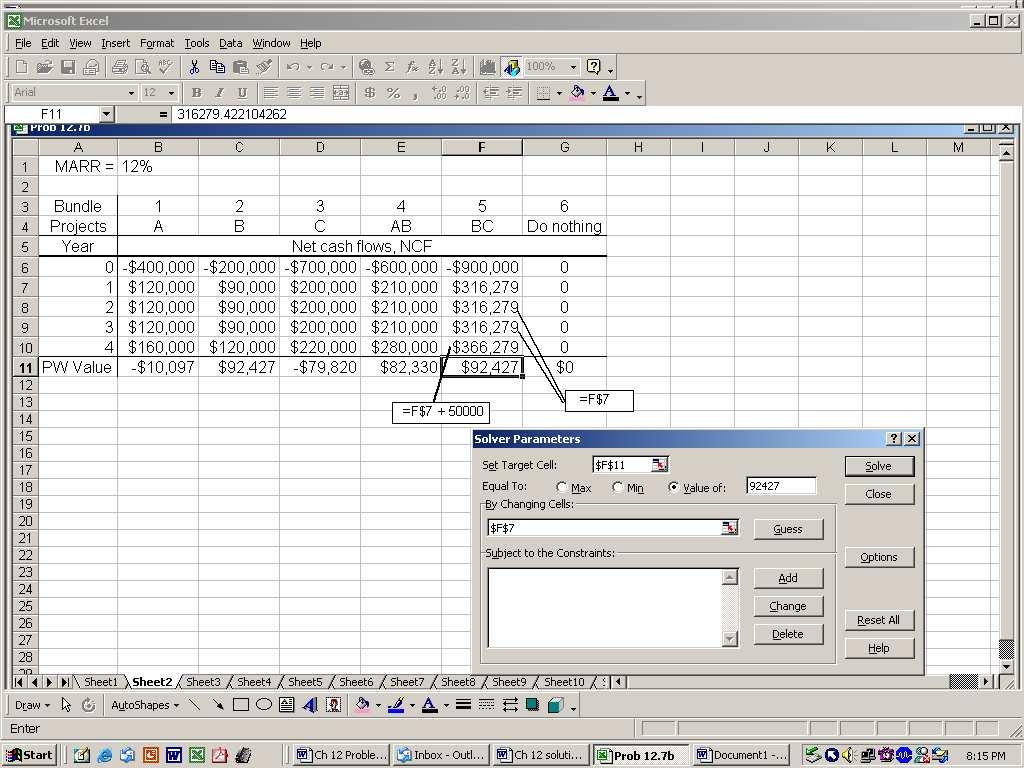
51

52 12.10 (a) Set up spreadsheet and determine that the Do Nothing bundle is the only acceptable one, and that PW C = $ Since the initial investment occurs at time t = 0, maximum initial investment for C at which PW = 0 is -550,000 + (-6219) = $-543,781 (b) Use SOLVER with the target cell as PW = 0 for project C. Result is MARR = 9.518%.

53 12.13 (a) PW values are determined at MARR = 15% per year. Initial NCF, Life, Bundle Projects investment, $ $ per year years PW at 15% mil 360,000 8 $115, , , , , , , , , , , , ,180, , , , ,340, , ,000 5 Select projects 1 and 4 with $3.5 million invested Budget limit, b = $16,000 MARR = 12% per year NCF for Bundle Projects Investment years 1 through 5 PW at 12% 1 1 $-5,000 $1000,1700,2400, $ , , ,500,500, , , ,5000, ,000 0,0,0, ,2-13, ,2200,2900, , ,3-14, ,6700,4400, , ,4-15, ,1700,2400, ,3800

54 12.19 (a) Select projects C and E. (b) Change MARR to 12% and the budget constraint to $500,000. Select projects A, C and E.

55 12.22 Select projects 1 and 4 with $3.5 million invested.

56 12.25 Use SOLVER repeatedly to find the best projects and corresponding value of Z. Develop an Excel chart for the two series.

57 SOLUTIONS TO SELECTED PROBLEMS Student: You should work the problem completely before referring to the solution. CHAPTER 13 Solutions included for problems: 1, 5, 8, 11, 14, 17, 21, 23b, (a) Q BE = 1,000,000/( ) = 235,294 units (b) Profit = 8.50Q 1,000, Q at 200,000 units: Profit = $-150,000 (loss) at 350,000 units: Profit = $487, From Equation [13.4], plot C u = 160,000/Q + 4. (a) If C u = $5, from the graph, Q is approximately 160,000. If Q is determined by Equation [13.4], it is 5 = 160,000/Q + 4 Q = 160,000/1 = 160,000 units (b) From the plot, or by equation, Q = 100,000 units. C u = 6 = 200,000/Q + 4 Q = 200,000/2 = 100,000 units 13.8 On spreadsheet for 13.7, include an IF statement for the computation of Q BE for the reduced FC of $750,000. The breakeven point reduces to 521,739.

58 13.11 FC = $305,000 v = $5500/unit (a) Profit = (r v)q FC 0 = (r 5500) ,000 (r 5500) = 305,000 / 5000 r = $5561 per unit (b) Profit = (r v)q FC 500,000 = (r 5500) ,000 (r 5500) = (500, ,000) / 8000 r = $5601 per unit Let x = hours per year -800(A/P,10%,3) - (300/2000)x -1.0x = -1,900(A/P,10%,5) - (700/8000)x - 1.0x -800( ) x - 1.0x = -1,900(0.2638) x - 1.0x x = 2873 hours per year (a) Let x = breakeven days per year. Use annual worth analysis. -125,000(A/P,12%,8) + 5,000(A/F,12%,8) - 2,000-40x = -45( x) -125,000(0.2013) + 5,000(0.0813) - 2,000-40x = x x = 24.6 days per year

59 (b) Since 75 > 24.6 days, buy. Annual cost is $-29, Let x = yards per year to breakeven (a) Solution by hand -40,000(A/P,8%,10) - 2,000 -(30/2500)x = - [6(14)/2500]x -40,000( ) - 2, x = x x = 368,574 yards per year (b) Solution by computer: There are many Excel set-ups to work the problem. One is: Enter the parameters for each alternative, including some number of yards per year as a guess. Use SOLVER to force the breakeven equation to equal 0, with a constraint that total yardage be the same for both alternatives (b) Enter the cash flows and develop the PW relations for each column. Breakeven is between 15 and 16 years. Selling price is estimated to be between $206,250 and $210,000.

60 13.26 (a) By hand: Let P = first cost of sandblasting. Equate the PW of painting each 4 years to PW of sandblasting each 10 years, up to 38 years. PW of painting PW p = -2,800-3,360(P/F,10%,4) - 4,032(P/F,10%,8) - 4,838(P/F,10%12) 5,806(P/F,10%,16) - 6,967(P/F,10%,20) -8,361(P/F,10%,24) 10,033(P/F,10%,28) - 12,039(P/F,10%,32) -14,447(P/F,10%,36) = $-13, (cont) PW of sandblasting PW s = -P - 1.4P(P/F,10%,10) P(P/F,10%,20) P(P/F,10%,30) -P[ (0.3855) (0.1486) (0.0573)] = P

61 Equate PW relations to obtain P = $6,739 (b) By computer: Enter the periodic costs. Use SOLVER to find breakeven at P = $6739. (c) Change MARR to 30% and 20%, respectively, and re-solver to get: 30%: P = -$ %: P = -$7546

62 SOLUTIONS TO SELECTED PROBLEMS Student: You should work the problem completely before referring to the solution. CHAPTER 14 Solutions included for problems 1, 4, 7, 10, 13, 16, 19, 22, 25, 28, 31, 34, 37, 40, 43, 46, and Inflated dollars are converted into constant value dollars by dividing by one plus the inflation rate per period for however many periods are involved Then-current dollars = 10,000( ) 10 = $19, CV 0 for amt in yr 1 = 13,000/( ) 1 = $12,264 CV 0 for amt in yr 2 = 13,000/( ) 2 = $11,570 CV 0 for amt in yr 3 = 13,000/( ) 3 = $10, (a) At a 56% increase, $1 would increase to $1.56. Let x = annual increase = (1 + x) = 1 + x = 1 + x x = 9.3% per year (b) Amount greater than inflation rate: = 6.8% per year i f = (0.04)(0.27) = 32.08% per year For this problem, i f = 4% per month and i = 0.5% per month 0.04 = f + (0.005)(f) 1.005f = f = 3.48% per month Buying power = 1,000,000/( ) 27 = $450,189

63 14.22 (a) PW A = -31,000 28,000(P/A,10%,5) (P/F,10%,5) = -31,000 28,000(3.7908) (0.6209) = $-134,038 PW B = -48,000 19,000(P/A,10%,5) (P/F,10%,5) = -48,000 19,000(3.7908) (0.6209) = $-115,679 Select Machine B (b) i f = (0.10)(0.03) = 13.3% PW A = -31,000 28,000(P/A,13.3%,5) (P/F,13.3%,5) = -31,000 28,000(3.4916) (0.5356) = $-126,087 PW B = -48,000 19,000(P/A,13.3%,5) (P/F,13.3%,5) = -48,000 19,000(3.4916) (0.5356) = $-110,591 Select machine B (a) New yield = = 5.18% per year (b) Interest received = 25,000(0.0518/12) = $ ,000 = 625,000(F/P,f,7) (F/P,f,7) = (1 + f) 7 = f = 2.44% per year In constant-value dollars, cost will be $40, Future amount is equal to a return of i f on its investment i f = ( ) ( )(0.03) = 17.42% Required future amt = 1,000,000(F/P,17.42%,4) = 1,000,000(1.9009) = $1,900,900 Company will get more; make the investment i f = (0.15)(0.06) = 21.9% AW = 183,000(A/P,21.9%,5) = 183,000( ) = $63,768

64 14.40 Find amount needed at 2% inflation rate and then find A using market rate. F = 15,000( ) 3 = 15,000( ) = $15,918 A = 15,918(A/F,8%,3) = 15,918( ) = $ (a) For CV dollars, use i = 12% per year AW A = -150,000(A/P,12%,5) 70, ,000(A/F,12%,5) = -150,000( ) 70, ,000( ) = $-105,315 AW B = -1,025,000(0.12) 5,000 = $-128,000 Select Machine A (b) For then-current dollars, use i f i f = (0.12)(0.07) = 19.84% AW A = -150,000(A/P,19.84%,5) 70, ,000(A/F,19.84%,5) = -150,000(0.3332) 70, ,000(0.1348) = $-114,588 AW B = -1,025,000(0.1984) 5,000 = $-208,360 Select Machine A Answer is (d) Answer is (a)

65 SOLUTIONS TO SELECTED PROBLEMS Student: You should work the problem completely before referring to the solution. CHAPTER 15 Solutions included for problems: 2, 4, 6, 10, 13, 16, 19, 22, 25, 28, 31, 34, 37, 40, 43, 46, 49, and The bottom-up approach uses price as output and cost estimates as inputs. The design-to-cost approach is just the opposite Property cost: (100 X 150)(2.50) = $37,500 House cost: (50 X 46)(.75)(125) = $215,625 Furnishings: (6)(3,000) = $18,000 Total cost: $271, Cost = 1200_ (78,000) = $91, (a) First find the percentage increase (p%) between 1990 and = 4732 (F/P,p,10) = (1+p) 10 p% increase = %/year Predicted index value in 2002 = 6221(F/P,2.773%,2) = 6571 (b) Difference = = Find the percentage increase between 1994 and = 368.1(F/P,p,8) = (1+p) 1/8 (1+p) = p % increase = % per year Index in 2005 = (F/P,2%,6) = C 2 = 13,000(450/250) 0.32 = $15, (a) 450,000 = 200,000(60,000/35,000) x 2.25 = x x = (b) Since x > 1.0, there is diseconomy of scale and the larger CFM capacity is more expensive than a linear relation would be.

66 15.25 (a) C 2 = (1 million)(3) 0.2 (1.1) = (1 million)(1.246)(1.1) = $1.37 million Estimate was $630,000 low (b) 2 million = (1 million)(3) x (1.25) 1.6 = (3) x x = ENR construction cost index ratio is (6538/4732). Cost -capacity exponent is Let C 1 = cost of 5,000 sq. m. structure in 1990 C 2 in 1990 = $220,000 = C 1 (10,000/5,000) 0.60 C 1 = $145,145 Update C 1 with cost index. C 2002 = C 1 (6538/4732) = $200, h = = 1.95 C T in 1994: 1.75 (1.95) = $3.41 million Update with the cost index to now. C T now: 3.41 (3713/2509) = 3.41(1.48) = $5.05 million Indirect cost rate for 1 = 50,000 = $ per hour 600 Indirect cost rate for 2 = 100,000 = $ per hour 200 Indirect cost rate for 3 = 150,000 = $ per hour 800 Indirect cost rate for 4 = 200,000 = $ per hour 1, Housing: DLH is basis; rate is $16.35 Actual charge = 16.35(480) = $7,848 Subassemblies: DLH is basis; rate is $16.35 Actual charge = 16.35(1,000) = $16,350 Final assembly: DLC is basis; rate is $0.23 Actual charge = 0.23 (12,460) = $2, DLC average rate = ( ) /3 = $3.483 per DLC $

67 Department 1: 3.483(20,000) = $ 69,660 Department 2: 3.483(35,000) = 121,905 Total actual charges: $1,068,584 Allocation variance = 800,000 1,068,584 = $-268, As the DL hours component decreases, the denominator in Eq. [15.7], basis level, will decrease. Thus, the rate for a department using automation to replace direct labor hours will increase in the computation DLH rate = $400,00/51,300 = $7.80 per hour Old cycle time rate = $400,000/97.3 = $4,111 per second New cycle time rate = $400,000/45.7 = $8, per second Actual charges = (rate)(basis level) Line DLH basis $156,000 99, ,080 Old cycle time 53, , ,164 New cycle time 34, , ,068 The actual charge patterns are significantly different for all 3 bases ,750 = 75,000(I 2 /1027) I 2 = 1229 Answer is (a) Cost now = 15,000(1164/1092) (2) 0.65 = $25,089 Answer is (b)

68 SOLUTIONS TO SELECTED PROBLEMS Student: You should work the problem completely before referring to the solution. CHAPTER 16 Solutions included for problems: 2, 4, 8, 11, 14, 17, 20, 23, 26, 29, 32, 35, 38, 41, and Book depreciation is used on internal financial records to reflect current capital investment in the asset. Tax depreciation is used to determine the annual taxdeductible amount. They are not necessarily the same amount Asset depreciation is a deductible amount in computing income taxes for a corporation, so the taxes will be reduced. Thus PW or AW may become positive when the taxes due are lower Part (a) Part (b) Book Annual Depreciation Year value depreciation rate 0 $100, ,000 $10, % 2 81, , , , (c) Book value = $59,049 and market value = $24,000. (d) Plot year versus book value in dollars for the table above

69 16.11 (a) D t = (12, )/8 = $1250 (b) BV 3 = 12,000 3(1250) = $8250 (c) d =1/n = 1/8 = (a) B = $50,000, n = 4, S = 0, d = 0.25 Accumulated Book Year Depreciation depreciation value $50,000 1 $12,500 $12,500 37, ,500 25,000 5, ,500 37,500 12, ,500 50,000 0 (b) S = $16,000; d = 0.25; (B - S) = $34,000 Accumulated Book Year Depreciation depreciation value $50,000 1 $8,500 $ 8,500 41, ,500 17,000 33, ,500 25,500 24, ,500 34,000 16,000

70 16.17 (a) B = $50,000, n = 3, d = for DDB Annual depreciation = X(BV of previous year) Accumulated Book Year Depreciation depreciation value $50,000 1 $33,335 $33,335 16, ,112 44,447 5, ,704 48,151 1,851 (b) Use the function =DDB(50000,0,3,t,2) for annual DDB depreciation.

71 16.20 SL: d t = 0.20 of B = $25,000 BV t = 25,000 - t(5,000) Fixed rate: DB with d = 0.25 DDB: d = 2/5 = 0.40 BV t = 25,000(0.75) t BV t = 25,000(0.60) t Declining balance methods Year SL 125% SL 200% SL d $25,000 $25,000 $25, ,000 18,750 15, ,000 14,062 9, ,000 10,547 5, ,000 7,910 3, ,933 1, (a) d = 1.5/12 = D 1 = 0.125(175,000)(0.875) 1 1 = $21,875 BV 1 = 175,000(0.875) 1 = $153,125 D 12 = $5,035 BV 12 = $35,248 (b) The 150% DB salvage value of $35,248 is larger than S = $32,000. (c) =DDB(175000,32000,12,t,1.5) for t = 1, 2,, B = $500,000; S = $100,000; n = 10 years SL: d = 1/n = 1/10 D 1 = (B-S)/n = (500, ,000)/10 = $40,000 DDB: d = 2/10 = 0.20 D 1 = db = 0.20(500,000) = $100, % DB: d = 1.5/10 = 0.15 D 1 = db = 0.15(500,000) = $75,000 MACRS: d = 0.10 D 1 = 0.10(500,000) = $50,000 First-year tax depreciation amounts vary considerably from $40,000 to $100, Classical SL, n = 5 D t = 450,000/5 = $90,000 BV 3 = 450,000 3(90,000) = $180, (cont) MACRS, after 3 years for n = 5 sum the rates in Table ΣD t = 450,000(0.712) = $320,400 BV 3 = $450, ,400 = $129,600

72 The difference is $50,400 that is not removed by classical SL Percentage depletion for copper is 15% of gross income, not to exceed 50% of taxable income. Use GI = (tons)($/pound)(2000 pounds/ton). Gross % Depl 50% Allowed Year 15% of TI depletion 1 $3,200,000 $480,000 $750,000 $480, ,020,000 1,053,000 1,000,000 1,000, ,990, , , , Depreciation factor is 17.49%. D = 35,000(0.1749) = $6122. Answer is (d) For SL method, BV at end of asset s life MUST equal salvage value of $10,000. Answer is (c) Straight line rate is always used as the reference. So, answer is (a)

73 SOLUTIONS TO SELECTED PROBLEMS Student: You should work the problem completely before referring to the solution. CHAPTER 17 Solutions included for all or part of problems: 4, 6, 9, 12, 15, 18, 21, 24, 27, 29, 33, 36, 39, 42, 45, 48, 51, 54, 57, and (a) Company 1 TI = (1,500, ,000) 754, ,000 = $629,000 Taxes = 113, (629, ,000) = $213,860 Company 2 TI = $236,000 Taxes = $75,290 (b) Co. 1: 213,860/1.5 million = 14.26% Co. 2: 75,290/820,000 = 9.2% (c) Company 1 Taxes = (TI)(T e ) = 629,000(0.34) = $213,860 % error with graduated tax = 0% Company 2 Taxes = 236,000(0.34) = $80,240 % error = + 6.6% 17.6 T e = ( )(0.34) = TI = $2.4 million Taxes = 2,400,000(0.390) = $936, (a) GI = 98, = $105,500 TI = 105,500 10,500 = $95,000 Taxes = 0.10(7000) (21,400) (40,400) (26,200) = $21,346 (b) 21,346/98,000 = 21.8% (c) Reduced taxes = 0.9(21,346) = $19,211 $19,211 = 0.10(7000) (21,400) (40,400) (TI 26,200) = , (x 68,800) = 14, (x 68,800) 0.28x = 24,465 x = $87,375

74 Let y = new total of exemptions and deductions TI = 87,375 = 105,500 y y = $18,125 Total must increase from $10,500 to $18,125, which is a 73% increase Depreciation is used to find TI. Depreciation is not a true cash flow, and as such is not a direct reduction when determining either CFBT or CFAT CFBT = CFAT + taxes = [CFAT D(T e )]/(1 T e ) T e = (0.35) = CFBT = [2,000,000 (1,000,000)( )]/( ) = $2,610, (a) BV 2 = 80,000 16,000 25,600 = $38,400 (b) P or Year (GI E) S D TI Taxes CFAT 0-80, $80, ,000 16,000 34,000 12,920 37, ,000 38,400 25,600 24,400 9,272 79, Here Taxes = (CFBT depr)(tax rate). Select the SL method with n = 5 years.

75 17.24 (a) t=n PW TS = (tax savings in year t)(p/f,i,t) t=1 Select the method that maximizes PW TS. (b) TS t = D t (0.42). PW TS = $27,963 Year,t d Depr TS $26,664 $11, ,560 14, ,848 4, ,928 2, (a) CL = = $4500 TI = $ 4500 Tax savings = 0.40( 4500) = $ 1800 (b) CG = $10,000 DR = 0.2(100,000) = $20,000 TI = CG + DR = $30,000 Taxes = 30,000(0.4) = $12,000

76 17.29 (a) BV 2 = 40, (40,000) = $19,200 DR = 21,000 19,200 = $1800 TI = GI E D + DR = $6,000 Taxes = 6,000(0.35) = $2100 (b) CFAT = 20, , = $35, In brief, net all short term, then all long term gains and losses. Finally, net the gains and losses to determine what is reported on the return and how it is taxed = 0.12(1-tax rate) Tax rate = Since MARR = 25% exceeds the incremental i* of 17.26%, the incremental investment is not justified. Sell NE now, retain TSE for the 4 years and then dispose of it (a) PW A = -15, (P/A,14%,10) (P/F,14%,10) = $-29,839 PW B = -22, (P/A,14%,10) (P/F,14%,10) = $-28,476

77 Select B with a slightly smaller PW value. (b) Machine A Annual depreciation = (15,000 3,000)/10 = $1200 Tax savings = 4200(0.5) = $2100 CFAT = = $ 900 PW A = 15, (P/A,7%,10) (P/F,7%,10) = $ 19,796 Machine B Annual depreciation = $1700 Tax savings = $1600 CFAT = = $100 Select machine B PW B = 22, (P/A,7%,10) (P/F,7%,10) = $ 18,756 (c) Machine A Year P or S AOC Depr Tax savings CFAT 0 $ 15, $ 15,000 1 $3000 $3000 $ (cont) Machine B Year P or S AOC Depr Tax savings CFAT 0 $ 22, $ 22,000 1 $1500 $4400 $

78 PW A = $ 18,536. PW B = $ 16,850. Select machine B, as above (b 1 and 2) (a) From Problem 17.42(b) for years 1 through 10. CFAT A = $ 900 CFAT B = $+100 Use a spreadsheet to find the incremental ROR and to determine the PW of incremental CFAT versus incremental i values. If MARR < 9.75%, select B, otherwise select A.

79 (b) Use the PW vs. incremental i plot to select between A and B. MARR Select 5% B 9 B 10 A 12 A Defender Annual SL depreciation = 450,000 /12 = $37,500 Annual tax savings = (37, ,000)(0.32) = $63,200 AW D = -50,000(A/P,10%,5) 160, ,200 = $ 109,990 Challenger Book value of D = 450,000 7(37,500) = $187,500 CL from sale of D = BV 7 Market value = $137,500 Tax savings from CL, year 0 = 137,500(0.32) = $44,000 Challenger annual SL depreciation = $65,000 Annual tax saving = (65, ,000)(0.32) = $68,800 AW C = $-184,827 Select the defender. Decision was incorrect.

80 17.54 Succession options Option Defender Challenger 1 2 years 1 year Defender AW D1 = $300,000 AW D2 = $240,000 Challenger No tax effect if defender is cancelled. Calculate CFAT for 1, 2, and 3 years of ownership. Tax rate is 35%. Year 1: TI = 120, , ,640 = $ 320,000 Year 2: TI = 120, , ,240 = $ 253,360 Year 3: TI = 120, , ,720 = $ 97,760 Year 1: CFAT = 120, ,000 ( 112,000) = $592,000 Year 2: CFAT = -120, ,000 (-88,676) = $368,676 Year 3: CFAT = -120, ,000 (-34,216) = $114,216 AW C1 = $ 288,000 AW C2 = $+24,696 AW C3 = $+51,740 Selection of best option: Replace now with the challenger. Year Option AW 1 $ 240,000 $ 240,000 $ 288,000 $ 254, ,000 24,696 24,696 94, ,740 51,740 51, , (a) Before taxes: Let RV = 0 to start and establish CFAT column and AW of CFAT series. If tax rate is 0%, RV = $415,668.

81 17.60 (a) Take TI, taxes and D from Example Use i = 0.10 and T e = 0.35.

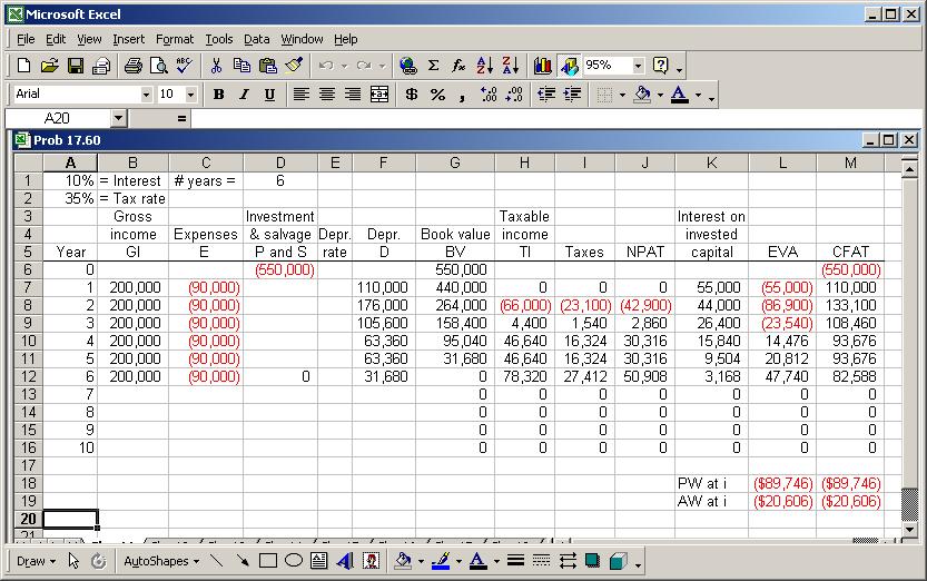
82

83 SOLUTIONS TO SELECTED PROBLEMS Student: You should work the problem completely before referring to the solution. CHAPTER 18 Solutions included for problems: 1, 4, 7, 10, 13, 16, 19, 22, 25, 29, 31, and tons/day: PW = 62, P/F,10%,8) 0.50(10)(200)(P/A,10%,8) 4(8)(200)(P/A,10%,8) = $ 100, tons/day: PW = $ 140, tons/day: PW = $ 213, PW Build = 80,000 70(1000) + 120,000(P/F,20%,3) = $-80,556 PW Lease = (2.5)(12)(1000) (2.50)(12)(1000)(P/A,20%,2) = $ 75,834 Lease the space. New construction cost = 70(0.90) = $63 and lease at $2.75 PW Build = $ 73,556 PW Lease = $ 83,417 Select build. The decision is sensitive (a) Breakeven number of vacation days per year is x. AW cabin = 130,000(A/P,10%,10) + 145,000(A/F,10%,10) x (50/30) (1.20)x AW trailer = 75,000(A/P,10%,10) + 20,000(A/F,10%,10) 1, x [300/30(0.6)](1.20)x AW cabin = AW trailer x = days (Use x = 20 days per year) (b) Determine AW for 12, 16, 20, 24, and 28 days. AW cabin = 13, x AW trailer = 12, x Days, x AW cabin AW trailer Selected 12 $-11,783 $-11,441 Trailer 16-11,191-11,021 Trailer

84 20-10,599-10,601 Cabin 24-10,007-10,181 Cabin Cabin Each pair of AW values are close to each other, especially for x = For spreadsheet analysis, use the PMT functions to obtain the AW for each n value for each G amount. The AW curves are quite flat; there are only a few dollars difference for the various n values around the n* value for each gradient value.

85 18.13 (a) First cost sensitivity: AW = P( ) + 24,425 (b) AOC sensitivity: AW = AOC + 21,624 (c) Revenue sensitivity: AW = 32,376 + Revenue Water/wastewater cost = ( ) per 1000 liters = 0.16 per 1000 liters Spray Method Pessimistic liters Water required = 10,000,000(100) = 1.0 billion AW = (0.16/1000)(1.00 X 10 9 ) = $ 160,000 Most Likely - 80 liters Water required = 10,000,000(80) = 800 million AW = (0.16/1000)(800,000,000) = $ 128,000 Optimistic - 40 liters Water required = 10,000,000(40) = 400 million AW = (0.16/1000)(400,000,000) = $ 64,000 Immersion Method AW = 10,000,000(40)(0.16/1000) 2000(A/P,15%,10) 100 = $ 64,499 Immersion method is cheaper, unless optimistic estimate of 40 L is the actual (a) E(time) = (1/4)( ) = 32.5 seconds

86 (b) E(time) = 20 seconds The 70 second estimate does increase the mean significantly E(i) = 103/20 = 5.15% E(revenue) = $222,000 E(AW) = 375,000(A/P,12%,10) 25,000[(P/F,12%,4) + (P/F,12%,8)] (A/P,12%,10) 56, ,000 = $95,034 Construct mock mountain AW = annual loan payment + (damage) x P(rainfall amount or greater) Subscript on AW indicates the rainfall amount. AW 2.00 = $ 42,174 AW 2.25 = $ 35,571 AW 2.50 = $ 43,261 AW 3.00 = $ 54,848 AW 3.25 = $ 61,392 Build a wall to protect against a rainfall of 2.25 inches with an expected AW of $ 35, D3: Top: E(value) = $30 Bottom: E(value) = $10 Select top at D3 for $30 D1: Top: Value at D1 = = $27 Bottom: = $10 Select top at D1 for $27 D2: Top: E(value) = $66 Middle: E(value) = 0.5( ) = $50 Bottom: E(value) = $ (cont) At D2, value = E(value) investment Top: = $41 Middle: = $20 Bottom: = $30 Select top at D2 for $41

87 Conclusion: Select D2 path and choose top branch ($25 investment) (a) Construct the decision tree. (b) Expansion option (PW for D2, $120,000) = $4352 (PW for D2, $140,000) = $21,744 (PW for D2, $175,000) = $52,180 E(PW) = $28, (cont) No expansion option (PW for D2, $100,000 = $86,960 E(PW) = $86,960 Conclusion at D2: Select no expansion option (c) Complete foldback to D1.

88 Produce option, D1 E(PW of cash flows) = $202,063 E(PW for produce) = $ 47,937 Buy option, D1 At D2, E(PW) = $86,960 E(PW for buy)= cost + E(PW of sales cash flows) = 450, (PW sales up) (PW sales down) = 450, (228,320) (195,660) = $ 236,377 Conclusion: Both returns are less than 15%, but the expected return is larger for produce option than buy. (d) The return would increase on the initial investment, but would increase faster for the produce option.

89 SOLUTIONS TO SELECTED PROBLEMS Student: You should work the problem completely before referring to the solution. CHAPTER 19 Solutions included for problems: 2, 5, 8, 11, 14, 17, and Needed or assumed information to be able to calculate an expected value: 1. Treat output as discrete or continuous variable. 2. If discrete, center points on cells, e.g., 800, 1500, and 2200 units per week. 3. Probability estimates for < 1000 and /or > 2000 units per week (a) P(N) = (0.5) N N = 1,2,3,... is discrete N etc. P(N) F(N) P(L) is a triangular distribution with the mode at 5. f(mode) = f(m) = 2 = F(mode) = F(M) = 5-2 = (b) P(N = 1, 2 or 3) = F(N 3) = (a) X i F(X i ) (b) P(6 X 10) = F(10) F(3) = = 0.4 P(X = 4, 5 or 6) = F(6) F(3) = = 0.1 (c) P(X = 7 or 8) = F(8) F(6) = = 0.0 No sample values in the 50 have X = 7 or 8. A larger sample is needed to observe all values of X.

90 19.11 Use the steps in Section As an illustration, assume the probabilities that are assigned by a student are: 0.30 G=A 0.40 G=B P(G = g) = 0.20 G=C 0.10 G=D 0.00 G=F 0.00 G=I Steps 1 and 2: The F(G) and RN assignment are: RNs 0.30 G=A G=B F(G = g) = 0.90 G=C G=D G=F G=I -- Steps 3 and 4: Develop a scheme for selecting the RNs from Table Assume you want 25 values. For example, if RN 1 = 39, the value of G is B. Repeat for sample of 25 grades. Step 5: Count the number of grades A through D, calculate the probability of each as count/25, and plot the probability distribution for grades A through I. Compare these probabilities with P(G = g) above (a) Convert P(X) data to frequency values to determine s. X P(X) XP(X) f X 2 fx Sample average: Xbar = 4.6 Sample variance: s 2 = (4.6) 2 = s = (cont) (b) Xbar ± 1s is 4.6 ± 3.42 = 1.18 and values, or 50%, are in this range.

91 19.17 P(N) = (0.5) N Xbar ± 2s is 4.6 ± 6.84 = 2.24 and All 50 values, or 100%, are in this range. E(N) = 1(.5) + 2(.25) + 3(.125) + 4(0.625) + 5(.03125) + 6( ) + 7( ) + 8( ) + 9( ) + 10( ) +.. = The limit to the series N(0.5) N is 2.0, the correct answer Use the spreadsheet Random Number Generator (RNG) on the tools toolbar to generate CFAT values in column D from a normal distribution with µ = $2040 and σ = $500. The RNG screen image is shown below. (This tool may not be available on all spreadsheets.) (cont)

92 The decision to accept the plan uses the logic: Conclusion: For certainty, accept the plan if PW > $0 at MARR of 7% per year. For risk, the result depends on the preponderance of positive PW values from the simulation, and the distribution of PW obtained.