36106 Managerial Decision Modeling Monte Carlo Simulation in Excel: Part II

Transcription

1 36106 Managerial Decision Modeling Monte Carlo Simulation in Excel: Part II Kipp Martin University of Chicago Booth School of Business November 8, 2017

2 Reading and Excel Files Reading: Powell and Baker: Chapter 14.4 See the handout for Week Eight: TIAA-CREF Simulation Model See the Documentation and Examples folders in the Palisade RISK7 directory that was installed with your software.

3 Learning Objectives 1. Learn to Analyze the Tail of a Distribution Use RiskTarget 2. Use Simulation to value an IPO (Netscape) 3. Learn to use compound statistical distributions 4. Learn to run multiple simulations to optimize.

4 Reading and Excel Files 4 Files used in this lecture: riskstatic.xlsx retirement TIAA.xlsx retirement TIAA key.xlsx Ch14-4CorporateValuationBaseModelEmpty.xlsx (Canvas) Ch14-4CorporateValuationBaseModel.xlsx (Canvas) Ch14-4CorporateValuationSensitivityModel.xlsx (Canvas) Ch14-4CorporateValuationRiskModel.xlsx (Canvas) compounddistributions.xlsx compounddistributions key.xlsx retirementrisktable.xlsx retirementrisktable key.xlsx airlineoverbooking.xlsx airlineoverbooking key.xlsx

5 Lecture Outline 5 Brief Review Analyze Distribution Tails TIAA/CREF Corporate Valuation (Netscape) Compound Distributions Multiple Simulations (RiskSimtable) Airline Overbooking

6 Review Key Concepts: Using an expected value E(X ), instead of a distribution X, is bad. Nonlinearity can make this even worse (Excel functions like IF, MAX, MIN, are serious offenders) Big standard deviations can make this even worse. we can insert an X into the spreadsheet instead of E(X ) and run trials for different values of gives us E(f (X )) instead of f (E(X )).

7 Review We are taking tools from earlier in the quarter and extending them to allow for stochastic parameters. Goal Goal Seek (Last Week) Data RiskSimtable (This Week) Optimizer (Week Ten)

8 Review We used Define Distributions to put in a distribution. Other options include: Use the Insert Function Just type it in (there is auto completion available) IMPORTANT: Please do not set RiskStatic(). Use default value which is: for a continuous distribution (e.g. RiskNormal or RiskUniform) the mean of the distribution for a discrete distribution (RiskDiscrete) the distribution value closest to the mean Note: the number you see in a simulation cell is the result of the last trial.

9 Review See the spreadsheet riskstatic.xlsx which illustrates the RiskStatic function for the RiskDiscrete() and RiskUniform() distributions. Here is how to force a value for RiskStatic(). Setting RiskStatic() for the RiskDiscrete distribution =RiskDiscrete(C4:C8,D4:D8, RiskStatic(50)) Setting RiskStatic() for the RiskUniform distribution =RiskUniform(C19,D19, RiskStatic(107.36))

10 Review 10 Skills: 1. Be able to insert a distribution 2. Run (and stop) and set simulation parameters 3. Be able to generate a histogram of results (use Add Output) 4. Be able to analyze results 5. simulation functions in your workbook, e.g. RiskMean 6. Goal Seek

11 Analyze Distribution Tails TIAA/CREF Key Idea: we are often interested in the tail of a simulation distribution. We illustrate with an example from TIAA/CREF Financial Services. A large provider for people working in education, research, and medicine. In this exercise we show how TIAA/CREF provides analysis of the tail of a simulation distribution for clients. See also the handout under Week 7. coursework/36106/handouts/retirement-portfolio.pdf

12 12 Analyze Distribution Tails Here is part of an actual report from TIAA-CREF.

13 Analyze Distribution Tails TIAA/CREF Three Key Points: 1. We evaluated the results of 500 hypothetical simulations reflecting various possible market conditions. 2. The analysis is performed to simulate a number of possible financial outcomes, rather than assuming an average return year after year. 3. For this analysis, we define success as being able to cover 90% or more of your goal in at least 450 trials. Note: results based on life expectancy and how aggressive the portfolio is.

14 Analyze Distribution Tails TIAA/CREF Goal: withdraw X dollars every year for N years and be left with Y dollars X a number selected by the user, for example $25,000 per year. Y a number selected by the user, for example $50,000 N life expectancy minus age at retirement Objective: Build model to find out often we meet 90% or more of our goal.

15 Analyze Distribution Tails TIAA/CREF 15 Open retirement TIAA. Use the data: 401 K Savings $200,000 Years 20 µ 11.55% σ % Payment Goal $25,000 per year Horizon End Goal $50,000 Goal Percentage 90% Key Question: what do we mean by meeting 90% or more of the goal?

16 Analyze Distribution Tails TIAA/CREF Key Question: what do we mean by meeting 90% or more of the goal? I assume we mean that: 1. For each of the 20 years there are sufficient funds to withdraw $25, After 20 years I have at least , 000 = 45, 000 dollars in my account. Now implement

17 Analyze Distribution Tails TIAA/CREF 17 We do the following: 1. Run a simulation that records how much money we have after 20 years. The simulation gives a distribution of returns. 2. Find the probability associated with a tail value of $45, Multiply the probability associated with the tail by the number of trials. We to calculate the tail probability we want. The use is illustrated spreadsheet RiskTarget in the retirement TIAA workbook

18 Analyze Distribution Tails TIAA/CREF 18

19 Analyze Distribution Tails TIAA/CREF 19

20 Analyze Distribution Tails TIAA/CREF 20 We implement two ways. Method 1: Use the RiskTargetD (descending CDF) function.

21 Analyze Distribution Tails TIAA/CREF In cell E38 we put =RiskTargetD(E35,risk_target,1)*num_iterations This is what the TIAA CREF report is doing when they say: In 494 trials, 90% or more of your goal was covered. What is our number?

22 Analyze Distribution Tails TIAA/CREF We implement two ways. Method 2: Requires three steps. Step 1: First, count whether or not we meet our goal using an IF statement. =IF(E35 >= risk_target,1,0) Step 2: Build a distribution of the simulation results on the IF statement. We get a bimodal distribution. Either a 0 or 1. What does the resulting histogram tell you? (See Figure next page) What does the mean tell you?

23 Analyze Distribution Tails TIAA/CREF 23

24 Analyze Distribution Tails TIAA/CREF Step 2 (Continued): Build a distribution for the IF. =RiskOutput()+IF(E35 >= risk_target,1,0) Step 3: Get the mean of this distribution using RiskMean. =RiskMean(E39,1)*num_iteration

25 Analyze Distribution Tails TIAA/CREF 25

26 Corporate Valuation This comes from Powell and Baker, Section The initial IPO for Netscape was August 9, The underwriters, led by Morgan Stanley & Company, offered five million shares at $28 per share. This was the beginning of the Internet boom. At $28 per share, Netscape s market value would be more than $1 billion dollars despite a book value of $16 million Microsoft copied the Netscape technology and developed Internet Explorer. They gave Internet Explorer away for free leading to a major legal battle. Our Objective: Place a value on Netscape given August, 1995 data.

27 Corporate Valuation The Plan: 1. Define the problem put a valuation on the firm (Netscape) 2. Assume all parameters (e.g. revenue growth rate) are deterministic 3. Calculate the NPV of the firm based on free cash flow 4. Determine the sensitivity of the NPV calculation to the inputs 5. Treat the most sensitive inputs as stochastic parameters (i.e. distributions) 6. Run a simulation

28 Corporate Valuation Spreadsheet Walk Through: 1. Ch14-4CorporateValuationBaseModelEmpty.xlsx (contains parameter assumptions) 2. Ch14-4CorporateValuationBaseModel.xlsx (the deterministic valuation model) 3. Ch14-4CorporateValuationSensitivityModel.xlsx (used for Step 5 in the previous slide) 4. Ch14-4CorporateValuationRiskModel.xlsx (used for Step 6 in the previous slide)

29 29 Corporate Valuation The basic assumptions for the deterministic model are given below. See Workbook Ch14-4CorporateValuationBaseModelEmpty.xlsx.

30 30 Corporate Valuation First, create the deterministic model. You will start with something like the following for homework.

31 31 Then fill in the numbers. Corporate Valuation

32 Corporate Valuation Full disclosure: I was a math major. Please do not ask me to justify accounting measures. We need to calculate the free cash flow in an income statement. The free cash flow is the amount of cash a company can generate after paying out the capital expenditures. See: Free cash flow is net income plus depreciation minus capital expenditure and changes in net working capital.

33 Corporate Valuation Objective: Calculate the present value of free cash flow. This requires the following key steps. 1. Calculate the present value of the free cash flow for the current year 1995 and the forecasted years Calculate the terminal value for the firm at the end of year Calculate the present value of the terminal value. 4. Add Steps 1 and 3 for the net present value. This number goes in cell B37 and the value is $1,203,357 (In the book you will see a value of present value calculation of $1,057,167. This is an error and was caught by Professor Che-Lin Su.)

34 Corporate Valuation Step 1: Calculate the present value of the free cash flow for the forecasted years (i.e. through the end of 2005.) Let C t denote the free cash flow at the end of period t. We know C 1995, this value is in cell B33 and is equal to (20,738). We have projected values for the 10-year period 1996 through These numbers are in the range C33:L33.

35 Corporate Valuation Step 1 (Continued): Calculate the present value of the free cash flow for the forecasted years (i.e. through the end of 2005.) Hence the present value of these cash flows is C t=1996 C t /(1 + i) This number is $243,196 and appears in cell B35. The formula in B35 is =B33+NPV(B16,C33:L33) The number i is cost of equity. In our spreadsheet this number is equal to 17.96% and is in cell B16.

36 Corporate Valuation Step 2: Calculate the terminal value. Use the Gordon terminal value. See axzz2ms2bjicl. The forecasts are through the end of However, we assume the firm has an infinite life. Let α be the terminal growth rate of free cash flow through infinity. In our case α = 0.04 and is given in cell B5. This implies the following values for fresh cash flow starting at the end of (1 + α)c 2005 (1 + α) 2 C 2005 (1 + α) 3 C 2005 (1 + α) 4 C 2005

37 Corporate Valuation Step 2 (Continued): Calculate the terminal value. Now discount these free cash flows back to the end of 2005 using the cost of equity (denoted by i) (1+α) (1+i) C 2005 (1+α) 2 (1+α) (1+i) C 3 (1+α) (1+i) C (1+i) C So we need to find C 2005 t=1 (1 + α) t (1 + i) t which is all future free cash flow discounted back to the end of 2005.

38 Corporate Valuation Step 2 (Continued): Calculate the terminal value. When 0 < r < 1, r t = r 1 r t=1 As long as α < i, 0 < (1 + α)/(1 + i) < 1. Doing a little algebra gives C 2005 t=1 (1 + α) t 1 + α (1 + i) t = C 2005 i α This is the number calculated in cell B34 with the formula =(L33*(1+B5))/(B16-B5) using range names gives =(c_2005*(1+alpha))/(i-alpha)

39 Corporate Valuation Step 2 (Continued): Calculate the terminal value. We have now discounted all future cash flows back to the end of Discount back to the end of This is ( ) 1 + α C 2005 /(1 + i) 10 i α This calculation is in cell B36 and gives $960,160. This differs from the value in the text, where the authors use a discount factor of (1 + i) 11. Professor Che-Lin the author of the above derivation found this error.

40 Corporate Valuation Excellent reference: Financial Modeling by Simon Benninga, MIT Press, ISBN (Third Edition). See Chapter 3, Financial Statement Modeling.

41 Corporate Valuation 41 You should understand the key part of the spreadsheet highlighted in gray below.

42 Corporate Valuation Deterministic Result: With the deterministic assumptions in the model, the NPV of Netscape is $1,203,357. See cell B37. This results in a price per share of $ See cell B44. Let s do a simulation on the NPV.

43 Corporate Valuation The first step is to determine which parameters have the greatest effect on the NPV outcome. We will create a tornado chart.

44 Corporate Valuation I did a sensitivity analysis on the following: Revenue growth rate alpha terminal value growth rate Cost of sales R&D (% of revenue) Tax Rate Depreciation Beta Riskless rate Market Risk Premium

45 Corporate Valuation 45 The settings for cell B6, Cost of sales (% revenues)

46 Corporate Valuation Disclaimer: This sensitivity analysis looks at changing only one parameter at a time. We do not change two or more parameters simultaneously.

47 47 The tornado chart. Corporate Valuation

48 Corporate Valuation Now identify key uncertainties. Based on the tornado chart we examine: Revenue Growth Rate assume normal with mean of 65 percent and standard deviation of 5 percent R&D (% of Revenue) assume triangular, with a minimum of 32 percent, most likely value of 37 percent, and a maximum of 42 percent Market Risk Premium assume uniform with a minimum of 5 percent and maximum of 10 percent

49 Corporate Valuation 49 Next identify model outputs. These are in the range B40:B44. See below.

50 Corporate Valuation 50 Run the simulation for 1000 trials. I get the following results: Output Mean Min Max Std. Dev. Total NPV 1,314, ,728 4,398, ,383 Ratio TV/Total NPV Year FCF > Max Loss -173, , ,408 13,723 Price/Share

51 Corporate Valuation At Canvas please go to Homework 7. Get the file FigureOddsInAcquisitionResults.pdf You will use this file and a corresponding Excel data file MergersandAcquisitionsData.xlsx to build a corporate valuation model. You will use FigureOddsInAcquisitionResults.pdf and the Excel file to get the time 0 data and assumptions about growth rates. You will then run a simulation based on stochastic parameter assumptions.

52 Corporate Valuation Important: Please note the following for your homework on M&A. See Point 6 in the M&A clarifications homework. The Capital Expenditures in the Ch14-4CorprateValuationBaseModel.xlsx example are calculated differently than in the M&A homework case. See Point 7 in the M&A clarifications homework. Calculate taxes and net income as in the Ch14-4CorprateValuationBaseModel.xlsx workbook.

53 Compound Distributions 53 Consider the following scenario: (sales, general, and administrative expenses (SG&A) from your next homework) 1. nature determines an outcome 2. for each possible outcome there is a (potentially different) probability distribution Example Data: Uniform Distribution Scenario Parameters Index Probability Min Max % 1% % 4% % 7%

54 Compound Distributions Example 1: Nature determines outcome state 1. In this case the relevant distribution is a uniform distribution with a min of -2% and a max of 1%. Example 2: Nature determines outcome state 3. In this case the relevant distribution is a uniform distribution with a min of 4% and a max of 7%. The probability of outcome (scenario) 1 is 0.3, the probability of outcome 2 is 0.5, and the probability of outcome 3 is 0.2. We want to model this process for seven years. You have to do this is in Homework 7, involving Mergers and Acquisitions. It is based on a document about probability-based scenario planning prepared by Crédit Lyonnais (now Crédit Agricole) of America.

55 Compound Distributions There are two methods in compounddistributions.xlsx to do this. Method 1: Step 1: For each year, generate a realization of each of the three random variables. For example, For example, the second number generated in Year Three, , is a realization from the uniform distribution with minimum 1% and maximum 4%.

56 Compound Distributions Important: 1. In the first part of this example, I am generating a different uniform distribution for each of the seven years, but we do not do that in the M&A case. In the M&A it is stipulated which years use the same draw from the uniform distribution. 2. In the M&A case we are using different draws from the RiskDiscrete for each of the different accounting measures, e.g. revenue growth, we may wish to use the SAME scenario probabilities for each accounting measure.

57 Compound Distributions Method 1 (continued): The first number generated in Year Five, , is a realization from the uniform distribution with minimum -2% and maximum 1%. Step 2: For each year, generate a realization from the RiskDiscrete random variable. For example, in the fourth row for Year One we have: =RiskDiscrete(C20:C22,probRange) The range probrange contains the probabilities.3,.5, and.2. Note that C20:C22 is the range with the realizations from the uniform distributions for year one.

58 Compound Distributions 58 Now do the experiment where we fix in F12:F14 the same uniform distribution to be used in each year. Then generate the output for years 1-7 in row 27. This is the way to do it for the M&A case.

59 59 Compound Distributions The histogram below illustrates that 30% of returns are between -2% and 1%. Note: we put an RiskOutput in for the RiskDiscrete in Period 1

60 Compound Distributions 60 The histogram below illustrates that 50% of returns are between 1% and 4%.

61 Compound Distributions 61 The cumulative distribution motivates the second approach.

62 Compound Distributions Method 2: Use function Riskcumul. For this function to be valid: 1. the probability distributions for each possible outcome must be uniform 2. the intervals defining the uniform distributions cannot overlap See the explanation and definition in the section Distribution Functions of the User s Manual.

63 Compound Distributions Method 2: (Continued) Riskcumul requires the following arguments: 1. a minimum value in our case (this is the minimum value of any realization over the set of uniform distributions) 2. a maximum value in our case 0.07 (this is the maximum value of any realization over the set of uniform distributions) 3. a range of X values in our case 0.01 and 0.04 (the upper limits of the uniform distributions, not including the uniform distribution that gave the maximum value) 4. a range of p values in our case 0.3 and 0.8 (the cumulative probabilities associated with the X values)

64 Compound Distributions 64 Method 2: (Continued) Defining Riskcumul

65 Compound Distributions 65 Method 2: (Continued) Riskcumul simulation results.

66 Compound Distributions Practice Problem: Assume there are two outcome distributions. Outcome 1: 25 percent probability that this outcome occurs this outcome results in a uniform distribution between -12 and -7 Outcome 2: 75 percent probability that this outcome occurs this outcome results in a uniform distribution between 0 and 8 Implement in Riskcumul. See

67 Compound Distributions Summary: Method 1: The Good: this is the most general method. No assumptions are made about the distributions associated with each outcome. They do not even need to be uniform. The Bad: The most cumbersome of the three methods to implement. Method 2: The Good: You can use a function, Riskcumul, nothing else needed. The Bad: The most restrictive of the three methods. The outcome distributions must be non-overlapping uniform distributions.

68 Multiple Simulations (RiskSimtable) New Idea: Return to the retirement example and treat the payment value as a variable. Run a simulation for different values of this variable. The current annual payment is $23, We currently take this as a given. Let s examine what happens as we vary this from $10,000 to $28,000. We are now treating the payment as adjustable or a variable. Remember the Data Table in the What If Analysis? We do a similar thing for simulation using RiskSimtable().

69 Multiple Simulations (RiskSimtable) The end result of this will be retirementrisktable key.xlsx. For now, modify retirementrisktable.xlsx. We had in B6 (the range payment) the value that results from evaluating the Excel PMT function. Treat this as a variable. Insert the RiskSimtable() function here. Under Insert Function select Special and then RiskSimtable(). See next slide for picture.

70 70 Multiple Simulations (RiskSimtable) Here is the location of RiskSimTable.

71 Multiple Simulations (RiskSimtable) 71 Now select the range where the test values are. In our case this is J8:J17.

72 72 Multiple Simulations (RiskSimtable) In columns J8:J17 we put the numbers 10,000 to 28,000 in increments of 2,000.

73 Multiple Simulations (RiskSimtable) Next in columns K, L, M, N and Row 8 we insert the four functions: =RiskMean(objectiveCell,I8) =RiskStdDev(objectiveCell,I8) =RiskMin(objectiveCell,I8) =RiskMax(objectiveCell,I8) Recall that objectivecell is the green cell E32, it is the Risk Output cell =RiskOutput()+COUNTIF(E12:E31,">0") Copy and paste the four functions through row 17.

74 Multiple Simulations (RiskSimtable) 74 The functions that we inserted came from Insert Function, Statistic Functions, then Simulation Result.

75 Multiple Simulations (RiskSimtable) 75 Now run 10 simulations since there are 10 possible values for our decision variables.

76 Multiple Simulations (RiskSimtable) 76 The simulation result is: Are the results logical?

77 Multiple Simulations (RiskSimtable) 77 You get a histogram for each simulation run. See the cute little icon.

78 Multiple Simulations (RiskSimtable) 78 A useful trick for getting rid of your simulation results. Under Utilities select Data...

79 Airline Overbooking See Excel files airlineoverbooking.xlsx and airlineoverbooking key.xlsx. This example is due to Sudhakar D. Deshmukh at Kellogg School of Management, Northwestern University. Consider the Chicago to Tokyo leg for North East Airlines (NEA). Chicago to Tokyo leg serviced by an NEA Boeing 007 jumbo jet with 300 passenger capacity. Each one-way ticket generates $500. The flight fixed cost is $80,000. Based on past data, there is a 10% chance a ticket holder does show. NEA is allowed to overbook, but must give $250 in compensation, plus provide alternative transportation which also costs $500. NEA wants to determine how many tickets to sell.

80 Airline Overbooking 80 Step 1: The deterministic paramaters in Excel files airlineoverbooking.xlsx.

81 Airline Overbooking Step 1: Continuing with parameters, the stochastic parameter is the number of people who show up. We need a distribution! We select the binomial distribution. See the You Tube video: provides the RiskBinomial distribution. The RiskBinomial has two parameters: 1) number of tickets sold, and 2) the probability of success.

82 Airline Overbooking To better understand the binomial distribution, think of tossing a fair coin 500 times. For a given toss consider a success to be a Head and a failure a Tail. The probability of a success is 0.5. Toss the coin 500 times so there are 500 trials. The random variable X is the number of successes. This is the binomial random variable.

83 83 Airline Overbooking Here is the binomial distribution with probability of success.5 and 500 trials. Note that the mean is 250 and 90 percent of the outcomes are between 232 and 268.

84 84 Airline Overbooking Here is the binomial distribution with probability of success (showing up).9 and 330 trials. Note that the mean is 297 and 90 percent of the outcomes are between 288 and 306.

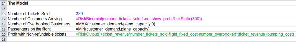
85 Airline Overbooking Step 2: Identify the decision variables. In this case there is one, the number of tickets sold. Step 3: Determine the model output. This is the profit. Assume no-shows are not refunded. Develop an expression for the profit. Let X be the number of overbooked customers. This is a random variable. Let Y denote the number of tickets sold. This is a decision variable. The profit random variable conditioned on the value of Y is: p(x Y ) = 500 Y X ( ) 80000

86 Airline Overbooking The number of tickets sold (value of Y ) is contained in cell B16. We fix this. The number of overbooked customers (the value of X ) is in cell B18. It is calculated by =MAX(customer_demand - plane_capacity, 0)

87 Airline Overbooking 87

88 Airline Overbooking 88 Step 4: Run the simulation.

89 Airline Overbooking Step 5: Analyze the outputs. Let X be the random variable denoting the number of overbooked customers. Let f (X ) denote the profit function. Sample Exam Question: In this example, what is f(e(x))? Sample Exam Question: In this example, what is E(f(X))? You must understand the difference between E(f (X )) and f (E(X )). I just pounded very loudly on the blackboard! KEY CONCEPT: Even when E(f (X )) = f (E(X )) simulation is very useful. Why?

90 Airline Overbooking 90 Modification: Assume that tickets are refundable. How does this affect the profit calculation? Step 3: Determine the model output. This is the profit. Again, let X be the number overbooked customers. This is a random variable. Let Y denote the number of tickets sold. The profit random variable conditioned on the value of Y without refunds was p(x Y ) = 500 Y X ( ) With refunds the revenue is 500 min(y, 300) where 300 is the plane capacity. The new profit function is p(x Y ) = 500 min(y, 300) X ( )

91 Airline Overbooking 91 Run Simulation and Analyze Results: Non-refundable Refundable Mean Profit $84,276 $67,294 Minimum Profit $73,750 $57,000 Maximum Profit $85,000 $70,000 Std. Dev. $1,541 $1,990

92 Airline Overbooking 92 Optimization: Treat the number of tickets sold as a variable / adjustable cell and find the optimal number of tickets to sell. Consider values between 300 and 440 in increments of 10 tickets. Run simulations for both the non-refundable and refundable profit functions. Record the Mean, Min, Max, and Standard Deviation statistics for each run. Put the RiskSimTable in cell B16. This is the cell with the range name number tickets sold.

93 Airline Overbooking 93 We are running 15 simulations on Output Cells.

94 Simulation Basics 94 What is the optimal number of tickets to sell for the non-refundable profit function? What is the optimal number of tickets to sell for the refundable profit function?