36106 Managerial Decision Modeling Monte Carlo Simulation in Excel: Part I

Transcription

1 36106 Managerial Decision Modeling Monte Carlo Simulation in Excel: Part I Kipp Martin University of Chicago Booth School of Business November 1, 2017

2 Reading and Excel Files Reading: Powell and Baker: Chapter 14, See the Documentation and Examples folders in the Palisade RISK6 directory that was installed with your software. Files used in this lecture: retirement.xlsx retirementrisk.xlsx riskstatic.xlsx retirementriskgoal.xlsx

3 Learning Objectives 1. Understand why stochastic models are important 2. Understand the Flaw of Averages a truly critical concept for anyone working with spreadsheets perhaps the biggest takeaway of the quarter 3. Learn to run a basic Monte Carlo simulation learn how to replace a parameter with a distribution learn how to use simulation result statistical functions 4. Learn to Goal Seek

4 Lecture Outline Software Install Motivation The Flaw of Averages Simulation Basics Simulation Goal Seek Summary

5 5 Software Install DecisionTools Suite After installing the Precision Tools Suite: 1. Click on icon on your desktop 2. Use AddIns to on the Ribbon for future use.

6 Software Install DecisionTools Suite 6 From now on, you can open Excel and do not need to use the desktop icons. You should see Tab items for both PrecisionTree

7 7 Software Install DecisionTools Suite Tips: turn off extra CPU s close other apps minimize number of open workbooks

8 Software Install DecisionTools Suite 8 Tips: Mac User Setting for VM Ware

9 Where We Are Headed The natural progression of modeling: 1. Build a purely deterministic model all parameters known with certainty 2. Build a model (like Markowitz) where certain parameters are means and variances of a statistical distribution 3. Build a model where parameters are actually a random variable (a statistical distribution)

10 Where We Are Headed We are taking tools from earlier in the quarter and extending them to allow for stochastic parameters. Deterministic Tool Stochastic Tool Goal Goal Seek (Week 7) Data RiskSimtable (Week 8) Optimizer (Week 10) Important: Understand the difference between a deterministic model and stochastic model.

11 Motivation The Flaw of Averages Here is the key concept or big take away: If there are numbers in your spreadsheet that are not known with certainty, putting in estimated average values can lead to terrible results! we will enter distributions rather than numbers into cells. Consider the following retirement example:

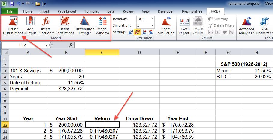
12 Motivation The Flaw of Averages 12 Assume a retirement 401 K account of $200,000 in the S&P. You want to withdraw equal amounts for the next 20 years until the fund is depleted. How much can you withdraw each year before hitting 0 at the end of year 20? Please open Workbook retirement.xlsx.

13 Motivation The Flaw of Averages In Workbook retirement.xlsx there are two spreadsheets: S&P 500: this spreadsheet has the S&P returns for This also has the calculations: 1. mean = standard deviation = model: this spreadsheet has the retirement calculations

14 Motivation The Flaw of Averages 14 A Few Things: 1. I am using the arithmetic mean not the geometric mean. 2. I am using annual compounding. 3. You may wish to use continuous compounding. 4. With continuous compounding, the arithmetic and geometric mean the same. 5. Using continuous does not affect the result I am demonstrating.

15 Motivation The Flaw of Averages Take a first cut using the PMT function in Excel. See cell B6, it has range name payment. There are five arguments: rate the interest rate to use in the calculation nper the number of payment periods pv the present value of your money, in this example the $200,000 at the beginning of the period fv the future value what you want to end up with after all the payments are made, in our case 0 type 0 if payments made at the end of the period, 1 if made at the beginning, the value is 0 if this argument is omitted

16 Motivation The Flaw of Averages 16 In this example we use the formula in cell named payment which is =PMT(interest_rate,years,-savings,0,1) and this translates to PMT(.1155, 20, , 0, 1) The value is $23, If you take out $23,327.72, while earning 11.55% on your money each year, you will drawn the account down to 0 at the end of 20 years.

17 17 Motivation The Flaw of Averages See the spreadsheet retirement.xls.

18 Motivation The Flaw of Averages See the spreadsheet retirement.xls. The key formulas are in columns B and E. For example, in cell B14 we have E13 This says that the amount of money at the start of year 3 is equal to the amount of money at the end of year 2. In cell E14 we have =IF(D14 > B14, 0, (1 + C14)*(B14-D14)) In the formula above we are saying that if the withdrawal amount is less than what we have in the account, the amount in the account at the end of the year is the beginning balance minus the withdrawal times (1 + return).

19 Motivation The Flaw of Averages In this analysis we assume that the S&P return is a constant 11.55% per year. But 11.55% per year is the average from Historically, the standard deviation over this period is 20.62% There is a serious problem with this!

20 Motivation The Flaw of Averages In the spreadsheet retirement.xls we make calculations based on the average interest rate. Everything is deterministic! In the spreadsheet retirementrisk.xls we use random interest rates with a mean of 11.55% and standard deviation of 20.62%. We simulate reality. Don t worry about how to generate random interest rates for now. First, let s look at some potential retirement scenarios. Then we will recreate retirementrisk.xls from retirement.xlsx.

21 21 Motivation The Flaw of Averages Argle Bargle!!! I am out of money after only five years! Handout anyone?

22 22 Motivation The Flaw of Averages What! Now I die with $561,151 left unspent. That is NOT fair!

23 23 Motivation The Flaw of Averages Argle Bargle!!! Out of money yet again.

24 Motivation The Flaw of Averages 24 Living a thousand lives. Distribution of years.

25 Motivation The Flaw of Averages 25 Living a thousand lives, cumulative probabilities.

26 Motivation The Flaw of Averages Sam Savage has a good explanation for what is going on. See his book the Flaw of Averages YouTube link

27 Motivation The Flaw of Averages This lecture is best summed up by the pictures on the following slides. The first picture was shamelessly stolen from the Web site of Sam Savage. But Sam is a nice guy and probably will not sue me. The second picture was from the San Jose Mercury Times. Hopefully they won t sue either.

28 Motivation The Flaw of Averages 28

29 Motivation The Flaw of Averages 29

30 Motivation The Flaw of Averages The bottom line the average can be pretty useless! A second rule of thumb: The more nonlinear the problem, the worse our results will be by using average values. Here is the problem: E(f (X )) f (E(X )) When you put average values into the cells (i.e. E(X )) you are calculating f (E(X )) but you really want E(f (X )). What is X in our retirement example? What is f (X ) in our case? Warning: f (X ) is a real ARGLE BARGLE!

31 Motivation The Flaw of Averages 31 In our case, f (X ) is COUNTIF(E12:E31,">0") and X corresponds to the values in C12:31. Not only is an IF involved, but we are counting IF statements! Pass me the defibrillator please!

32 32 Motivation The Flaw of Averages The Trace Precedents for f (X )!

33 Motivation The Flaw of Averages Here is a good example to help your intuition on why E(f (X )) f (E(X )) Consider a random variable X that can take on two values: the two values are X = 1 and X = 1 (the market is either up or down). Assume each event is equally likely and so the probabilities are: p(x = 1) =.5 and p(x = 1) =.5. The function of interest is: f (X ) = max(0, X ). What is f (E(X ))? What is E(f (X ))?

34 Motivation The Flaw of Averages What is f (E(X ))? E(X ) = = 0 f (E(X )) = f (0) = max(0, 0) = 0 What is E(f (X ))? E(f (X )) =.5 max(0, 1) +.5 max(0, 1) = =.5 E(f (X )) f (E(X ))

35 Motivation The Flaw of Averages Remember: A linear life is a good life. Some bad functions: IF MAX, MIN COUNTIF Before you took this course, you probably thought the IF function in Excel was pretty nice. Little did you know of the dangers that lurked below.

36 Simulation Basics Our goal is to replace parameters with distributions. We then sample from the distributions.

37 Simulation Basics In the following slides we take the workbook retirement.xlsx and create the content in workbook retirementrisk.xlsx. Step 1: use the Excel function COUNTIF. Put the formula =COUNTIF(E12:E31,">0") in cell E32. This will count the number of years where we end the year with a positive amount of money. Objective: run a 1000 trials and see the behavior of this number.

38 Simulation Basics Step 2 Incorporate Uncertainty: Here is how we incorporate uncertainty. We were using average values for the rates of return. This changes. In Column C, replace the fixed rates with random draws. Select Tab in the Ribbon. Select and clear the contents of cell C12. Select Cell C12 and then Define Distribution from the Model group. See next slide.

39 Simulation Basics 39

40 Simulation Basics 40 When you click on Define Distribution you will see: Select the Normal Distribution.

41 Simulation Basics 41 Put in the mean and standard deviation. Note the absolute addressing $H$3 and $H$4. We could have used the range names mean and std.

42 Simulation Basics We used Define Distributions to put in a distribution. Other options include: Use the Insert Function Just type it in (there is auto completion available)

43 Simulation Basics Step 3: Copy Cell C12 and paste it to Cells C13 to C31. Every time you recalculate the spreadsheet (F9 or recalculate under Formulas). We make a draw of a rate of return from the normal distribution with mean.1155 and standard deviation.2062 for cells C12 - C31. These draws are all independent of each other. That is, they are not correlated. More on this topic later. Make the font in cells C12 - C31 magenta. We are going to make our uncertain parameter cells magenta. I am open to other color selections.

44 Simulation Basics Step 4: Now, back to Cell E32. This is the cell we care about. It is telling how many years we end with a positive amount of money (a good thing). Key Idea: Cell E32 is really a random variable. Its value depends on other random variables. We care about the probability distribution of Cell E32! We to consider Cell E32 an output cell. See next slide.

45 Simulation Basics 45 Select Cell E32 and then click Add Output from the Model group.

46 Simulation Basics In Cell E32 you should see will now treat Cell E32 as a random variable and generate probability distribution information for the cell output.

47 Simulation Basics 47 Step 5: Run the simulation! My default is set for a 1000 trials. Don t worry about how many trials for now.

48 Simulation Basics 48 Step 5: Examine the output for Cell E32.

49 Simulation Basics 49 Here is the cumulative histogram.

50 Simulation Basics 50 How to stop the simulation. What to do if your simulation seems to be taking too long.

51 Simulation Basics 51 You can adjust the tails of the histogram by dragging or typing in the tail value you care about.

52 Simulation Basics 52 Other Hints: 1. The simulation will run much faster if you turn demo off. 2. I recommend you turn on Automatically Show Output Graph.

53 Simulation Basics Other Distributions: In Week 9 we will discuss more thoroughly selecting distributions for simulation. For now we consider two other distributions: (see riskstatic.xlsx) 1. RiskDiscrete 2. RiskUniform

54 Simulation Basics 54 Risk Discrete Distribution

55 Simulation Basics 55 Risk Uniform Distribution

56 Simulation Basics Sample Exam Question 1: In the retirement example, what is f(e(x)) when the payment is $23, and f(payment, returns) = COUNTIF(E12:E31,">0") Sample Exam Question 2: In this example, what is E(f(X)) when the payment is $23, and f(payment, returns) = COUNTIF(E12:E31,">0")

57 Simulation Basics The bottom line using averages can lead to bad results when the standard deviation is large! A rule of thumb: The greater the variance, the worse our results will be by using average values. The average high temperature for Chicago on April 1 is 53 degrees. Conclusion: If I wear a light jacket walking to the Harper Center I will be comfortable. The average high temperature for Honolulu on April 1 is 82 degrees. Conclusion: If I wear a tee shirt and jeans I will be comfortable.

58 Simulation Basics The bottom line using averages can lead to bad results when the standard deviation is large! Running Running Back 1 Back 2 Avg. yrds. per carry Std. Dev Situation 1: Own 20, ahead by 1 point, 5 minutes left in fourth quarter. Which back should carry? Situation 2: Own 20, down by 1 point, 5 minutes left in fourth quarter. Which back should carry?

59 Simulation Basics Summary: Using an expected value instead of a distribution is bad. Nonlinearity makes this even worse. Big standard deviations make this even worse.

60 Simulation Basics Color Coding: Black a parameter cell known with certainty (or at least treated as such) Magenta an uncertain parameter cell, one with distribution Blue an adjustable cell, a variable cell, something that we choose using Goal Seek or RiskSimtable() Green output cell (contains =RiskOutput() from Add Output)

61 Simulation Goal Seek 61 If we withdraw $23, per year, on average, it will last years. Not very satisfying. Even worse, there was a draw of only 3 years. Let turn the question around and see how much we can take out each year, and have a minimum draw of 18. there is a Goal Seek very similar to the Excel Goal Seek we used earlier in the quarter.

62 Simulation Goal Seek 62 The Goal cell is E32. This is the cell that counts the number of periods with a positive amount of money. We are interested in recording the minimum number of years for this cell. We change cell B6 which is the amount of money we withdraw each year.

63 Simulation Goal Seek 63 Notice we are restricting our search to be between 0 dollars and dollars.

64 Simulation Goal Seek 64 We should withdraw $4, Notice we did only 500 iterations per simulation. This should probably be larger.

65 Simulation Goal Seek Note: If you did not invest in the market, and got a 0 percent rate of return each year, you could withdraw $10,000 a year and die with zero dollars left. This suggests running a more complicated simulation where you can allocate your money between the stock market and a less risky asset.

66 Summary 66 Running a simulation creates a histogram for each cell in the spreadsheet that contains a RiskOutput(). You can put the summary statistics from the simulation directly in the spreadsheet.

67 Summary 67 You can insert functions with Insert Function, Statistic Functions, then Simulation Result.

68 Summary See the workbook retirementrisk. 1. In cell E33 I have inserted =RiskMean(E32,1). 2. In cell E34 I have inserted =RiskVariance(E32,1). After running a new simulation, these cells will hold, respectively, the simulation sample mean and variance. Cell E32 is the output of the simulation, it is =RiskOutput()+COUNTIF(E12:E31,">0").

69 Summary What we are doing is called Monte Carlo Simulation. The process was developed by Stanislaw Ulam and Nicholas Metropolis. Process developed while working on nuclear weapons projects at Los Alamos. Named after Monte Carlo where Ulam s uncle often gambled. Building a Monte Carlo Simulation Model: 1. Identify model inputs: deterministic inputs (black cells) random inputs (magenta cells) must also determine the distribution 2. Identify decision variable or variables (blue cells) 3. Identify model outputs (green cells) 4. Run the simulation 5. Analyze the outputs

70 Summary The benefit of Monte Carlo simulation Booth Students winning the 2012 SABR (Society for American Baseball Research) Competition. One of the things that distinguished the Booth (presentation) was their outstanding use of risk analysis, particularly their Monte Carlo simulations on playoff probabilities and (looking at) some of the other considerations that weighed into their decision, Gennaro (society president) said.

71 Summary Deja Vu all over again. Sample Exam Question: In this example, what is f(e(x))? Sample Exam Question: In this example, what is E(f(X))? You must understand the difference between E(f (X )) and f (E(X )). KEY CONCEPT: Even when E(f (X )) = f (E(X )) simulation is very useful. Why?