Credit Shocks in an Economy with Heterogeneous Firms and Default

Transcription

1 Credit Shocks in an Economy with Heterogeneous Firms and Default Aubhik Khan The Ohio State University Tatsuro Senga The Ohio State University Julia K. Thomas The Ohio State University February 2014 ABSTRACT We study aggregate fluctuations in an economy where firms have persistent differences in total factor productivities, capital and debt or financial assets. Investment is funded by retained earnings and non-contingent debt. Firms may default upon loans, and this risk leads to a unit cost of borrowing that rises with the level of debt and falls with the value of collateral. On average, larger firms, those with more collateral, have higher levels of investment than smaller firms with less collateral, causing an insuffi cient allocation of capital in small firms. Given the same distribution of productivity across large and small firms, this reduces aggregate total factor productivity, capital and GDP. We consider business cycles driven by exogenous changes in total factor productivity and by credit shocks. The latter are financial shocks that worsen borrowers cash on hand and reduce the fraction of collateral lenders can seize in the event of default. Our nonlinear loan rate schedules drive countercyclical default risk and exit. Because a negative productivity shock raises default probabilities, it leads to a modest reduction in the number of firms and a deterioration in the allocation of capital that amplifies the effect of the shock. The recession following a negative credit shock is qualitatively different from that following a productivity shock. A rise in default alongside a substantial fall in entry causes a large decline in the number of firms. Measured TFP falls for several periods, as does employment, investment and GDP. The recovery following a credit shock is gradual given slow recoveries in TFP, aggregate capital, and the measure of firms. Contact information: Aubhik Khan, mail@aubhik-khan.net; Tatsuro Senga, senga.1@osu.edu and Julia Thomas, mail@juliathomas.net.

2 1 Introduction Following the crisis in financial markets accompanying the 2007 recession in the U.S. and abroad, researchers have worked to better understand the extent to which the fall in real economic activity came in response to shocks originating in financial markets. We develop a quantitative dynamic stochastic general equilibrium model where shocks to financial intermediaries affect borrowers default risk and thus credit conditions facing nonfinancial firms, and thereby assess the relevance of such credit shocks for the recent economic downturn. Our approach is unique in having a distribution of firms over capital, debt and firm-specific productivity, endogenous firm entry and exit, and financial shocks that affect loan rate schedules offered to borrowers. Beneath the dramatic fall in aggregate lending and the sharp declines in aggregate investment and employment over the 2007 recession, disaggregated data reveals an unusual disparity in the impact on firms suggesting this recession may have been largely driven by a shock affecting firms ability to borrow. 1 Further, unlike most postwar recessions, this recent recession was characterized by declines in employment that were disproportionately concentrated among small firms. At the same time, the corporate sector as a whole held unusually large levels of cash at the start of the recession. 2 These observations suggest that a quantitative analysis of the real effect of a financial shock should include a nontrivial distribution of firms that vary in their capital, debt, and retained earnings. The model we develop contains all of these elements while, at the same, time, maintaining consistency with long-run macroeconomic data. We explore the extent to which financial shocks reducing the underlying value of collateral securing loans may have been responsible for the unusual reduction in lending volumes over the recent recession, the paths of real macroeconomic variables, and the disproportionate negative consequences among small firms and firms more reliant on external finance. We assume that firms may default on non-contingent debt. If a firm defaults, the lender recovers only a fraction of its capital. Thus, the interest rate charged on any given loan rises in the probability of default and it falls in the fraction of collateral recoverable under default. An unanticipated fall in this 1 Almeida et al (2009) find that firms that had to roll over a significant fraction of their debt in the year following August 2007 experienced a one-third fall in their investment relative to otherwise similar firms. 2 Using BED data originating from the Quarterly Census of Employment and Wages and maintained by the BLS, Khan and Thomas (2013) find that firms with fewer than one-hundred employees, as a whole, contracted employment by twice as much as large firms; see figure 8. Bates et al (2009) show that nonfinancial firms increased their cash holdings through See also Table C1 in Khan and Thomas (2013). 1

3 recovery rate serves as a credit shock in our model. In our model, competitive lenders choose loan rate schedules that provide them with an expected return for each loan equal to the real return on risk-free debt. As a firm s probability of default changes with its expected future productivity, capital stock and debt, its cost of borrowing is a function of its choice of debt and capital. By assuming that default deprives a firm of its assets and requires immediate exit, we derive several results that allow us to characterize borrowing and lending in general equilibrium. First, because we abstract from firm-level capital adjustment costs, we can show that idiosyncratic productivity and cash on hand are suffi cient to describe a firm s state. Second, we show that firm s values are continuous and weakly increasing in cash on hand. This implies the existence of threshold levels of cash on hand with which we can fully summarize firms decision rules regarding default. Specifically, given the current aggregate state, we derive threshold levels of net worth, which vary with idiosyncratic productivity, such that a firm repays its loan and continues operating only when its cash on hand exceeds the threshold associated with its current productivity. We exploit these results to numerically characterize borrowing and lending in a model where the aggregate state includes a distribution of firms over idiosyncratic productivity, capital and debt. In general, firms with higher expected future earnings or capital have a lower risk of default. This allows them to borrow more, and at lower cost. Thus, our borrowing limits are forwardlooking. By contrast, the risk of default rises with the size of the debt taken on. Beyond some level of debt, that risk becomes certainty, and there is no interest rate at which such a loan will be conveyed. Thus, each firm s ability to borrow is endogenously limited, and these borrowing limits vary across firms as functions of their individual state. We calibrate our model using firm-level investment and financial data, data on default rates, real aggregate data, and data from the flow of funds. We show that, in the long-run, borrowing and lending with non-contingent debt leads to a substantial misallocation of resources relative to a setting without financial frictions. Larger firms, those with more collateral, have higher levels of investment than smaller firms with less collateral. Considering that our firms all draw from the same persistent productivity distribution, the implication of this is that small firms in the economy have an ineffi ciently low allocation of capital and production. This misallocation, alongside endogenous exit in the event of default, reduces average aggregate total factor productivity, as well as GDP and capital. 2

4 When this model is driven by exogenous shocks to aggregate total factor productivity, noncontingent loans drive countercyclical default. Because a negative productivity shock raises default probabilities, it worsens the allocation of capital, thereby amplifying the effects of the shock. Measured aggregate productivity falls more than does the exogenous component of TFP, driving larger declines in production and investment. Thus, in contrast to previous findings by Kocherlakota (2000), Cordoba and Ripoll (2004) and Khan and Thomas (2013) in settings with exogenous collateral constraints, we find that our financial frictions affect the economy s response to nonfinancial shocks. Nonetheless, a productivity shock selected to yield the observed decline in measured TFP over the 2007 recession falls far short of explaining the observed declines in GDP, investment and employment, the reduction in lending is an order of magnitude too low and it does not yield disproportionate employment declines among small firms. When we examine the response to a financial shock, the greatest declines in output, employment and investment do not occur at the onset. This difference with an exogenous productivity shock lies in the resulting allocative disturbance. A credit shock affects expected future aggregate total factor productivity through a reduction in the number of firms and a worsening in the allocation of resources across them, but it has no direct effect on current production. Nonetheless, a financial shock that worsens borrowers financial position and lenders ability to seize defaulting firms collateral can eventually increase the misallocation of capital suffi ciently to cause a large and protracted fall in real economic activity. Our results suggest that this type of shock is able to explain the 2007 recession well in several respects. First, it generates unusually steep declines in GDP, investment and employment, while simultaneously predicting a comparatively modest decline in measured TFP. Second, these declines are more concentrated among small firms than large firms. Third, the recovery following a credit shock is unusually gradual because of a pronounced reduction in the number of firms driven by large increases in exit and reductions in entry over the downturn. Given decreasing returns to scale at individual firms, the number of available production units is itself a valuable stock that affects measured aggregate total factor productivity. Until this stock recovers, the return on capital remains low. This slows the return in investment in comparison to the recovery following a real shock, causing weaker, more gradual, recoveries in production and employment. 3

5 1.1 Related Literature Several recent studies have begun exploring how shocks to financial markets affect aggregate fluctuations. A leading example is Jermann and Quadrini (2012), which examines a representative firm model wherein investment is financed with debt and equity, while costs of adjusting dividends prevent the avoidance of financial frictions. These frictions stem from limited enforceability of debt contracts, which gives rise to endogenous borrowing limits. If the firm chooses to default, the lender can only recover a fraction of its net worth, and shocks to the fraction the lender can confiscate alter the severity of borrowing limits. Because the firm s enforceability constraint always binds, a credit shock to that constraint causes large reductions in real economic activity. Beyond our emphasis on heterogeneity and equilibrium default, a notable difference in our setting is that financial frictions do not dampen the response of the aggregate economy to non-financial shocks. This may be useful in light of findings by Reinhart and Rogoff (2009) and Bianchi and Mendoza (2012) that large financial shocks are rare in postwar U.S. history. Khan and Thomas (2013) study a more ad-hoc financial friction in the form of collateralized borrowing limits. There, a credit shock is an unanticipated change in the fraction of their collateral firms can borrow against. When hit by such a shock, that model delivers a large, persistent recession with some similar features to the 2007 U.S. recession. Our current work departs from this study in three important ways. First, while capital serves as collateral in our model, our borrowing limits depend on firm-level and aggregate state variables and arise from endogenous forward-looking lending schedules. Second, given the complexity associated with solving for equilibrium loan schedules, we abstract from the real microeconomic frictions considered there. Third, our model generates endogenous movements in entry and exit rates, and these series exhibit cyclical properties consistent with the U.S. data (see Campbell (1998)). This is particularly important in generating more gradual recoveries in employment and investment following a shock affecting financial markets, and thus greater consistency with the post 2009Q2 U.S. experience. Buera and Moll (2013) also study a heterogenous agent model with borrowing subject to collateral constraints. In their setting, entrepreneurs have constant returns production, face i.i.d. productivity shocks and observe shock realizations a period in advance. As a result, the distribution in their model does not evolve gradually over time as in ours, and they find shocks to collateral constraints are isomorphic to shocks to aggregate total factor productivity. Shourideh 4

6 and Zetlin-Jones (2012) also study financial shocks in a model where heterogeneous firms face collateral constraints. Their model features two types of intermediate goods producers, publicly owned and privately owned. They argue that financial shocks are a promising source of aggregate fluctuations when there are strong linkages through intermediate goods trades across firms. The financial frictions we study arise from non-contingent loans that introduce equilibrium default into the model. This type of loan contract was first characterized by Eaton and Gersovitz (1981) in their study of international lending. Recent work by Aguiar and Gopinath (2006) and Arellano (2008) undertake quantitative analyses of sovereign debt, while Chatterjee et al (2008) study an environment with unsecured lending to households. There are, however, well known alternatives to assuming non-contingent loans. Cooley, Marimon and Quadrini (2004) study constrained-optimal dynamic contracts under limited enforceability. Elsewhere, a large literature examines agency costs as the source of financial frictions, but does not consider financial shocks as such. 3 Our emphasis on productivity dispersion, non-contingent debt and equilibrium default is shared by Arellano, Bai and Kehoe (2012), who explore the extent to which aggregate fluctuations are explained by movements in the labor wedge driven by uncertainty shocks. Our study differs in that we include investment and study aggregate responses to financial shocks, our employment levels are not predetermined, and measured TFP is procyclical. 4 Our firms accumulate capital and may borrow or save. They have a natural maturing phase and tend to eventually outgrow default risk. Thus, the incidence of a credit shock differs, and we can explore the extent to which small firms are disproportionately affected. Following such shocks, shifts in the distribution of capital drive movements in aggregate total factor productivity through misallocation. In this respect, our study is also related to Buera and Shin (2013), who show that collateral constraints can protract the transition path to economic development if capital is initially misallocated. 2 Model Our model economy has three types of agents: households, firms, and a perfectly competitive representative financial intermediary. Only firms are heterogeneous. They face persistent differ- 3 See Bernanke and Gertler (1989), Carlstrom and Fuerst (1997), and Bernanke, Gertler and Gilchrist (1999). 4 Gomes and Schmid (2010) develop a model with endogenous default where firms vary with respect to their leverage and study the implication for credit spreads. Credit spreads are also a focus of Gertler and Kiyotaki (2010), who study a model where such spreads are driven by agency problems arising with financial intermediaries. 5

7 ences in their individual total factor productivities. Furthermore, their only source of external finance is non-contingent one-period debt provided by the financial intermediary at loan rates determined by their individual characteristics. These two aspects of the model combine to yield substantial heterogeneity in production. 2.1 Production, credit and capital adjustment We assume a large number of firms, each able to produce a homogenous output using predetermined capital stock k and labor n, via an increasing and concave production function; y = zεf (k, n), where F (k, n) = k α n ν, with α > 0, ν > 0 and α + ν < 1. Here, z represents exogenous stochastic total factor productivity common across firms, while ε is a firm-specific counterpart. Pr (ε = ε j ε = ε i ) π ij We assume ε is a Markov chain, ε E {ε 1,..., ε Nε }, where 0, and N ε j=1 πε ij = 1 for each i = 1,..., N ε. Similarly, z {z 1,..., z Nz }, where Pr (z = z m z = z l ) π z lm 0, and N z m=1 πz lm = 1 for each l = 1,..., N z. At the opening of each period, a firm is identified by its predetermined stock of capital, k K R +, the level of debt it took on in the previous period, b B R, and its current idiosyncratic productivity level, ε {ε 1,..., ε Nε }. We summarize the distribution of firms over (k, b, ε) using the probability measure µ defined on the Borel algebra generated by the open subsets of the product space, K B E. In our model, firms financial resources and their cost of borrowing are affected by credit shocks. These are determined by changes in θ, where θ {θ 1,..., θ Nθ } with Pr { θ = θ s θ = θ r } π θ rs 0 and N θ s=1 πθ rs = 1 for each r = 1,..., N θ. Let s = (z, θ) be the joint stochastic process for the exogenous aggregate state with transition matrix π s derived from the Markov Chains {π z } and { π θ }. The bivariate process s has a support with N s = N z N θ values. The aggregate state of the economy is fully summarized by (s, µ), and the distribution of firms evolves over time according to a mapping, Γ, from the current aggregate state; µ = Γ (s, µ). The evolution of the firm distribution is determined in part by the actions of continuing firms and in part by entry and exit, as will be made clear below. No microeconomic frictions impede capital reallocation in our model, so any firm s individual state in a period can be effectively summarized by its cash on hand, x. Given real wage ω (s, µ) and capital depreciation rate δ, the cash on hand of a type (k, b, ε) firm that operates is: x(k, b, ε; s, µ) = y(k, ε; s, µ) ω (s, µ) n(k, ε; s, µ) + (1 δ)k b ξ 0 χ θ (s) ξ 1 (ε), 6

8 where y and n represent the firm s output and employment. The fixed cost of operation, ξ 0 + χ (s) ξ 1 (ε), must be paid for the firm to operate in this or any future period. A firm can avoid it only by permanently exiting the economy prior to production. If it exits, the firm avoids both its debt repayment and operating cost, but it forfeits current flow profits and its capital stock, and achieves a value of 0. The fixed cost has two components, a real resource cost and a financial cost. Both must be paid whenever the firm wishes to continue operation. The real cost is stateinvariant while the financial cost χ θ (s) ξ 1 (ε), which varies with firm s idiosyncratic productivity, is positive only when the indicator function χ θ (s) = 1. This is the case whenever θ in s = (z, θ) is associated with a credit shock. Otherwise χ θ (s) = 0. Because our interest is in understanding how imperfect credit markets shape the investment decisions taken by firms, we require that firms dividends must always be non-negative to prevent them using equity to circumvent frictions in debt markets. Similarly, we must prevent all firms growing so large that none ever faces a borrowing limit or a cost of borrowing exceeding the current risk-free interest rate. To do this, we impose some state-independent exit and entry in the model. In particular, we assume each firm faces a fixed probability, π d (0, 1), that it will be forced to exit the economy following production in any given period. Thus, if µ t is the number of firms operating in date t, then π d µ t firms will leave the economy between dates t and t + 1 due to an exit shock. To maintain the total number of firms in our economy near 1 on average, there is also exogenous entry. At the end of any period, µ 0 potential firms are born with (ε, k, b) drawn from a distribution that we will describe below. Each potential entrant becomes a new firm if it pays operating cost and start-up loan. 5 Given the aggregate state (s, µ) and its start-of-period individual state (k, b, ε), each firm takes a series of actions to maximize the expected discounted value of its current and future dividends. First, it chooses whether to exit or remain in operation. To remain, the firm must be prepared to pay the fixed operating cost ξ 0 χ θ (s) ξ 1 (ε) and repay its existing debt b. If a firm defaults on its debt, it must immediately exit the economy, forfeiting all its remaining revenues and capital. If a firm fails to pay its operating cost, it also must immediately exit and so will at the same time default on its debt. Second, conditional on operating, the firm chooses its current level of employment and production, pays its wage bill, and repays its existing debt. After current production, wage payments and debt repayment, but prior to investment, each operating firm 5 If a potential firm does not enter, it defaults on its loan and leaves the economy having neither entered nor exited. 7

9 learns whether it will be permitted to continue into the next period. 6 If the firm is forced to leave the economy by an exit shock, it takes on no new debt and sells its remaining capital, thus achieving value x, which is paid to its shareholders as it exits. A continuing firm, by contrast, chooses its investment, current dividends, and the level of debt with which it will enter the next period. Before turning to continuing firms end of period decisions, we first examine the choices among all firms operating in the current period. Each firm that pays its operating cost to produce chooses its employment to solve: π (k, ε; s, µ) = max n [zεk α n ν ω (s, µ) n] where z is given by its value in s = (z, θ). given by: The firm s optimal labor and production are independent of its existing debt, b, and n (k, ε; s, µ) = ( νzεk α ω (s, µ) y (k, ε; s, µ) = (εz) 1 1 ν which in turn imply its flow profits net of labor costs, ) 1 1 ν ( ν ω (s, µ) (1) ) ν 1 ν k α 1 ν, (2) π (k, ε; s, µ) = (1 ν) y (k, ε; s, µ). (3) These values are common to all firms of type (k, ε) that find it worthwhile to operate given their start of period state (k, b, ε). At the end of the period, conditional on it producing, repaying its debt, and escaping the exit shock, a firm determines its future capital, k, future debt, b, alongside current dividends, D. Given investment, i, the firm s capital stock for the start of next period is determined by: k = (1 δ) k + i, (4) where δ (0, 1) is the rate of capital depreciation, and primes indicate one-period-ahead values. For each unit of debt it incurs for the next period, the firm receives q( ) units of output for use toward investment or current dividends. Thus a loan of q( )b implies debt of b to be repaid in the next period, and the continuing firm s current dividends are D( ) = x k + q( )b, where x is its cash on hand including current profits and the value of nondepreciated capital, after loan repayment and the payment of the fixed operating cost: x = π (k, ε; s, µ) + (1 δ) k b ξ 0 χ θ (s) ξ 1 (ε). (5) 6 We have adopted this timing to ensure that no default arises from the exogenous exit shock in our model. All firms borrowing this period will be able to produce next period. 8

10 In contrast to models with exogenous collateral constraints, our default risk implies that the loan discount factor faced by a borrowing firm depends on that firm s chosen debt and capital and its current productivity. Given a level of debt, a firm s capital choice for next period affects the distribution of its earnings and thus the probability it will repay. 2.2 Cash on hand and firm values Firms selecting the same k and b will not all have the same income next period because there is uncertainty in the firm-specific component of total factor productivity, ε. Among firms with common (k, b ), those realizing high productivities may repay their loans, while those realizing low ones may default. of the firm s nondepreciated capital. If a firm defaults, the financial intermediary recovers a fraction, ρ (θ), firms that repay their debts will pay operating costs to produce. Because a defaulting firm forfeits all its assets, only those When a continuing firm with current idiosyncratic productivity ε chooses to take on a debt b, alongside a future capital stock k, that firm receives q (k, b, ε; s, µ) b units of output in the current period. The loan discount factor, q (k, b, ε; s, µ), is determined as a function of the firm s repayment probability. Competitive lending equates the financial intermediary s expected return on each of its loans to the risk-free real interest rate. Letting π s lm d m (s l, µ) be the price of an Arrow security that pays off if s 1 = s m, the risk-free real rate is q 0 (s l,µ) 1, where: q 0 (s l, µ) = N s m=1 π s lm d m (s l, µ). (6) Each firm s loan discount factor is bounded above by the risk-free factor, q 0 (s, µ), and below by 0. Given a chosen (k, b ), and given µ = Γ (s, µ), the firm will face q (k, b, ε; s, µ) < q 0 (s, µ) so long as there is some possible realization of (ε, s ) next period under which the firm will default on its b. Among firms selecting a common (k, b ), those realizing higher ε next period will be less likely to default, as will be clear below. process, q (k, b, ε; s, µ) (weakly) rises in ε. falls in its b. Thus, given persistence in the firm productivity For the same reasons, the firm s q rises in its k and Recall the definition of an operating firm s cash on hand, x, from (5) above. In considering the lending schedule each firm faces, it is useful to note that a firm s individual levels of k and b do not separately determine any of its choices beyond their effect in x. To see this, note that a firm s resource constraint (determined by the non-negativity constraint on dividends) may be 9

11 written as simply: x k + q ( k, b, ε; s, µ ) b 0, in the absence of any costs of capital adjustment. This means that the firm s feasible capital and debt combinations are given by the set Φ (x, ε; s, µ), where: Φ (x, ε; s, µ) = {( k, b ) K B x k + q ( k, b, ε; s, µ ) b 0 }. (7) Since x fully captures previous decisions influencing its current choice set, the firm s value is also a function only of x and ε, and does not depend separately upon k and b. This important result allows us to reduce the firm-level state vector, and thus the dimension of the value and default functions that characterize competitive equilibrium. Let V 0 (x, ε i ; s l, µ) represent the beginning of period value of a firm just before its default decision, and let V 1 (x, ε i ; s l, µ) represent its value conditional on repaying its debt and operating. If Φ (x, ε i ; s l, µ) { }, the firm can cover its operating cost and repay its debt while paying a non-negative current dividend. non-negative value V 1 (x, ε i ; s l, µ). economy with zero value. In that case, the firm operates in the current period, achieving a Otherwise, it defaults on its debt and immediately exits the { } V 0 (x, ε i ; s l, µ) = max V 1 (x, ε i ; s l, µ), 0. (8) Given the constraint set in (7), it is straightforward to show that a firm s value is increasing in its cash on hand, x, and in its productivity, ε. The firm s value of operating, V 1, must account for the possibility of receiving the exogenous exit shock after current production and thus being unable to continue into the next period. Recall that, with probability π d, the firm is forced to exit at the end of the period. In that case, it simply pays out its cash on hand as dividend as it exits. Otherwise, it moves to the next period with continuation value V 2 determined below. V 1 (x, ε i ; s l, µ) = π d x + (1 π d ) V 2 (x, ε i ; s l, µ) (9) Given the current aggregate state, and given µ = Γ (s l, µ), firms continuing to the next period solve the following problem. 10

12 [ V 2 (x, ε i ; s l, µ) = max x k + q ( k, b, ε i ; s l, µ ) b (10) k,b + N s m=1 π s lm d N ε m (s l, µ) π ε ijv 0 ( x jm, ε j ; s m, µ )], j=1 subject to : ( k, b ) Φ (x, ε i ; s l, µ) (11) x jm = π ( k, ε j ; s m, µ ) + (1 δ)k b ξ 0 χ θ (s) ξ 1 (ε j ), (12) where V 0 ( ) is defined in (8), Φ( ) is given by (7), and π( ) is from (3). 2.3 Loan rates We now turn to the determination of the loan discount factors, q( ). Let χ (x, ε ; s, µ ) be an indicator for a firm entering next period with cash on hand x and productivity ε, given aggregate state (s, µ ), with this indicator taking on the value 1 if the firm chooses to repay its debt, and 0 otherwise. Since V 1 is increasing in ε, it is possible to identify a threshold productivity, ε d (x ; s, µ ), at which the firm is indifferent to default, the ε d solving V 1 ( x, ε d ; s, µ ) = 0. The firm s probability of debt repayment, as of the start of the repayment period, is then simply its probability of drawing ε ε d (x ; s, µ ). This strategy can be adopted to identify firms default probabilities as of the end of the current period using the transition probabilities for s and ε. However, since s and ε are both Markov chains, it is more straightforward to express the determination of firms loan discount factors using threshold cash on hand values. Threshold cash values, x d (ε ; s, µ ) solve V 1 ( x d, ε ; s, µ ) = 0 and separate those firms of a given productivity level for which χ ( ) = 1 (those with x x d ) from those for which χ ( ) = 0 (those that default). Recall that the financial intermediary providing loans to firms is perfectly competitive. Thus, the interest rate it offers on any loan is determined by a zero expected profit condition. Taking into account the fact that the intermediary recovers no more than ρ (θ) fraction of a firm s remaining capital in the event of default (or b if that is smaller), and recalling the determination of x jm 11

13 from (12), we arrive at the following implicit solution for the loan discount factor. q ( k, b, ε i ; s l, µ ) b = N s m=1 π s lm d N ε m (s l, µ) j=1 π ε ij +[1 χ ( x jm, ε j ; s m, µ ) ] ] min{b, ρ (θ) (1 δ) k }, [ χ ( x jm, ε j ; s m, µ ) b (13) where x jm = π ( k, ε j ; s m, µ ) + (1 δ)k b ξ 0 χ (s) ξ 1 (ε j ). Note that the loan price determined by (13) gives the risk-neutral lender the same per-unit expected return as that associated with risk-free real discount factor, q 0 (s l, µ). If a loan involves ) no probability of default, then χ (x jm, ε j; s m, µ = 1 for every (ε j, s m ) with π ε ij > 0 and πs lm > 0. In that case, q (k, b, ε i ; s l, µ) b = N s m=1 πs lm d m (s l, µ) b, so q (k, b, ε i ; s l, µ) = q 0 (s l, µ). 2.4 Households We close the model with a unit measure of identical households Household wealth is held as one-period shares in firms, which we identify using the measure λ, and in one-period noncontingent bonds, φ. 7 Given the prices they receive for their current shares, m 0 (x, ε; s, µ), the risk-free bond price q 0 (s, µ) 1, and the real wage they receive for their labor effort, w (s, µ), households determine their current consumption, c, hours worked, n h, new bond holdings φ, and the numbers of new shares, λ (x, ε ), to purchase at ex-dividend prices m 1 (x, ε ; s, µ). The lifetime expected utility maximization problem of the representative household is: V h (λ, φ; s l, µ) = c + q 0 (s, µ)φ + [ ( max U c,n h,φ,λ c, 1 n h) + β subject to N s m=1 ( m 1 x, ε ; s l, µ ) λ ( d [ x ε ]) + and µ = Γ(s, µ). π s lm V h ( λ, φ ; s m, µ )] (14) [ ω (s l, µ) n h + φ ] m 0 (x, ε; s l, µ) λ (d [x ε]) Let C h (λ, φ; s, µ) and N h (λ, φ; s, µ) be the household decision rules for consumption and hours worked. Let Φ h (λ, φ; s, µ) describe the household decision rule for bonds, and let M h (x, ε, λ, φ; s, µ) be the quantity of shares purchased in firms that will begin next period with cash on hand x and productivity ε. 7 Households also have access to a complete set of state-contingent claims. As there is no household heterogeneity, these assets are in zero net supply in equilibrium; thus, for simplicity sake, we do not explicitly model them here. 12

14 3 Computing equilibrium In recursive competitive equilibrium, each firm solves the problem described by (8) - (12), households solve the problem described in (14), loans are priced according to (13), the markets for labor, output and firm shares clear, and the resulting individual decision rules for firms and households are consistent with the aggregate law of motion, Γ. Using C(s, µ) and N(s, µ) to describe the market-clearing values of household consumption and hours worked, it is straightforward to show that market-clearing requires that (a) the real wage equal the household marginal rate of substitution between leisure and consumption, (b) the risk-free bond price, q0 1, equals the expected gross real interest rate, and (c) firms state-contingent discount factors are consistent with the household marginal rate of substitution between consumption across states. q 0 (s, µ) = β ( ) ( ) w (s, µ) = D 2 U C(s, µ), 1 N(s, µ) /D 1 U C(s, µ), 1 N(s, µ) N s m=1 d m (s, µ) = βd 1 U ( ) ( ) π s lm D 1U C(s m, µ ), 1 N(s m, µ ) /D 1 U C(s, µ), 1 N(s, µ) ( ) ( ) C(s m, µ ), 1 N(s m, µ ) /D 1 U C(s, µ), 1 N(s, µ). We compute equilibrium in our economy by combining the firm-level profit maximization problem with the equilibrium implications of household utility maximization listed above, effectively subsuming households decisions into the problems faced by firms. Without loss of generality, we assign p(s, µ) as an output price at which firms value current dividends and payments and correspondingly assume that firms discount their future values by the household subjective discount factor. Given this alternative means of expressing firms discounting, the following three conditions ensure all markets clear in our economy. ( ) p (s, µ) = D 1 U C(s, µ), 1 N(s, µ) (15) ( ) ω (s, µ) = D 2 U C(s, µ), 1 N(s, µ) /p (s, µ) (16) q 0 (s, µ) = β N s m=1 π s lm p (s m, Γ (s, µ)) /p (s, µ) (17) We reformulate (8) - (12) here to obtain an equivalent, more convenient, representation of the firm problem with each firm s value measured in units of marginal utility, rather than output. { } v 0 (x, ε i ; s l, µ) = max v 1 (x, ε i ; s l, µ), 0. (18) 13

15 v 1 (x, ε i ; s l, µ) = π d xp (s l, µ) + (1 π d ) v 2 (x, ε i ; s l, µ) (19) [ v 2 (x, ε i ; s l, µ) = max [x k + q ( k, b, ε i ; s l, µ ) b ]p (s l, µ) (20) k,b +β N s N ε m=1 j=1 subject to : (11) and (12). π s lm πε ijv 0 ( x jm, ε j ; s m, µ )], The problem listed in equations (18) - (20) forms the basis for solving equilibrium allocations in our economy, so long as the prices p, ω and q 0 taken as given by all agents satisfy the restrictions in (15) - (17), and the loan price schedules offered to firms satisfy (13). As noted above, a firm of type (k, b, ε) hires labor and produces only if v 1 (x, ε; s, µ) 0, where x = π (k, ε; s, µ) + (1 δ)k b ξ 0 χ θ (s) ξ 1 (ε). In that case, its decision rules for labor and output are given by (1) - (2), and its flow profits are given by (3). The more challenging objects we must determine are D, k and b for firms continuing into the next period. These decisions are dynamic and inter-related, and they depend on firm productivity, ε, and cash on hand, x. To solve for the forward-looking decisions of continuing firms, we use a partitioning of firms analogous to that in Khan and Thomas (forthcoming), here extended for the fact that we study noncontingent debt with default and exit. In particular, we assign firms across three distinct categories reflecting the extent to which their investment activities can be affected by financial frictions and identify their decision rules accordingly. Firms termed unconstrained are those that have permanently outgrown the implications of financial frictions. Firms that are constrained type 1 can undertake effi cient investment in the current period while borrowing at the risk-free interest rate, but face the possibility of paying a risk premium in future. Constrained type 2 firms cannot finance effi cient investment this period without paying a risk premium. 3.1 Decisions among unconstrained firms An unconstrained firm has accumulated suffi cient cash on hand such that, in every foreseeable state, it will be able to finance its effi cient level of investment at the risk-free interest rate q 0. Because any such firm has effectively outgrown financial frictions, its marginal valuation on retained earnings equals the household marginal valuation of consumption, p, so it is indifferent between 14

16 financial savings and dividends. Viewed another way, the firm s value function is linear in its debt or financial savings, so b does not affect its k decision. Any such firm not forced by the exit shock to leave at the end of the period adopts the effi cient capital stock k (ε i ; s l, µ) solving (21) below, achieving value w 2 ( ), and, given its indifference to financing arrangements, it is content to adopt the debt policy B w ( ) we isolate below to maintain that indifference permanently. [ w 2 (x, ε i ; s l, µ) = max [x k + q 0 (s l, µ) b ]p (s l, µ) (21) k + β N s N ε m=1 j=1 π s lm πε ijw 0 ( x jm, ε j ; s m, µ )], where x jm is given by (12) and w0 (x, ε; s, µ) = p(s, µ)π d x + (1 π d )w 2 (x, ε; s, µ). We assign an unconstrained firm a minimum savings debt policy solving (22) - (23) to just ensure that it always maintains suffi cient wealth to implement its optimal investments with no default risk under all possible future paths of (ε, s). 8 Let B ( ) k, ε j ; s m, Γ (s, µ) define the maximum debt level at which a firm entering next period with k and realizing (ε j, s m ) will be unconstrained. This requires that the firm can adopt k (ε j ; s m, µ ) and B w (ε j ; s m, µ ) next period while maintaining D 0, and that it will choose to remain in the economy. The unconstrained firm debt policy, B w (ε i ; s l, µ), is the minimum B jm ; i.e., it is the maximum debt with which the firm can exit this period and be certain to be unconstrained next period, given that it adopts k (ε i ; s l, µ). ( ) B w (ε i ; s l, µ) = min B k (ε i ; s l, µ), ε j ; s m, Γ (s, µ), where (22) {ε j π ε ij >0 and s m π s lm >0} B(k, ε i ; s l, µ) π(k, ε i ; s l, µ) + (1 δ) k ξ 0 χ θ (s) ξ 1 (ε i ) (23) {[ ] } + min k (ε i ; s l, µ) + q 0 (s l, µ)b w (ε i ; s l, µ), x d (ε i ; s l, µ), and x d (ε i ; s l, µ) solves v 1 ( x d, ε i ; s l, µ ) = 0. debt, we retrieve unconstrained firms dividend payments as: Finally, given their decision rules for capital and D w (x, ε i ; s l, µ) = x k (ε i ; s l, µ) + q 0 (s l, µ)b w (ε i ; s l, µ). (24) 3.2 Decisions among constrained firms We now consider the decisions made by a firm that has not yet been identified as unconstrained. We begin by evaluating whether the firm has crossed the relevant wealth threshold to 8 We adopt this policy rather than an alternative minimizing currrent dividends so as to bound the financial savings of long-lived firms. 15

17 become unconstrained. This is verified from equation 24 using the unconstrained firm decision rules (21) - (23). If D w (x, ε; s, µ) > 0, the firm is unconstrained and those decision rules apply. If not, it is still constrained in that financial considerations may continue to influence its investment decisions now or in future, so its choice of capital and debt remain intertwined. Constrained firms of type 1 can invest to the effi cient capital k (ε i ; s l, µ) from (21) in the current period while ensuring that all possible resulting x jm for next period will imply zero ) probability of default; in other words, χ (x jm, ε j; s m, µ = 1 for all j, m such that π ε ij > 0 and π s lm > 0, where x jm is from (12). Such firms optimally adopt k (ε i ; s l, µ) and borrow at the risk-free rate. Because they are sure to remain in the economy throughout the next period, but have not permanently outgrown financial frictions, their shadow value of internal funds exceeds the household valuation on dividends. Thus, they set D = 0 and b = q 0 (s l, µ) 1 [k (ε i ; s l, µ) x]. For constrained firms that do not satisfy the type 1 check above, we know of no convenient way to separate the loan implied by a given k choice to distinctly identify the corresponding debt level, b. Unlike type 1 firms above, a type 2 constrained firm may not find D = 0 optimal; it may in fact achieve higher expected discounted value by paying dividends in the current period if it faces suffi ciently high probability that it will be forced to default and exit the economy with zero value at the start of the next period. Thus, we must isolate the k, b and D choices of any such firm by applying a pure grid-based method to the problem listed in (18) - (20). Through the presence of type 2 constrained firms, the financial frictions in our economy generate two types of misallocation reducing aggregate TFP. First, since these firms face q (ε i, s l, k, b, µ) < q 0 (s, µ) for k = k (ε i ; s l, µ), they are led to adopt ineffi ciently small capital stocks either because they cannot borrow to k or because they are unwilling to suffer the implied risk premium. Second, with their low cash on hand and poor financing terms, these firms may default on their loans and exit the economy. Given decreasing returns to scale, the loss of a production unit further distorts the allocation of aggregate capital away from the effi cient one. 4 Calibration We explore the firm-level and aggregate implications of borrowing constraints across a series of numerical exercises. We assume that the representative household s period utility is the result of indivisible labor (Rogerson (1988)): u(c, L) = log c + ϕl. The firm-level production 16

18 function is Cobb-Douglas: zεf (k, n) = zεk α n ν, and firm-specific productivity is derived from an autoregressive log-normal process, log ε = ρ ε log ε + η, with η N ( 0, σ 2 η). We set the length of a period to be one year. Our annual calibration allows us to be consistent with establishment-level investment data that determines our idiosyncratic shock process. This, in turn, determines the typical level of capital reallocation in our model. We determine the values of β, ν, δ, α, and ϕ as follows. First, we set the household discount factor, β, to imply an average real interest rate of 4 percent, consistent with recent findings by Gomme, Ravikumar and Rupert (2008). Next, the production parameter ν is set to yield an average labor share of income at 0.60 (Cooley and Prescott (1995)). The depreciation rate, δ, is taken to imply an average investment-to-capital ratio of roughly 0.069, which corresponds to the average value for the private capital stock between 1954 and 2002 in the U.S. Fixed Asset Tables, controlling for growth. Given this value, we determine capital s share, α, so that our model matches the average private capital-to-output ratio over the same period, at 2.3, and we set the parameter governing the preference for leisure, ϕ, to imply an average of one-third of available time is spent in market work. Exact aggregation obtains in a reference model without financial frictions. We use that reference model to estimate an exogenous stochastic process for aggregate productivity. begin by assuming the shock follows a mean zero AR(1) process in logs: log z = ρ z log z + η z ) with η z N (0, σ 2 ηz. Next, we estimate the values of ρ z and σ ηz from Solow residuals measured using NIPA data on US real GDP and private capital, together with the total employment hours series constructed by Prescott, Ueberfeldt, and Cociuba (2012) from CPS household survey data, over the years We discretize this exogenous stochastic process as a 3-state Markov Chain, N z = 3. In the description of the model above, the only exogenous aggregate stochastic process was z. We now allow an additional component of the exogenous aggregate state by introducing credit shocks. These shocks to θ are follow a 2-state Markov chain with realizations {θ 1, θ 2 } and transition matrix: Π θ = p 1 1 p 1 1 p 2 p 2 We associate θ 1 with ordinary credit conditions and θ 2 with a credit shock. In the transition matrix, p 1 is the probability of continuing in ordinary borrowing conditions, Pr{θ = θ 1 θ = θ 1 }, while 1 p 2 is the probability of escape from crisis conditions, Pr{θ = θ 1 θ = θ 2 }. We select. We 17

19 the parameters of the Π θ matrix using evidence on banking crises from Reinhart and Rogoff (2009). Their definition of a banking crisis includes episodes where bank runs lead to the closure or public takeover of financial institutions as well as those without bank runs where the closure, merging, takeover or government bailout of one important financial institution is followed by similar outcomes for others. They document 13 crises in the U.S. since 1800 and the share of years spent in crises at 13 percent, which together imply an average crisis duration of 2.09 years. Given our use of postwar targets to calibrate the remaining parameters of our model, the more appropriate statistics for our purposes are those from the period , wherein the U.S. has had two banking crises (the 1989 savings and loan crisis and the 2007 subprime lending crisis). 9 Unfortunately, it is not possible to determine the average length of a U.S. crisis from this sample period, without knowing the ending date of the most recent crisis. Given this diffi culty, alongside Reinhart and Rogoff s argument that the incidence and number of crises is similar across the extensive set of countries they consider, we focus instead on their data for advanced economies. The average number of banking crises across advanced economies over was 1.4, while the share of years spent in crisis was 7 percent. Combining these observations, we set p 1 = and 1 p 2 = so that the average duration of a credit crisis in our model is 3.2 years, and the economy spends 7 percent of time in the crisis state. We set ρ (θ 1 ) = 0.37, consistent with estimates of debt recovery rates under default in ordinary conditions. We assume that a credit shock involves a recovery rate of 0. Furthermore, we set ξ 1 (ε i ) = 0.02π (ε i, k ) where π (ε i, k ) is the steady state level of profits of type 0 unconstrained firm operating with the effi cient level of capital for ε i. This simply scales the operating financial cost to the level of production of unconstrained firms. This financial fixed cost must be paid only when θ = θ 2. As a purely financial cost that implies a reduction in the cash on hand of firms that is transferred to households. In contrast to the real resource cost, ξ 0, ξ 1 (ε i ) does not enter the real aggregate resource constraint. Further, we assume that all capital that is in firms that default, and is not recovered by lenders, is lump sum rebated to households. Thus there are no real resource costs of credit shocks. We assume that all entrants begin with a common level of idiosyncratic productivity that is just below the median productivity level, ε 8. This is a simple approach to avoiding selection 9 These observations are consistent with findings by Bianchi and Mendoza (2012); they document a frequency of financial crisis at 3 percent, consistent with three financial crisis in the U.S. over the past hundred years. (2010) estimates a crisis frequency of 3.6 percent across emerging economies since Mendoza 18

20 among entrants that leads to their average productivity exceeding that of incumbents. Potential entrants draw capital from a Pareto distribution with lower bound k 0 and curvature parameter κ 0. They share a common level of debt, b 0. This ensure a distribution of potential entrants amongst which those with higher levels of capital will enter. We set κ 0 = 3 and choose k 0 to ensure that actual entrants are roughly 14 percent the size of a typical incumbent firm. We calibrate our model to reproduce the average aggregate indebtedness of firms in the U.S. economy. Towards this, we select our remaining parameters, ξ 0 (real operating cost), π d (exogenous departure rate among producing firms), k 0 (lower bound for capital in new firms), κ 0 (the distribution parameter for capital in new firms), alongside ρ ε and σ 2 η ε (persistence and volatility of firm productivity shocks) to reproduce the following 6 empirical targets: (i) the average debt-toassets ratio of nonfarm nonfinancial businesses over in the Flow of Funds (0.372), (ii) an average one-year cumulative default rate of 2 percent (Standard and Poor s), (iii) an average size among entrants, relative to incumbent firms, of approximately 14 percent, (iv) average entry and exit rates of 10 percent, and two aspects of establishment-level investment data documented by Cooper and Haltiwanger (2006) based on a 17-year sample drawn from the Longitudinal Research Database. The data on firm-level invest we target are (v) the average mean investment rate (i/k) across establishments (0.122) and (vi) the average standard deviation of investment rates (0.337). Given these parameters, we set the measure of firms that may choose to enter the economy, each period, µ 0, to have a long-run average number of firms in production equal to 1. While our model has life-cycle aspects affecting firms investments, the Cooper and Haltiwanger (2006) dataset includes only large manufacturing establishments that remain in operation throughout their sample period, Thus, in undertaking this part of our calibration, we must select an appropriate model-generated sample for comparability with their sample. We examine a subset of financially unconstrained firms. After choosing ( ) ρ ε, σ ηε as explained above, we increase the number discrete support of the idiosyncratic shock process and assume ε 1 = 0. This occurs with probability 0.1 independently of last period s idiosyncratic productivity level. Overall, this results in a discretised shocks process with N ε = 16. The introduction of a zero productivity idiosyncratic shock level allows us to reproduce a realistic life-cycle where firms do not rapidly overcome their borrowing constraints and adopt effi cient levels of capital. There are alternatives to ensure a similar distribution of firms. One is to allow ξ 0 to be scaled with ε as we have ξ 1. We further assume that all entrants 19

21 begin with ε = ε 8 and an initial debt level of b = The assumption of a common productivity level for entrants that is just below that of incumbents ensures that selection does not imply that new firms, more likely to be financially constrained, are more productive than incumbents. We have also assumed a size of entering firms that is somewhat higher than the lowest values typically assumed. Our choice of relatively large entrants implies higher levels of cash on hand, across entrants, than otherwise. This biases down the aggregate effects of the costs of borrowing. TABLE 1. Parameter Values β ν δ α ϕ ρ z σ ηz k 0 κ 0 π d µ 0 ξ 0 ρ ε σ ηε Results In our model, collateral constraints arise endogenously, and these constraints are forwardlooking. Among any group of firms sharing common cash on hand, irrespective of their current capital stocks, a firm with higher productivity can borrow more (at a better rate) than one with lower productivity. Compared to a setting with exogenous borrowing constraints, this tends to reduce the misallocation of capital across continuing firms. Nonetheless, shocks to the productivity of financial intermediation can cause large reductions in real economic activity. This is in part because, in endogenizing firms borrowing limits, we have introduced endogenous procyclical entry and countercyclical exit, which themselves amplify the effects of shocks in our model. 5.1 Steady state The aggregate implications of financial frictions even in our model s steady-state are considerable. Relative to an otherwise identical economy with perfect credit markets, the allocation of capital is distorted as firms choice of future capital, conditional on their current productivity, is a function of their cash on hand. Absent any financial frictions, each firm with current productivity ε i would simply select k to equate the unit purchase price of investment to its expected discounted marginal return to capital, q 0 π ij [π k (k, ε j ) + 1 δ]. Thus, k would depend only j 20

22 upon ε i, and the coeffi cient of variation of firms capital choices, conditional on ε, would be 0. In our economy, there is wide variation in firms k (x, ε) choices for any ε. Across all firms, the coeffi cient of variation of capital ranges from 0.14, for firms with the highest level of ε, to 1.5 for firms with the median non-zero level. Across firms with positive current productivity, persistence in idiosyncratic productivity leads firms with higher current productivity to expect higher levels of future cash on hand for any choice of capital and debt. As cash on hand is lost if a firm defaults, this makes them unlikely to default. As a result, more are able to adopt levels closer to their effi cient level and there is less dispersion in the capital choices of such firms. However, examining this dispersion across all levels of idiosyncratic productivity, its weighted average (with weights determined by the invariant distribution of ε) is A second source of capital misallocation arises from the fact that endogenous exit among firms with low cash on hand eliminates valuable productive locations. In the long run, when compared to a model with the same number of firms but without financial frictions, that is otherwise identical, the aggregate effect of these two sources of misallocation is to reduce steady state capital by 9.2 percent, GDP by 4.5 percent and consumption by 3.6 percent. Figure 1 presents firms decision rules for capital and debt as a function of cash on hand if they pay the fixed operating cost and produce (measured along the front axis, rising from right to left) and current productivity (measured along the right axis, rising from front to back). At any given level of productivity, each panel reflects four regions of firms. The right-most area, which starts below x = for firms with lower levels of ε and just below 0 for firms with higher levels, represents levels of cash on hand at which firms cannot obtain funds to finance any positive investment. Looking slightly leftward, we come to a narrow region where both the choice of capital and debt rise with the level of cash on hand. In this region, type 2 firms have their investment activities curtailed by the loan rate schedules they face. Leftward still, once x has risen suffi ciently, capital choices no longer rise with cash on hand and debt falls. This is a region associated with the decisions of type 1 firms. They adopt the frictionless capital stocks corresponding to their productivities and begin drawing down their debt. As x grows suffi ciently large, these firms begin to save. Finally, in the left-most region, for cash on hand between 4.34 for the lowest positive level of ε and 4.68 for the highest, we have unconstrained firms. The capital and debt or savings levels adopted by this group of firms depends only on productivity. While not shown here, it will be clear from the discussion in section 3 that only these firms pay 21

23 dividends, and their dividends are linear in x. Figure 2 focuses more closely on the decision rules from the previous figure, showing just three productivity levels (ε 2, ε 8 and ε 15 ) plotted in distinct panels. The middle panel shows the capital, debt and dividends adopted by firms with productivity just below the median level, while the upper and lower panels represent lower and higher productivity, respectively. Consistent with our observations from the previous figure, firms cannot borrow or invest when their production time cash on hand is very low. This is associated with levels at or below the default threshold. This default threshold is falling in ε. Persistence in idiosyncratic productivity, and the fact that profit and thus cash on hand is increasing in ε, implies that firms with higher current ε have higher expected future value. This makes them less likely to default on any current loan. Moving to higher levels of x, in the middle panel we see type 2 firms at cash on hand levels between around and As mentioned above, these firms capital choices rise with cash on hand. Current x predicts x which a firm will lose if its defaults, it follows that firms with higher current x generally have a higher probability of repaying their loans. As a result, loan discount rates offered to firms in this region generally improve with their cash on hand, and the b and k choices rise in x. One interesting aspect of this region is that, for some levels of cash on hand, type 2 firms will gamble. Firms with very low cash on hand take on more debt, choosing a higher risk premium, than other firms with more cash. Finally, for x between and , we have type 1 constrained firms. These firms adopt the frictionless capital choice without paying any risk premium, they choose k (ε) and steadily draw down their debt as their cash on hand rises. Figure 3 overviews the salient aspects of our economy s stationary distribution. There, we present the distribution of firms over debt (rising from right to left along the front axis) and capital (rising from front to back along the left axis) across all levels of idiosyncratic productivity, as firms enter the current period. Each of three types of firms may be identified in this figure. There are 15 horizontal line segments, associated with a different levels of ε (firms with ε 1 = 0 expect the same future distribution of future productivity as those with ε 8 ). Each line segment features a constant level of capital corresponding to the effi cient choice for an ε, these range from to , and a range of debt. At the end of the horizontal line segments, at the lowest levels of debt (and highest levels of financial savings), are unconstrained firms. In the absence of changes to their ε, such firms maintain k (ε) and choose b by following the minimum savings policy from (22) - 22

24 (23), which maintains their minimum cash on hand next period above a threshold level to ensure that they never face a risk premium in financing their investment loans. The weighted average debt level among unconstrained firms is Moreover, savings is negatively correlated with current capital choice and productivity. Debt levels for unconstrained firms range from for firms with the lowest ε to for firms with the highest. Mean reversion in ε implies that firms with lower current levels of idiosyncratic productivity expect higher percent increases in their effi cient level of future capital. They maintain higher levels of savings in order to be able to adopt the effi cient capital stock, in the future, following an increase in ε. Firms with higher current ε have higher levels of current capital and thus future collateral. The minimum savings policy allows them to hold debt without a positive probability of a future risk premium. Firms with the same capital stock as unconstrained firms, but higher levels of debt or lower levels of savings, are type 1 firms. They fill each line segment below its right endpoint. As already mentioned, these firms have the same capital stocks as unconstrained firms with the same idiosyncratic productivity, but pay no dividends. Instead they steadily reduce their debt, making their way rightward along their respective ε segments until they are able to follow both the capital choice and the savings rule for a corresponding unconstrained firm with their ε. The long diagonal, beginning at (k, b) = (0, 0) and moving northwest to k = and b near 3.7 shows the distribution of type 2 constrained firms. These firms begin with low levels of capital and debt, and slowly increase both as their cash on hand grows. Conditional on survival, once these firms reach the capital stock associated with effi cient investment for their ε, they become type 1 firms. Type 2 firms produce with ineffi ciently low levels of capital. Moreover, notice that the set of type 2 firms (which varies in current ε) is identified by an approximately constant leverage ratio. As we will show below, this implies that type 2 firms tend to have very similar levels of cash on hand, although they differ substantially in their size. It is these firms that transmit our economy s financial market imperfections into large reductions in GDP, investment and consumption When we simulate a large cohort of firms in our model s steady state, we find similar growth in the typical firm s capital and employment in the early periods of its life as present in the Khan and Thomas (forthcoming) exogenous collateral constraint model. There are two differences here. First, firm growth is conditional on survival, and our model has endogenous exit. Exit rates fall with age in our model as they do in the micro-level data (Dunne, Roberts and Samuelson (1989)). Second, conditional on survival, our firms reach maturity faster than in the Khan and Thomas model. This comes partly from our lack of investment irreversibilities and partly from the selection effect associated with our endogenous entry and exit. 23

25 Figure 4 overviews the implications of this stationary distribution for beginning of period cash on hand levels, corresponding to x + ξ 0. Of course, a potential firm that starts the period with a given (ε, k, b) will actually achieve π (k, ε) + (1 δ)k b only if it pays ξ 0 and continues into production. Unconstrained firms produce with probability one. The minimum level of cash on hand identifying an unconstrained firm is generally increasing in ε; as noted above, this ranges from 4.34 to 4.68, with a weighted average of At the other end of the figure, potential producers with levels of x near 0 are type 2. In between these two extremes are type 1 firms with higher levels of x, above the range , but below the thresholds for unconstrained firms. While many of the potential type 2 firms in the figure are new and will not choose to produce, and some are incumbent firms that will default on their debt and exit immediately, all type 1 and unconstrained firms continue into production and repay their debt. Thus, all exit by existing producers occurs among type 2 firms. As a result, across the distribution of potential firms at the start of a period shown in Figure 4, 7 percent are unconstrained, 53 percent are type 1 and 40 percent are type 2. However, only 36 percent of firms in production are of type 2, and they produce 12 percent of GDP. In sum, a small measure of firms in the economy actually produces with an ineffi ciently low capital stock 5.2 Business Cycles We now turn to a study of business cycles driven by both exogenous shocks to total factor productivity and credit shocks. We solve for stochastic equilibrium using the method of Krusell and Smith (1999). The endogenous component of the aggregate state is approximated using the first moment of the distribution of capital. Table 2 reports the results of a 5000 period simulation of the model. TABLE 2. Business Cycles with real and financial shocks x = Y C I N K r mean(x) σ x /σ Y (2.056) corr(x, Y ) Results are from a 5000 period simulation. The series reported are GDP, consumption, investment, total hours, capital and the real interest rate. All series are HP-filtered using a weight of

26 Credit shocks are relatively rare, and business cycles are largely driven by shocks to total factor productivity. The response of the economy with a rich distribution of firms broadly resembles a typical equilibrium business cycle model. GDP is more variable than consumption, investment is more variable than output and both are highly procyclical. When compared to a benchmark representative firm model, with no financial frictions, and the same production technology, the variability of GDP is slightly higher and its correlation with consumption and employment reduced. Figures 5 and 6 show our model s impulse responses following a persistent exogenous shock to the aggregate component of total factor productivity. We choose the size of the shock, 1.63 percent to result in a fall in measured aggregate TFP of approximately the same magnitude as observed in the 2007 U.S. recession (see below). In most qualitative respects, the economy s response is similar to that of a representative firm equilibrium business cycle model without financial frictions. The largest response is in investment, and the response in GDP exceeds that of consumption. Total hours worked, consumption and investment are procyclical. The responses in output, hours and investment are essentially monotone, and consumption exhibits the customary hump in its response. One notable aspect of Figure 5 is that measured total factor productivity (inferred from Solow residuals under the assumption of an aggregate production function in total capital and labor), falls further than does the exogenous component of TFP. Notice the gap between these two series in the bottom right panel; a 1.6 percent shock to TFP transmits to a 2.1 percent drop in measured TFP. This gap amplifies the initial declines in output, employment and investment somewhat, and, while narrowing over time, it persists for several periods. On balance, when the loan rate schedules facing individual firms are endogenous, we see that financial frictions do affect the economy s equilibrium response to an ordinary nonfinancial shock. This result is new relative to previous findings by Kocherlakota (2000), Cordoba and Ripoll (2004) and Khan and Thomas (forthcoming). Figure 6 may help explain this result. With the persistent decline in productivity, the risk-free real interest rate falls, implying a rise in the risk-free discount rate on loans seen in the top left panel. However, many firms cannot borrow at the risk-free rate, or cannot borrow what they wish to borrow. While not shown here, we know from our analysis in section 2.3 that the negative TFP shock leads to a general worsening of credit conditions for firms. Reduced productivity 25

27 necessarily generates rises in default probabilities. This, in turn, reduces firms ability to borrow, yielding a rise in the fraction of type 2 constrained firms, rationing their investment activities. With that said, the gradual decline in the overall level of debt in the economy is surprisingly similar to that observed in a model without financial frictions, or one with exogenous collateral constraints (Khan and Thomas (forthcoming)). What is new in our current environment is the set of results presented in the lower two panels of Figure 6. We noted above that the fall in aggregate productivity worsens credit conditions for firms. Given a reduced ability to borrow in light of reduced productivity, alongside reduced productivity on its own, firm values conditional on operating are reduced. Thus, the number of firms exiting the economy rises, and the number of entrants falls. Following the negative TFP shock examined here, the movements in entry and exit have nontrivial implications for the number of firms undertaking production. The number of producers initially falls by about 0.4 percent, and it continues falling over the next five years. By the start of period 6, the series is 0.9 percent below average. Given decreasing returns to scale at the firm (α + ν = 0.865), these changes deliver a separate source of misallocation beyond that associated with constrained capital choices among a fixed set continuing firms. It is this extra source of propagation, changes in the measure of producers, that is responsible for the endogenous reduction in measured TFP seen in Figure 5, and the sharper declines in aggregate production, employment, and investment in comparison to models without default. We now explore the response in our economy to a financial shock that increases firms cost of borrowing and reduces their cash on hand. Allowing θ to change from θ 1 to θ 2, the fraction of collateral lenders may recover falls from 0.37 to 0 while borrowers experience financial costs, ξ 1, that reduce their cash on hand. Because loan rate schedules are influenced by ρ (θ) and x (as shown in section 2.3), this shock directly increases the credit frictions facing firms. However, the credit shock, which is unanticipated and assumed to last for 4 periods, has no direct real effect on the economy. All capital of firms that default, and exit, is lump-sum returned to households. Furthermore, the financial fixed costs that reduce firms balance sheets are a transfer from firms to households. Figures 7 and 8 display our economy s impulse responses to this shock. In date 1, there is a small rise in GDP, employment and investment, while consumption falls marginally. Despite the anticipated decline in measured TFP (bottom right panel), and thus in the return to investment, 26

28 the wealth effect is dominant in the aggregate consumption and labor series, which also transmits to raised investment. Aggregate productivity begins falling in date 2 in part because the tightening of credit shifts type 2 constrained firms capital stocks further than normal from the frictionless capitals associated with their individual productivities and increases the relative number of such firms. However, reductions in the numbers of producers are also an important contributing factor. As was the case in response to the aggregate productivity shock considered above, our economy generates procyclical entry and countercyclical exit in response to the financial shock. The number of firms that exit (default) remains rises slightly in the first date of the shock, as seen in the lower left panel of Figure 8. Although they have more diffi culty borrowing to finance their capital for the next period, firms already have their capital in place for date 1 (and no real shock affects their productivity). However the fall in their cash on hand, following the financial shock, implies exit by firms with very low levels of cash on hand. Similarly, the value of entry falls given higher operating costs and increased diffi culty in borrowing. This reduces entry sharply at date 1. These things together reduce the number of firms producing in date 2. Over the next four periods, the number of producers continues falling and ultimately reaches 9 percent below normal. The upper left panel of Figure 8 illustrates how exacerbated misallocation (of both forms) affects the return to saving over our credit-generated recession. With no direct disturbance to aggregate productivity, the financial shock alone pushes the risk-free discount rate upward by roughly 0.14 percentage points. Alternatively, the expected real interest rate falls about 14 basis points below normal over the first four dates of the shock. The gradual decline in the real interest rate is driven the increased misallocation discussed above. Interestingly, the overall fall in lending in the top right panel of Figure 8 (at roughly 7 percent) is smaller than that following a shock to collateral constraints in Khan and Thomas (2013). This is in large part explained by the forward-looking nature of the endogenous collateral constraints we study here. It is type 2 firms that are directly affected by our credit shock. As in the previous study, these firms are typically smaller, younger firms. However, our endogenous borrowing schedules spare some such firms, because lending rates are affected by firm characteristics other than their existing capital. Firms with high productivity can borrow at better rates than otherwise similar firms with low productivity in our setting, and they can borrow more than their counterparts in a setting where exogenous borrowing limits tighten. 27

29 Returning to Figure 7, note that economic conditions worsen steadily following date 1 until 5 periods despite the constant credit shock. GDP falls 3.3 percent by date 5 and the eventual reduction in aggregate capital is only slightly larger, 4.25 percent. Moreover, the recovery following this recession is slow. The credit shocks ends immediately in figure 5 but both TFP and GDP continue to fall. Furthermore, despite the smaller decline in measured TFP, the recovery in GDP is far more gradual than that following the TFP shock in figure 5. Comparing figures 6 and 8, we see that there is far more damage to the number of potential producers (due to much larger declines in entry and rises in exit) in response to the credit shock. Given a fixed number of potential entrants each period, this large destruction to the stock of firms is only very gradually reversed. That in turn eliminates the incentive for a rapid rebound in investment (fueled by a rapid rise in employment) to repair the physical capital stock, which would otherwise follow a credit shock, because it holds measured TFP below average for a long time. As such, the slow rebuilding of the stock of firms protracts the recoveries in employment, investment and GDP. 5.3 The recent recession Table 3 compares the peak-to-trough behavior of our model, in response to TFP and credit shocks, with that over the 2007 U.S. recession. The data row reports seasonally adjusted, HPfiltered real quarterly series and measures declines between 2007Q4 and 2009Q2. An exception to this is the debt entry, where we report the ultimate drop in the stock of real commercial and industrial loans, which came later. TABLE 3. Peak-to-trough declines: U.S recession and model GDP I N C T F P Debt Data Credit shock TFP shock The credit shock row of Table 3 reports the declines in our model in response to the credit shock. The decline for real series are reported for date 5 when most series begin to recover. Declines in consumption continue for several further periods as GDP recovers gradually while the rebuilding of the capital stock begins; that series ultimately reaches 1.81 percent below average of 28

30 date 1. As in the data, debt in the model falls more slowly than GDP, and we report its ultimate decline which occurs in date 8. Notice that, relative to the endogenous decline in measured TFP, the reductions in GDP, investment, employment and debt are disproportionate under the credit shock. This unusual aspect of our model s response to a credit shock response resembles that over the recent U.S. recession. In our model, it appears to arise from the strong disincentives for investment in both physical capital and firms when misallocation not only worsens, but is anticipated to worsen further over coming periods. The nonmonotone path of measured TFP (despite the monotone path of θ) itself happens as further generations of new firms are affected by tightened credit conditions and vulnerable incumbents are ultimately forced to exit. In response to the productivity shock, by contrast, our responses in GDP, investment and employment are monotone. Thus, in the TFP shock row, we report impact date results for all series except debt. Since debt falls negligibly at the date of the shock, we report the drop in that series over 4 periods. Our credit shock appears small relative to the TFP shock if one considers its real effect on aggregate productivity. While the fall in measured TFP is roughly the same in the TFP shock row as in the data, it is far smaller in the credit shock row. Nonetheless, the credit shock generates roughly 60 percent of the observed reduction in GDP and 91 percent of the fall in investment. The fall in debt following a credit shock is 28 percent of the change seen in the data. By contrast, the exogenous TFP shock delivers a smaller drop in GDP and cannot deliver any significant drop in debt. Moreover, the fall in employment under the credit shock in our model is more than twice that under an exogenous aggregate productivity shock, and thus is closer to what was observed over the 2007 U.S. recession, though still far short of that value. 6 Concluding remarks We have developed a model where the aggregate state includes a distribution of firms over idiosyncratic productivity, capital and debt. Firms are risky borrowers, and equilibrium loan rate schedules are consistent with each borrower s default risk. We associate default with exit, and find that, following a persistent shock to exogenous total factor productivity, our model economy s response is broadly similar to a representative firm equilibrium business cycle model without financial frictions. In contrast, while our economy is consistent with the average aggregate 29

31 debt-to-asset ratio in the U.S., and only a small percentage of firms have investment hindered by financial frictions ordinarily, a credit shock in the form of reduced recovery rates for lenders in the event of default generates a large and lasting recession. Our model s credit shock recession unravels through two sources of capital misallocation that grow over several periods after the onset of the shock. First, there is a gradual rise in the misallocation of capital across continuing firms as several subsequent cohorts of young firms with little cash but high expected future productivity encounter worsened borrowing terms. Second, there are large endogenous reductions in firm entry and increases in exit following the credit shock that sharply reduce the number of firms over the downturn. Because the number of production locations is itself a valuable input affecting the productivity of the aggregate stock of capital, this second misallocation effect compounds the first in moving the distribution of production further away from an effi cient distribution and reducing measured productivity. Furthermore, because this substantial damage to the stock of firms takes time to repair, our model delivers a more gradual rebuilding of the aggregate capital stock, and thus more gradual recoveries in employment and investment than would otherwise occur. Overall, the recovery in GDP, following a credit shock, is far more gradual than that seen after a shock to total factor productivity. 30

32 References [1] Aguiar, M. and Gopinath, G. (2006) Defaultable debt, interest rates and the current account, Journal of International Economics 69(1), [2] Almeida, H., M. Campello, B. Laranjeira, and S. Weisbenner (2011) Corporate Debt Maturity and the Real Effects of the 2007 Credit Crisis, Critical Finance Review 1, [3] Arellano, C. (2008) Default Risk and Income Fluctuations in Emerging Economies, American Economic Review 98(3), [4] Arellano, C., Y. Bai and P. Kehoe (2012) Financial Markets and Fluctuations in Uncertainty, Federal Reserve Bank of Minneapolis Staff Report 466. [5] Bates, T. W., K. M. Kahle and R. M. Stulz. (2009) Why Do U.S. Firms Hold So Much More Cash than They Used To? Journal of Finance LXIV(5): [6] Bernanke, B. and M. Gertler (1989) Agency Costs, Net Worth, and Business Fluctuations, American Economic Review 79, [7] Bernanke, B., M. Gertler and S. Gilchrist (1999) The financial accelerator in a quantitative business cycle framework, Chapter 21, pages , in J. B. Taylor and M. Woodford (eds.) Handbook of Macroeconomics, Volume 1, Part 3, Elsevier. [8] Bianchi, J. and E. G. Mendoza (2012) Overborrowing, Financial Crisis and Macro-prudential Policy, University of Maryland working paper. [9] Boz, E. and E. G. Mendoza (2012) Financial Innovation, the Discovery of Risk, and the U.S. Credit Crisis, University of Maryland working paper. [10] Buera, F. and Moll, B. (2013) Aggregate Implications of a Credit Crunch, Princeton University working paper. [11] Buera, F. and Shin, Y. (2013) Financial Frictions and the Persistence of History: A Quantitative Exploration, Journal of Political Economy 121, [12] Campbell, J. (1998) Entry, Exit, Embodied Technology, and Business Cycles, Review of Economic Dynamics 1:

33 [13] Carlstrom, C. T. and T. S. Fuerst (1997) Agency Costs, Net Worth, and Business Fluctuations: A Computable General Equilibrium Analysis, American Economic Review 87, [14] Chari, V.V. (2012) A Macroeconomist s Wish List of Financial Data [15] Chari, V. V., L. Christiano and P. J. Kehoe (2008) Facts and Myths about the Financial Crisis of 2008, Federal Reserve Bank of Minneapolis Working Paper 666. [16] Chatterjee, S., D. Corbae, M. Nakajima and J. V. Ríos-Rull (2007) A Quantitative Theory of Unsecured Consumer Credit with Risk of Default, Econometrica 75, [17] Cociuba, S. E., Prescott, E. C. and A. Ueberfeldt (2012) U.S. Hours and Productivity Behavior Using CPS Hours Worked Data: 1947-III to 2011 University of Western Ontario working paper. [18] Cooley, T. F., R. Marimon and V. Quadrini (2004) Aggregate Consequences of Limited Contract Enforceability Journal of Political Economy, 2004, vol. 112, no. 4, [19] Cooley, T. F., Prescott, E. C., Economic Growth and Business Cycles. in Frontiers of Business Cycle Research, Cooley, T. F. Editor, Princeton University Press. [20] Cooper, R. and J. C. Haltiwanger (2006) On the Nature of Capital Adjustment Costs, Review of Economic Studies 73, [21] Cordoba, J.C. and M. Ripoll (2004) Credit Cycles Redux International Economic Review 45, [22] Davis, S.J. and J.C. Haltiwanger (1992) Gross Job Creation, Gross Job Destruction, and Employment Reallocation, Quarterly Journal of Economics 107, [23] Dunne, T., M. Roberts, and L. Samuelson (1989): The Growth and Failure of US Manufacturing Plants, Quarterly Journal of Economics 94, [24] Eaton, J. and M. Gersovitz (1981) Debt with Potential Repudiation: A Theoretical and Empirical Analysis" Review of Economic Studies 48, [25] Gertler, M. and N. Kiyotaki (2010) Financial Intermediation and Credit Policy in Business Cycle Analysis prepared for The Handbook of Monetary Economics. 32

34 [26] Gomes, J. F. and L. Schmid (2010) Equilibrium Credit Spreads and the Macroeconomy Wharton School working paper. [27] Gomme, P., Ravikumar, B. and P. Rupert (2008), The Return to Capital and the Business Cycle, Concordia University Working Paper [28] Gourio, F. (2013) Credit Risk and Default Risk, American Economic Journal: Macroeconomics 53(3), [29] Hennessy, C. and T. Whited (2007) How Costly is External Financing? Evidence from a Structural Estimation, Journal of Finance 62(4), [30] Jermann, U. and V. Quadrini (2012) Macroeconomic Effects of Financial Shocks American Economic Review 102(2), [31] Khan, A. and J. K. Thomas (2013) Credit Shocks and Aggregate Fluctuations in an Economy with Production Heterogeneity, Journal of Political Economy 121(6), [32] Kocherlakota, N.R. (2000) Creating Business Cycles Through Credit Constraints Federal Reserve Bank of Minneapolis Quarterly Review 24, [33] Krusell, Per and Anthony A. Smith (1998) Income and Wealth Heterogeneity in the Macroeconomy Journal of Political Economy, 106(5), pages [34] Reinhart, C. M. and K. S. Rogoff (2009) This Time Is Diff erent: Eight Centuries of Financial Folly, Princeton University Press. [35] Prescott, E. C. (1986) Theory Ahead of Business Cycle Measurement, Federal Reserve Bank of Minneapolis Quarterly Review 10, [36] Rogerson, R. (1988) Indivisible Labor, Lotteries and Equilibrium, Journal of Monetary Economics 21, [37] Shourideh, A. and A. Zetlin-Jones (2012) External Financing and the Role of Financial Frictions over the Business Cycle: Measurement and Theory, working paper. 33

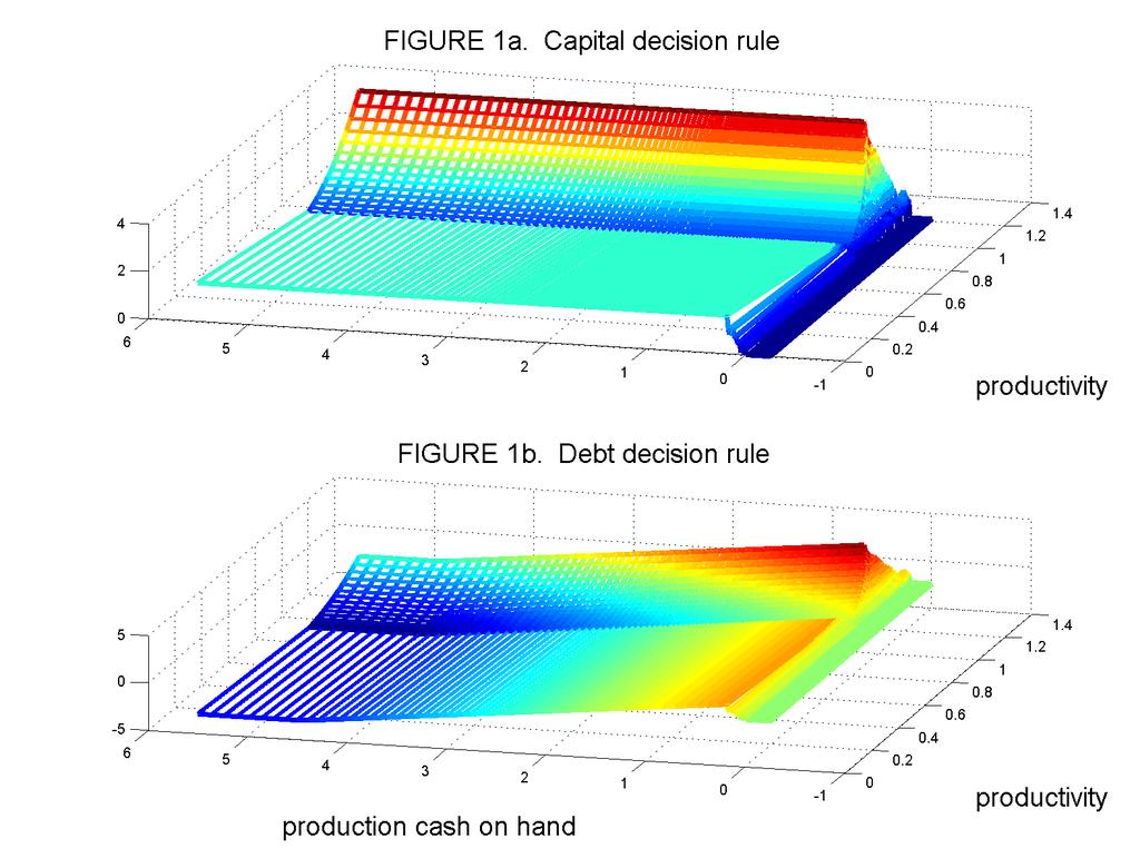
35