36106 Managerial Decision Modeling Monte Carlo Simulation in Excel: Part III

Transcription

1 36106 Managerial Decision Modeling Monte Carlo Simulation in Excel: Part III Kipp Martin University of Chicago Booth School of Business November 15, 2017

2 Reading and Excel Files 2 Reading: Powell and Baker: Chapter Simulation Elections Handout link for Week Nine. Files used in this lecture: distributions.xlsx confidence interval.xlsx markowitzcorrelation.xlsx markowitzcorrelation key.xlsx

3 Learning Objectives 1. Learn how to select among various probability distributions 2. Learn how to select a distribution based on data 3. Learn how to build a confidence interval on simulation outputs 4. Learn how to generate correlated random variables

4 Lecture Outline Motivation Probability Distributions Selecting a Distribution From Data How Many Trials? Correlation Stock Correlations Politics Blue or Red? St. Bernard Case Final Offer Arbitration

5 Errors 5 We would like to know E(f (X )) but there are pitfalls: 1. We must estimate f (X ) the function is just an estimate for reality 2. We must estimate X (the random variable) 3. We must run enough trials so that we can have confidence in f (X )

6 Probability Distributions THE KEY CONCEPT: Don t use averages, use distributions! A PROBLEM: if you use a woefully miscast distribution you may get bad results. A bad distribution may be worse than no distribution at all. maybe reality is very skewed and you use a symmetric distribution maybe outcomes are very correlated and you pick independent distributions First, address the problem of selecting a distribution. Then address the problem of correlated random variables.

7 Probability Distributions Some Options: If you have some historical data you could: 1. build a histogram and use RiskDiscrete (more on this later) 2. fit a distribution to your data (more on this later) 3. use your data to estimate certain parameters such as a mean and standard deviation and use these as inputs to a distribution (e.g. normal) If you do not have any data you could subjectively pick a distribution. In this case it important to understand which distribution might be most appropriate.

8 8 Probability Distributions (there are 71)

9 Probability Distributions Characteristics: Discrete versus Continuous Symmetric versus skewed (measure of asymmetry if you must know it is the third moment about the mean) Bounded versus unbounded Nonnegative versus positive and negative values

10 Probability Distributions Key Distributions: Discrete 1. RiskDiscrete ({x 1, x 2,..., x n}, {p 1, p 2,..., p n}) 2. RiskBinomial (N, p) 3. RiskBernoulli(p) 4. Poisson(Mean) Continuous 1. RiskUniform (Min, Max) 2. RiskTriang(Min, Most Likely, Max) 3. RiskPert(Min, Most Likely, Max) 4. RiskNormal(Mean, Std Dev) 5. RiskLognorm(Mean, Std Dev) 6. Exponential(Mean)

11 Probability Distributions RiskDiscrete ({x 1, x 2,..., x n }, {p 1, p 2,..., p n }): This is a discrete distribution that may be skewed. It is bounded and may have negative values. If you have historical data and make a histogram, you can use the histogram to produce a RiskDiscrete distribution. See distributions.xlsx

12 Probability Distributions RiskBinomial (N, p): where there are N trials and the probability of success is p. This is a discrete distribution that may be skewed. It is bounded and it is nonnegative. The mean of this distribution is pn. This applies when the trials are independent events, for example flipping a fair coin. You might use this as follows: you have sold 300 tickets for a flight. In the past the probability of a no-show is.1. The random variable for the number of people showing up is binomial with N = 300 and p =.9. See distributions.xlsx

13 Probability Distributions RiskBernoullil (p): The values of the random variable are either x = 1 with probability p, or 0 with probability 1 p. This is like the binomial when N = 1. This is a discrete distribution that may be skewed. It is bounded and it is nonnegative. We use this distribution is our simulation of election outcomes. See distributions.xlsx

14 Probability Distributions RiskUniform (Min, Max): Equally likely events in an interval. A continuous distribution A bounded distribution May assume positive or negative values See distributions.xlsx

15 Probability Distributions RiskPert (Min, Most Likely, Max) and RiskTriang (Min, Most Likely, Max): where Min is the minimum possible value, Max is the maximum possible value, and Most Likely, is well, most likely. Both are continuous distributions and may be asymmetric. They are bounded and may take on negative values. The Pert distribution put less emphasis on extreme values. See distributions.xlsx where the triangle and pert are superimposed. These are good distributions to use when: You want an asymmetric distribution (although Triangle and Pert can be symmetric). You do not have historical data, but have subjective guesses as to minimum, maximum, and most likely values.

16 Probability Distributions 16 The mean of the triangle distribution is (a + b + c)/3. All values weighted equally. The mean of the Pert distribution is (a + 4b + c)/6.

17 Probability Distributions RiskNormal(Mean, Std. Dev.): A continuous distribution that is symmetric. It is unbounded and may take on negative values. Good to use when Central Limit Theorem applies. Central Limit Theorem applies when you are summing independent random variables with well defined mean and variance.

18 Probability Distributions 18 RiskLognorm(Mean, Std. Dev.): A continuous distribution that is asymmetric. It is unbounded but does not take on negative or zero values. The lognormal random variable is given by X = e (µ+σz) where Z is a standard normal variable. For this random variable E(X ) = e (µ+σ2 /2) Var(X ) = (e σ2 1)e (2µ+σ2 )

19 Probability Distributions The lognormal is often used in finance to model stock prices. If you use continuous compounding and then take the log of the ratio of stock prices you get normally distributed returns. P t = P 0 e ( (r 0.5σ 2 )t+σt 0.5 Z) P 0 is the stock price at time 0 P t is the estimated stock price at time t r is the mean continuous compounding growth rate (estimate from data) σ is the continuous compounding growth rate standard deviation (estimate from data) Z is the Normal(0,1)

20 Probability Distributions 20 Using the expression for Expected value of the lognormal, one can show: E(P t ) = P 0 e rt See spreadsheet lognormal in the distributions.xlsx workbook. We estimate a stock price six periods out, two ways. 1. First way: generate values of N(0,1) and plug into the exponential formula P t = P 0 e ((r 0.5σ2 )t+σt 0.5 Z) 2. Second way: generate lognormal random values based on E(x) and Var(X ) where X = e ((r 0.5σ2 )t+σt 0.5 Z) P t = P 0 X

21 Probability Distributions 21 Simulate the stock price two ways.

22 22 Probability Distributions Result from using N(0,1) in exponential formula.

23 23 Probability Distributions Result from using lognormal distribution.

24 Probability Distributions Two important distributions often used in queuing (call centers, banks teller lines, etc.) are 1. Poisson model arrival rates (may lead to fishy results (ugh!)) 2. Exponential model service times

25 Probability Distributions You can even create your own. We did this for the Mergers and Acquisitions case. You can put them on a corporate SQL Server.

26 Selecting a Distribution From Data 26 You can to pick a distribution for you based on your data. It does a goodness of fit test based on the long laundry list of distributions supported Best of all, it is an easy process. We illustrate with the fitting spreadsheet in the distributions Workbook.

27 Selecting a Distribution From Data 27 The numbers in E3:E30 were generated by a normal distribution with mean 0 and standard deviation 10. This is what we are trying to fit below.

28 28 Selecting a Distribution From fits the normal distribution with a uniform with max and min

29 Selecting a Distribution From Data This example illustrates the difficulty of using a small sample size for fitting a distribution. Some sample sizes may not pick up the low probability events. In this sample, there were no realizations more than two standard deviations below the mean, and two standard deviations above the will often fit a non-symmetric triangular distribution to the normal sample data why do you think this might happen?

30 How Many Trials? 30 See the workbook confidence intervall.xlsx. Interval estimate of a population mean. s X ± t α/2 n X is the sample mean s is the sample standard deviation n is the sample size t α/2 is the t value for a (1 α) confidence interval with n 1 degrees of freedom (see next slide for appropriate Excel function)

31 How Many Trials? 31 Use Excel function T.INV.2T to calculate t α/2. See cell F32. It has the formula =T.INV.2T(alpha,$C32-1)

32 How Many Trials? 32 Consider the new product introduction model from Homework 6. The expected profit E(p(X, Y, Z)) is 7,100,000. We estimate this number through simulation. Simulation is nothing more than sampling. n Mean Std. Dev 95% Confidence Interval 10 7,084,302 2,473,681 7, 084, 302 ± , 473, 681/ ,135,080 2,617,859 7, 135, 080 ± , 617, 859/ ,102,757 2,468,202 7, 102, 757 ± , 468, 202/ ,100,207 2,466,928 7, 100, 207 ± , 466, 928/ 10000

33 How Many Trials? 33

34 34 How Many Trials? You can create a confidence interval using RiskCIMean(). =RiskCIMean(profit,0.9,FALSE,1)

35 Correlation 35 Consider the Workbook distributions.xlsx pictured below.

36 Correlation Objective: generate a scatter diagram. Here are the steps: Step 1: Insert a Risk Normal(0,10) in cell B8 and a Risk Uniform(-10,10) in cell B9. Step 2: Generate a histogram for Cell B9 which is the Risk Output for the Risk Uniform distribution. Step 3: Select a scatter plot. See next slide.

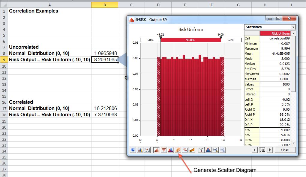
37 Correlation 37

38 Correlation 38 Step 4: Select Cell B8 with the Risk Normal as the second distribution for the scatter plot.

39 Correlation 39 Cell B8 is the output from a normal random variable with mean 0 and standard deviation 10. Cell B9 is the output from a uniform random variable with minimum value -10 and maximum value 10. These two random variables have zero correlation. A run of 1000 simulations gives the scatter plot below.

40 Correlation Important Takeaway: If you distributions in an Excel workbook, by default, they will have zero correlation. They will have a scatter diagram like on the previous slide. Zero correlation looks like a shotgun blast of bird shot. On the next slide we illustrate scatter diagrams for positive and zero correlation. For now, don t worry about how we generated these graphs.

41 41 Correlation A correlation of 0.8 between a normal and uniform random variable. Note the positive slope.

42 42 Correlation A correlation of -0.8 between a normal and uniform random variable. Note the negative slope.

43 43 Correlation Let X and Y be two random variables. The covariance between X and Y is cov(x, Y ) = E ((X µ X ) (Y µ Y )) = E ((X Y µ X Y X µ Y + µ X µ Y ) = E(X Y ) µ X E(Y ) E(X ) µ Y + E(µ X µ Y ) = E(X Y ) µ X µ Y µ X µ Y + µ X µ Y = E(X Y ) µ X µ Y Note: if X and Y have zero correlation, then and this implies E(X Y ) µ X µ Y = 0 E(X Y ) = µ X µ Y

44 Correlation 44 Let X and Y be two random variables. The correlation between X and Y scales the covariance to be between -1 and 1. ρ XY = cor(x, Y ) = cov(x, Y ) σ X σ Y = E ((X µ X ) (Y µ Y )) E ((X µx ) 2 ) E ((Y µ Y ) 2 ) Given sample means X and Y, that estimate µ X and µ Y, respectively, the sample correlation coefficient for X and Y is n i=1 (X i X )(Y i Y ) n i=1 (X i X ) 2 n i=1 (Y i Y ) 2

45 Correlation Okay math nerds, how does one generate correlated random variables? Here is the basic idea. 1. generate uncorrelated random variables 2. generate new random variables that are linear combinations of the uncorrelated random variables 3. the new random variables will be correlated and we find the right coefficients in the linear combination to give the desired correlations Here are some links with details: variables/ generate-correlated-normal-random-variables

46 Correlation you can generate correlated random variables. The user inputs the correlations using the RiskCorrmat function. There are two methods to specify correlations using RiskCorrmat. Regardless of which method you choose, you must first use Define Distributions to insert the random variables of interest.

47 Correlation Method One: Step 1: Decide which variables you think should be correlated. In our example, cells B17 and B18 contain the result of Define Distributions =RiskNormal(0,10) =RiskUniform(-10,10) Step 2: Generate a correlation matrix for these variables. The correlations typically come from historical data. I created a correlation matrix in the range correlationmatrix. Step 3: Manually edit cells B17 and B18 and insert the RiskCorrmat argument. Link the distributions back to the correlation matrix. See cells B17 and B18 with the edited formulas. =RiskNormal(0,10,RiskCorrmat(correlationMatrix,1)) =RiskUniform(-10,10,RiskCorrmat(correlationMatrix,2))

48 Correlation 48 Important: In the formulas below =RiskNormal(0,10,RiskCorrmat(correlationMatrix,1)) =RiskUniform(-10,10,RiskCorrmat(correlationMatrix,2)) it is important to link the random variable to the correlation matrix. This is what the 1 and 2 do, respectively.

49 Correlation Step 4: Run the simulation. Step 5: Look at the simulation output and create a scatter diagram. In the following slide I put -.8 into the correlation matrix. I added output to cell B18. I then treated cell B17 as the input. The scatter diagram plots the output versus the input.

50 Correlation 50 Note the sample correlation is

51 Correlation Method 2: Define Correlations. 51

52 Correlation 52 Select the random variables to correlate. Then type in the correlations.

53 Stock Correlations Creating correlated random variables is incredibly useful! Where we are headed: take the Markowitz model, and for a given portfolio, simulate returns based on the stock correlations.

54 Stock Correlations Open Workbook markowitzcorrelation.xlsx. In our the Markowitz optimization model there are three random variables: the monthly return on Apple stock denote by r X the monthly return on AMD stock denote by r Y the monthly return on Oracle stock denote by r Z There is a constraint on expected return. Let X denote the percentage of the portfolio invested in Apple, Y denote the percentage of the portfolio invested in AMD, and Z denote the percentage of the portfolio invested in Oracle. The unity constraint is X + Y + Z = 1.

55 Stock Correlations 55 The unity constraint is straightforward and does not involve random variables. However, the required return constraint does involve stochastic parameters (random variables). The required return constraint is E(r X X + r Y Y + r Z Z).12. We replaced this constraint with E(r X )X + E(r Y )Y + E(r Z )Z.12. Why is this a legitimate thing to do? What is f (r X, r Y, r Z )?

56 Stock Correlations 56 Here is the Markowitz optimal solution: X.12, Y = 0, and Z.88.

57 Stock Correlations The expected return of the portfolio is indeed, 12%. But what returns can we expect? Let s run a simulation of the portfolio based on the values of X =.12, Y = 0, and Z =.88. In order to do this, we must generate realizations of stock returns that are correlated! Let s examine the simulation model starting in row 21 of the spreadsheet markowitzcorrelation.xlsx.

58 Stock Correlations 58 Objective: Simulate portfolio returns.

59 Stock Correlations Step 1: Calculate the correlation matrix based on the sample returns using the formula below for each pair of random variables. n i=1 (X i X )(Y i Y ) n i=1 (X i X ) 2 n i=1 (Y i Y ) 2 Use the Excel function CORREL(Range1, Range2).

60 Stock Correlations 60 The returns for the three stocks are in the returns spreadsheet. For example, Cell D25 contains the correlation between Apple and Oracle. The formula is: =CORREL(apple_returns,orcl_returns) For example, Cell C27 contains the correlation between Oracle and AMD. The formula is: =CORREL(orcl_returns,amd_returns)

61 Stock Correlations Step 2: Now decide on the distribution for each of the random variables r X, r Y, and r Z. We took two approaches: Distribution Fitting to fit a distribution to the return data in the spreadsheet returns. This gives 1. For Apple the fitted distribution of returns is RiskUniform( , ) 2. For AMD the fitted distribution of returns is RiskUniform( ,1.2825) 3. For Oracle the fitted distribution of returns is RiskExtvalue( , ) See Row 34 Assume a normal distribution with mean and standard deviation set to the sample mean and standard deviation. See Row 35

62 Stock Correlations Step 3: Now add the RiskCorrmat function to each distribution. For example for the Apple fitted distribution we have =RiskUniform( , ,RiskName("AAPL"), RiskCorrmat(correlationMatrix,1,"fitted")) For the Oracle normal distribution we have =RiskNormal(orcl_mean,orcl_std_dev,RiskName("ORCL"), RiskCorrmat(correlationMatrix,3,"normal")) Important: we are using the same correlation matrix to generate the realizations for two distinct sets of random variables. Step 4: Run the simulation and look at the distribution of returns that are calculated in cells B38 and B39.

63 Stock Correlations 63 Argle Bargle! 45% of the time we experience a negative return for the fitted random variables! What percentage of the returns are below.12?

64 Stock Correlations 64 Argle Bargle! 38.7% of the time we experience a negative return for the normal random variables! What percentage of the returns are below.12?

65 Stock Correlations Next Week: 1. Use Risk Optimizer 2. Put a constraint on the fraction of time we can have negative returns.

66 Correlation in Senate Races Larry Robinson correlation example. See: 1. http: //faculty.chicagobooth.edu/kipp.martin/root/htmls/ coursework/36106/handouts/politics-correlation.pdf 2. risk-helps-zero-in-on-u-s-senate-race-outcomes/

67 St. Bernard Case 67 Please see corresponding Excel file stbernarddata.xlsx. This a capstone case combining many concepts used throughout the quarter. The theme of this case is that a municipal bond underwriter is submitting bids to a municipality.

68 St. Bernard Case 68 Step 1: The municipal bond underwriter makes a bid to the municipality of St. Bernard. This bid includes the following cash flows to St. Bernard. The face value of all the bonds that are going to be sold. In this case the total is $5 million. A premium which is the difference between the total coupon interest payments and the underwriter s profit (or spread). More on this later. Step 2: St. Bernard accepts or rejects the bid. Assume for now that they accept the bid of the underwriter in our case.

69 St. Bernard Case Step 3: Two weeks elapse and the underwriter sells the bonds in the marketplace. Assume all bonds are sold. For purposes of this case, the sole function of the underwriter is acting as a bond salesman for St. Bernard. The revenue to the underwriter is price of the bonds times the number sold. Hence the underwriter s profit is: bond sales revenue - 5,000,000 - premium Step 4: from the municipality pays the coupon rates on the bonds and the total face value of bonds (which is $5 million). The total cost to St. Bernard is then the face value of the bonds plus the coupon interest payments minus the premium they are paid. Hence they want total cost to be as small as possible and accept the bid that minimizes total cost.

70 St. Bernard Case 70 The sales price for the coupon rate - bond maturity

71 St. Bernard Case Understand: 1. yield curve 2. yield to maturity 3. coupon rate 4. face value 5. sales price

72 St. Bernard Case 72 An illustration of coupon rates assigned to maturities. Note the total revenue collected by the underwriter.

73 St. Bernard Case 73 For the given assignment, here are the interest payments by St. Bernard.

74 St. Bernard Case Here are the cash flows: 1. From underwriter to St. Bernard: $5,000,000 (face value of the bonds) premium = $5,148, $5,000,000 - $40,000 = $108, From investors to underwriter $5,148, (bond sales) 3. From St. Bernard to Investors $5,000,000 (bond face value at maturity) $1,162,625 (bond face interest payments)

75 St. Bernard Case 75 Objective: Minimize NIC (net interest charge) for St. Bernard in order to win the bid. For this example, the NIC is NIC = $1, 162, 625 $108, = $1, 053,

76 Final Offer Arbitration We know f (E(X )) is basically meaningless. 2. We can estimate E(f (X )) using simulation. However: E(f (X )) may be totally irrelevant, Basing a decision on E(f (X )) may lead to terrible results.