STA2601. Tutorial letter 105/2/2018. Applied Statistics II. Semester 2. Department of Statistics STA2601/105/2/2018 TRIAL EXAMINATION PAPER

Transcription

1 STA2601/105/2/2018 Tutorial letter 105/2/2018 Applied Statistics II STA2601 Semester 2 Department of Statistics TRIAL EXAMINATION PAPER Define tomorrow. university of south africa

2 Dear Student Congratulations if you obtained examination admission by submitting assignment 1. I would like to take the opportunity of wishing you well in the coming examinations. I hope you found the module stimulating. The examination Please note the following with regard to the examination: * The duration of the examination paper is two-hours. You will be able to complete the set paper in 2 hours, but there will be no time for dreaming or sitting on questions you are unsure about. Make sure that you take along a functional scientific calculator that you can operate with ease as it can save you some time. My advice to you would be to do those questions you find easy first; then go back to the ones that need more thinking. I do not mind to mark questions in whatever order you do them, just make sure that you number them clearly! * A copy of the list of formulae is attached to the trial examination paper. Please ensure that you know how to test the various hypotheses. * All the necessary statistical tables will be supplied (see the trial paper). * Pocket calculators are necessary for doing the calculations. * Working through (and understanding!) ALL the examples and exercises in the study guide, workbook and in the assignments as well as the trial paper will provide beneficial supplementary preparation. * Make sure that you know all the theory as well as the practical applications. * All the chapters in the study guide are equally important and don t try to spot! * Start preparing early and don t hesitate to call or me if something is unclear. The enclosed trial examination papers should give you a good indication of what to expect in the examination. Best wishes with your preparation for the examination and do not hesitate to contact me if you have any questions about STA2601. Ms S. Muchengetwa GJ GERWEL (C-Block), Floor 6, Office 6-05 Tel: (011) Cel: muches@unisa.ac.za 2

3 STA2601/105/2/2018 Trial paper 1 Reserve two hours for yourself and do the trial paper under exam conditions on your own! Duration: 2 hours 100 Marks INSTRUCTIONS 1. Answer ALL questions. 2. Marks will not be given for answers only. Show clearly how you solve each problem. 3. For all hypothesis-testing problems always give (i) the null and alternative hypothesis to be tested; (ii) the test statistic to be used; and (iii) the critical region for rejecting the null hypothesis. 4. Justify your answer completely if you make use of JMP output to answer a question. 3

4 May/June 2018 Paper One Final Examination QUESTION 1 (a) Name one distribution which is symmetric about zero. (1) (b) Complete the following: (i) The statistic T is called an unbiased estimator for the parameter θ if... (1) (ii) Let X 1,..., X n be a random sample from a population with unknown variance σ 2. An unbiased estimator for the population variance σ 2 is given by σ 2 =... (1) (c) Give, in general terms, the three main steps when calculating a maximum likelihood estimator for a parameter θ if the p.d.f. is f (X; θ). (Give formulae where appropriate.) (4) [7] QUESTION 2 (a) Let X 1, X 2 be independent random variables such that E(X 1 ) = c 1 θ 1 and E(X 2 ) = c 1 θ 1 + c 2 θ 2 where θ 1 and θ 2 are unknown parameters and c 1 and c 2 known constants. Find the least squares estimators for θ 1 and θ 2 (7) (b) Let X 1,..., X n be a random sample from a n(µ; σ 2 ) distribution. Let A 1 = 1 n n [ ] (n 1) (X i X) 2. Show that E(A 1 ) = σ 2. n i=1 (5) [12] 4

5 STA2601/105/2/2018 QUESTION 3 One hundred weaner lambs were weighed before being sent to market and the weights (in kilograms) grouped into the following table of observed frequencies: Class interval Observed frequency *Expected frequency (lamb mass) < > Note: The expected frequencies were computed under the assumption of a n (20; 4) distribution. The observed frequencies can be represented in a histogram as follows: Figure 1: Histogram of lamb weights (a) Does the histogram suggest that the sample originates from a normal distribution? Why (not)? (2) 5

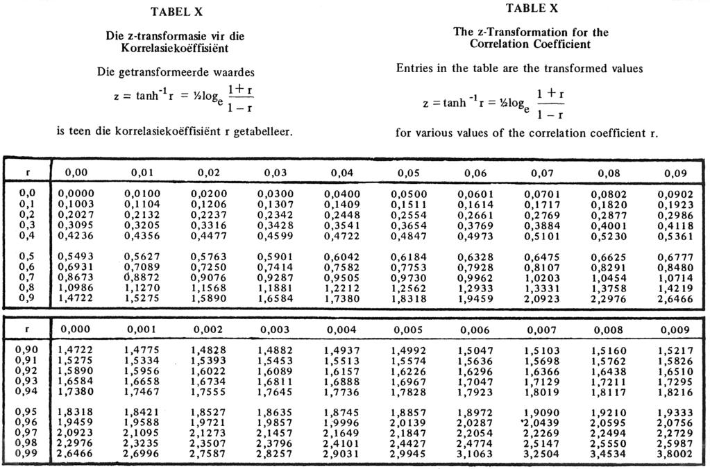
6 (b) Compute the chi-square goodness-of-fit statistic Y 2 to test whether the sample originates from a normal distribution with µ = 20 and σ 2 = 4. (6) (c) A statistical package computed the following statistics: x = 20 (x i x) 2 = (x i x) 3 = (x i x) 4 = Compute the statistics B 1 and B 2 as given in the formula sheet on page 8, as an alternative test for normality. Perform the two-sided tests for skewness and kurtosis at the 10% level of significance. (14) (d) Explain the differences (if any) between the conclusions of the two different tests for normality in (b) and (c). (3) [25] QUESTION 4 (a) A cell phone company conducts a survey in order to find out if awareness about 2 of its top selling cell phone models is equal among its customers based on a radom sample of n = 12 customers. The table below shows results obtained from the survey: Cell phone model Model 1 Model 2 Degree of awareness Yes No Test the hypothesis that the customers are equally aware of models 1 and 2 at the 0.05 level of significance (9) (b) In a random sample of 39 observations from a bivariate normal distribution, it was computed that r = 0.2 (i.e. the sample correlation coefficient). (i) Find a 95% confidence interval for ρ. (8) (ii) How can you use this confidence interval to test H 0 : ρ = 0 against H 1 : ρ 0 at the 5% level of significance? (2) [19] 6

7 STA2601/105/2/2018 QUESTION 5 The durability of tyres is tested by using a machine with a metallic device that wears down the tyres. The time it takes (in hours) for a tyre to blow is then recorded. "Safe Taxi" taxi company is trying to decide which brand of tyres to use for the coming year. Random samples from two different brands of tyres were drawn, the blowout times measured and the following statistics were computed from the data: Brand A N 1 = 25 Brand B N 2 = i=1 49 j=1 X i = 83 hours Y j = 196 hours 25 i=1 49 j=1 ( Xi X ) 2 = ( Y j Y ) 2 = (a) Do you think it is reasonable to assume that the two groups may be considered as independent groups? (2) (b) Use the 5% level of significance and test whether the variances of the two populations from which these samples were drawn, differ significantly. (9) (c) Test at the 5% level of significance whether the mean blowout time for tyres of Brand B is significantly higher than the mean blowout time for the tyres of Brand A. (Show how you interpolate for the critical value.) (7) (d) Comment on the assumptions that you have to make in order to perform the test in (c). (3) [21] 7

8 QUESTION 6 In order to determine the effect of a foliar-spray on the production of tomato plants, 12 tomato plants were sprayed with different doses of the foliar-spray. The following data were observed. Dose Yield x i y i (x i x) (x i x) 2 y i (x i x) Consider the simple linear regression model y i = β 0 + β 1 x i + ε i where the ε i s are independent n ( 0; σ 2) random variables. The following SAS JMP output is obtained. Figure 2a: The scatter plot 8

9 STA2601/105/2/2018 Figure 2a: The simple linear regression model (a) Show how the regression line of y on x is obtained and show all workings. (7) (b) Find a 95% confidence interval for the slope of the regression line computed in (a). (4) (c) What is the expected yield for x = 4? (1) (d) Find a 95% confidence interval for the expected yield of a new observation at x = 4. (4) [16] [100] 9

10 Trial paper 2 Reserve two hours for yourself and do the trial paper under exam conditions on your own! Duration: 2 hours 100 Marks INSTRUCTIONS 1. Answer ALL questions. 2. Marks will not be given for answers only. Show clearly how you solve each problem. 3. For all hypothesis-testing problems always give (i) the null and alternative hypothesis to be tested; (ii) the test statistic to be used; and (iii) the critical region for rejecting the null hypothesis. 4. Justify your answer completely if you make use of JMP output to answer a question. 10

11 STA2601/105/2/2018 May/June 2018 Paper Two Final Examination QUESTION 1 (a) Give the definition of an unbiased estimator. (1) (b) Explain what is meant by the significance level of a test (2) (c) Explain what is meant by the power of a test. (2) (d) Name two methods of obtaining point estimators. (2) (e) Name three methods of testing whether a sample comes from a normal distribution. (3) [10] QUESTION 2 Let X 1 ; X 2 ;... ; X n be independent random variables such that E(X i ) = θ 1, i = 1,..., (n 1) and E(X n ) = θ 1 + θ 2.. Find the least squares estimates of θ 1 and θ 2. [8] QUESTION 3 An aluminium company is experimenting with a new design for batteries. The main objective is to maximize the expected service life of a battery. Thirty batteries of the new design are tested and failed at the following ages (in days):

12 You may assume that n X i = i=1 n (X i X) 2 = i=1 n (X i X) 3 = i=1 We wish to test the null hypothesis that the observations come from a normal distribution by using a goodness-of-fit test. The 30 observed values were classified into the following six classes with equal probsability for each class interval. Equal probability intervals Expected frequency Count marks Observed frequency < X < X < X < X < X < X 5 5 Total 30 (a) State the null and alternative hypothesis. (2) (b) Under H 0 the distribution is not completely specified and we have to estimate the two unknown parameters by using the maximum likelihood estimators µ and σ 2 for the goodnessof-fit test. Calculate the values of the two unknown parameters. (5) (c) Show that the first interval is < X (4) 12

13 STA2601/105/2/2018 (d) Use the output in Figure 1 to make a conclusion on whether the data follows a normal distribution. Comment using all available information. Use α = Figure 1 (6) 13

14 (e) The following SAS JMP output was obtained: Figure 2 (i) Suppose that it is known that the standard (or the old ) design for the batteries has a mean service life of days. Can management conclude that the new design is superior to the standard design with respect to mean service life? (Test at the2.5% level of significance.) (4) (ii) Show that the 95% (two-sided) confidence interval for the mean service life, µ, of batteries of the new design is to (5) (iii) Show that the 95% two-sided confidence interval for the standard deviation (σ ) of the new design is to to (5) (iv) What assumptions do you make to do the confidence interval in (iii)? (1) [32] QUESTION 4 (a) In a summer tea-part in Pretoria, Pretoria, a lady claimed to be able to discern, by taste alone, whether a cup of tea with milk had the tea poured first or the milk poured first. An experiment was performed by a researcher to see if her claim is valid. Twelve cups of tea are prepared and presented to her in random order. Six had the milk poured first, and six had the tea poured first. The lady tasted each one and rendered her opinion. 14

15 STA2601/105/2/2018 The results are summarized in a 2 2 table below: Lady says Row Tea first Milk first total Poured Tea first Milk Column total Does the information above support the theory that the lady has no discerning ability? Test at the 5% level of significance. (9) (b) Fifteen patients with high blood pressure are chosen randomly and their blood pressure measured before, and two hours after, taking a certain drug. Patient Before (b) After (a) The following SAS JMP output was obtained: Figure 3 15

16 (i) Is this a matched pair or not? Explain. (1) (ii) Using the 0.05 level of significance, do the results confirm the drug company s claim that the drug lowers blood pressure? Clearly state the hypothesis implied by the question and how it can be tested. Give the rejection region and the conclusions. (5) (c) We wish to test H 0 : µ = 30 against H 1 : µ 30, using a sample of size n = 10. from a normal population with mean µ and variance σ 2. What is the power of the test if µ = σ? (4) (d) The scores obtained in maths (X i ) and stats (Y i ) by a random sample of n = 12 Year 1 UNISA students gave a sample correlation coefficient r 1 = Suppose that the same experiment is conducted on a random sample of n = 20 Year 2 UNISA students, and a correlation coefficient of r 2 = 0.89 is obtained. Test at the 1% level of significance the null hypothesis H 0 : ρ 1 = ρ 2 against the alternative hypothesis H 1 : ρ 1 < ρ 2. (6) [25] QUESTION 5 An agricultural experiment involving a control group and 3 experimental groups was performed to determine the effect of weed-killers on the yield of maize at a certain farm. A random sample of n = 32 plots with similar plot sizes and soil type are randomly assigned to 4 groups of 8 plots each. Group 1 was used as the control group, while Groups 2, 3 and 4 were used as experimental groups A, B and C in which weed-killers A, B and C were applied. The quantity of maize planted on each of the 32 plots was the same. The same amounts and types of fertilizer and irrigation methods were used on each plot. The following table shows the amount of yield in tons observed in each plot: Quantity of yield in tons Control Weed-killer A Weed-killer B Weed-killer C (X 1 ) (X 2 ) (X 3 ) (X 4 ) (Regard the data as random samples from normal populations.) 16

17 STA2601/105/2/2018 The following SAS JMP output was obtained. Figure 4 Figure 5 17

18 Figure 6 (a) Test at the 5% level of significance whether the population variances differ significantly from one another. (4) (b) Test at the 5% level of significance whether the population means of the four different groups differ. (i) State the null and alternative hypotheses. (ii) State the rejection region and conclusion. (4) 18

19 STA2601/105/2/2018 (c) Looking at output in Figure 6, can you conclude that µ 1 µ 2 = µ 3? Justify. (3) [11] QUESTION 6 A clinical trial consisting of a random sample of n = 20 cardiac patients is conducted in order to investigate the relationship between the dose given (X i ) and the number of cells killed (Y i ). The table below shows readings obtained from the clinical trial: Patient Dose given in Number of Dose given in Number of Patient cubic cms (X i ) dead cells (Y i ) cubic cms (X i ) dead cells (Y i ) The following output was obtained. Figure 7a 19

20 Figure 7b Assume that a linear relationship Y i = β 0 + β 1 x i + ε i where the ε i s are independent n ( 0; σ 2) random variables, is meaningful. Using Figure 4: (a) Does the assumption of linearity appear to be reasonable and why? (2) (b) Give the estimates β 0, β 1 and σ 2 for the model. (3) (c) What is the equation of the regression line used for the number of dead cells as a function of dose given? (1) (d) Predict the number of dead cells for 4 cubic cms of dose. (1) (e) At the 0.01 level, test the null hypothesis H 0 : β 1 = 0 versus H 1 : β 1 0. (4) (f) Find a 99% confidence interval for the slope of the regression line. (3) [14] [100] 20

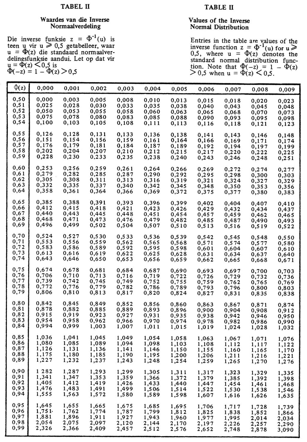
21 STA2601/105/2/2018 Formulae / Formules A= 1 n 1 n i=1 B 1 = n [ 1 n i=1 1 n i=1 B 2 = n [ 1 n i=1 1 n n i=1 n (X i X) 3 (X i X) 2 ] 3 2 n (X i X) 4 X i X n (X i X) 2 i=1 (X i X) 2 ] 2 ρ = eη e η e η + e η T = U 11 U 22 n 2 2 U 11 U 22 U12 2 T = (X 1 X 2 ) (µ 1 µ 2 ) S 1 n1 + 1 n2 υ = [ S 2 1 n 1 + S2 2 n 2 ] 2 S 4 1 n 2 1 (n 1 1) + S4 2 n 2 2 (n 2 1) F = k n k (X i X) 2 /(k 1) i=1 i=1 j=1 n (X i j X i ) 2 /(kn k) β 1 = n Y i (X i X) i=1 d 2 Note: d 2 = n (X i X) 2 and β 0 = i=1 n Y i β 1 i=1 n n X i i=1 = Y β 1 X 21

22 22

23 STA2601/105/2/

24 24

25 STA2601/105/2/

26 26

27 STA2601/105/2/

28 28

29 STA2601/105/2/

30 Table A. Percentage points for the distribution of B 1 Lower percentage point = (tabulated upper percentage point) Size of sample Percentage points Size of sample Percentage points n 5% n 5% 25 0, , , , , , , , , , , , , , , , , , , , , , , , , , , , , , , ,

31 STA2601/105/2/2018 Table B. Percentage points of the distribution of B 2 Size of Percentage points sample n Upper 5% Lower 5% 50 3, 99 2, , 87 2, , 77 2, , 71 2, , 65 2, , 57 2, , 52 2, , 47 2, , 44 2, , 41 2, , 39 2, , 37 2, , 35 2, , 34 2, , 33 2, , 31 2, , 29 2, , 28 2, , 26 2, 76 31

32 Table C. Percentage points for the distribution of A = mean deviation standard deviation Size of Percentage points sample n n 1 Upper 5% Upper 10% Lower 10% Lower 5% ,9073 0,8899 0,7409 0, ,8884 0,8733 0,7452 0, ,8768 0,8631 0,7495 0, ,8686 0,8570 0,7530 0, ,8625 0,8511 0,7559 0, ,8578 0,8468 0,7583 0, ,8540 0,8436 0,7604 0, ,8508 0,8409 0,7621 0, ,8481 0,8385 0,7636 0, ,8434 0,8349 0,7662 0, ,8403 0,8321 0,7683 0, ,8376 0,8298 0,7700 0, ,8353 0,8279 0,7714 0, ,8344 0,8264 0,7726 0,

33 STA2601/105/2/2018 Table D Tabel D The hypergeometric probability distribution: P (X x) for N = 12 Die hipergeometriese verdeling: P (X x) vir N = 12 n k x P n k x P n k x P , , , , , , , , , , , , , , , , , , , , , , , , , , , , , , , , , , , , , , , , , , , , , , , , , , , , , , , , , , , , , , , , , , , , , , , , , , , , ,000 33

34 Table E Upper 5% percentage points of the ratio, S 2 max /S2 min v k = , 0 87, , 4 27, 8 39, 2 50, 7 62, 0 4 9, 60 15, 5 20, 6 25, 2 29, 5 5 7, 15 10, 8 13, 7 16, 3 18, 7 6 5, 82 8, 38 10, 4 12, 1 13, 7 7 4, 99 6, 94 8, 44 9, 70 10, 8 8 4, 43 6, 00 7, 18 8, 12 9, , 03 5, 34 6, 31 7, 11 7, , 72 4, 85 5, 67 6, 34 6, , 28 4, 16 4, 79 5, 30 5, , 86 3, 54 4, 01 4, 37 4, , 46 2, 95 3, 29 3, 54 3, , 07 2, 40 2, 61 2, 78 2, , 67 1, 85 1, 96 2, 04 2, 11 1, 00 1, 00 1, 00 1, 00 1, 00 k = number of samples v = degrees of freedom for each sample variance 34

35 STA2601/105/2/2018 Table F: 100 (power) of the two-sided t-test with level α φ v = degrees of freedom α =

36 Table F (continued): 100 (power) of the two-sided t-test with level α φ v = degrees of freedom α =