MAT 4250: Lecture 1 Eric Chung

Transcription

1 1 MAT 4250: Lecture 1 Eric Chung

2 2Chapter 1: Impartial Combinatorial Games

3 3 Combinatorial games Combinatorial games are two-person games with perfect information and no chance moves, and with a win-or-lose outcome. Such a game is determined by a set of positions (including initial positions), and the players. Play moves from one position to another, with the players alternating moves, until a terminal position is reached. A terminal position is one from which no moves are possible. Then one player is declared the winner and the other the loser. Impartial games: the set of moves available from any given position is the same for both players. Partizan games: player has a different set of possible moves from a given position. We treat only impartial games.

4 A simple take-away game Rules for this simple impartial combinatorial game: 1. There are two players, labelled I and II. 2. There is a pile of 21 chips on the table. 3. A move consists of removing 1, 2 or 3 chips from the pile Players alternate moves with Player I starting. 5. The player that removes the last chip wins. Questions: How to analyze this game? Can one of the players force a win in this game? Which player would you rather be, the player who starts or the player who goes second? What is a good strategy? We use backward induction to analyze this game.

5 If there are just 1, 2 or 3 chips left, the next player wins. If there are 4 chips left, then the next player must leave 1, 2 or 3 chips and his opponent will win. Hence, 4 chips left is a loss for the next player and is a win for the previous player. 5 With 5, 6 or 7 chips left, the next player can win by moving to the position with 4 chips left. With 8 chips left, the next player to move must leave 5, 6 or 7 chips. So, the previous player wins. We see that 0, 4, 8, 12, 16, 20 are target positions, we would like to move into them. The first player wins by removing one chip and leave 20 chips.

6 Precise definition of combinatorial games Combinatorial game is a game that satisfies the conditions: 1. There are two players. 2. There is a finite set of possible positions The rules of the game specify for both players and each position which moves to other positions are legal moves. If the rules make no distinction between the players, the game is called impartial. Otherwise, the game is called partizan. 4. The players alternate moving. 5. The game ends when a position is reached from which no moves are possible. Under the normal play rule, the last player to move wins. 6. The game ends in a finite number of moves.

7 Remarks: 1. Under the misère play rule, the last player to move loses If a game never ends, it is declared a draw. We can always add an ending condition to eliminate this possibility. 3. No random move such as rolling of a dice is allowed. 4. A combinatorial game is a game with perfect information. Simultaneous moves and hidden moves are not allowed.

8 P-position and N-position Recall that, in the above take-away game, we see that 0, 4, 8, are positions that are winning for the Previous player and that 1, 2, 3, 5, are positions that are winning for the Next player. 8 0, 4, 8, are called P-positions and 1, 2, 3, 5, are called N-positions. P-positions are positions that are winning for the previous player and N-positions are positions that are winning for the next player. In impartial combinatorial games, one can find in principle which positions are P-positions and which are N-positions. We say a position is a terminal position if no moves from it are possible.

9 Finding P- and N-positions The method is very similar to the way we solve the take-away game. 1. Label every terminal position as a P-position. 2. Label every position that can reach a labelled P-position in one move as an N-position Find those positions whose only moves are to labelled N-positions. And label such positions as P-positions. 4. If no new P-positions were found in step 3, stop. Otherwise return to step 2. The strategy of moving to P-positions wins. From a P-position, your opponent can only move to N-position (3). Then you can move back to a P-position. Eventually the game ends at a terminal position (which is a P-position).

10 Characteristic property: (Under the normal play rule) P-positions and N-positions are define recursively by the following All terminal positions are P-positions. 2. From every N-position, there is at least one move to a P-position. 3. From every P-position, every move is to an N-position.

11 Subtraction games Consider a class of combinatorial games that contains the above take-away game. Let S be a set of positive integers. 11 The subtraction game with subtraction set S is played as follows. From a pile with a large number, say n, of chips, two players alternate moves. A move consists of removing s chips from the pile where s S. Last player to move wins. The above take-away game is a subtraction game with S = {1, 2, 3}.

12 An example: take S = {1, 3, 4}. There is exactly one terminal position, namely 0. Thus it is a P-position. Then 1, 3, 4 are N-positions, since they can move to must be a P-position because the only legal move from 2 is to 1. 5, 6 must be N-positions since they can be moved to 2. 7 must be a P-position since the only moves from 7 are to 6, 4, 3, which are N-positions. Similarly, 8, 10, 11 are N-positions, 9 is a P-position, 12, 13 are N-positions and 14 is a P-position.

13 Now repeat inductively, we see that P-positions are {0, 2, 7, 9, 14, 16, } and N-positions are {1, 3, 4, 5, 6, 8, 10, 11, 12, 13, 15, }. 13 x po P N P N N N N P N P N N N N Note that the pattern PNPNNNN of length repeats forever. Q: who wins the game with 100 chips, the first or the second player? The P-positions are the numbers equal to 0 or 2 modulus 7. Since 100 has remainder 2 when divided by 7, 100 is a P-position. Hence the second player will win with optimal play.

14 The game of Nim 14 The most famous take-away game is the game of Nim. There are 3 piles of chips containing x 1, x 2 and x 3 chips. Two players take turn moving. Each move consists of selecting one of the piles and removing chips from it. You cannot remove chips from more than one pile, but from the pile you selected you may remove as many as you want. The winner is the one who removes the last chip. You can play at

15 Preliminary analysis Exactly one terminal position (0, 0, 0), which is a P-position. 15 Any position with one pile, say (0, 0, x) with x > 0, is a N-position because you can win by removing all chips. Consider two non-empty piles. We see that the P-positions are those for which the two piles have an equal number of chips, e.g. (0, 1, 1). This is because your opponent must move to a position with an unequal number of chips, and then you can return to a position with equal number of chips. Consider all 3 piles are non-empty. Clearly (1, 1, 2), (1, 1, 3), (1, 2, 2) are N-positions because they can move to (1, 1, 0), (1, 1, 0), (0, 2, 2). Then we see that (1, 2, 3) is a P-position because it can only be moved to N-positions. How to generalize?

16 Nim-sum Every non-negative integer x has a unique base 2 representation of the form x = x m 2 m + x m 1 2 m x x 0 for some m, where each x i is either 0 or 1. We use (x m x m 1 x 1 x 0 ) 2 to denote this representation. 16 Ex: 22 = = (10110) 2. Definition: The nim-sum of (x m x 0 ) 2 and (y m y 0 ) 2 is (z m z 0 ) 2, and write (x m x 0 ) 2 (y m y 0 ) 2 = (z m z 0 ) 2 where z k = x k + y k (mod 2). It is the component-wise addition modulo 2 for the base 2 representation.

17 Example: = 37. Note that 22 = (010110) 2 and 51 = (110011) 2. Component-wise addition modulo 2 gives (100101) 2, which is 37. Remark: 17 Nim-sum is associative, i.e., x (y z) = (x y) z. Nim-sum is commutative, i.e., x y = y x. 0 is an identity, i.e., 0 x = x. Every number is its own negative, i.e., x x = 0. Cancellation law holds, i.e., if x y = x z, then y = z.

18 Question: what nim-sum have to do with playing the game of Nim? Theorem: A position, (x 1, x 2, x 3 ), in the game of Nim is a P-position if and only if the nim-sum of its components is zero, x 1 x 2 x 3 = Example: Consider the position (13, 12, 8). Is this a P-position? If not, what is a winning move? Note that 13 = (1101) 2, 12 = (1100) 2 and 8 = (1000) 2. The nim-sum is (1001) 2 = 9. Thus it is a N-position. How do we find a winning move? We need to find a move to a P-position. We need to move to a position such that there are even number of 1 in each component. Simply take away 9 chips from the first pile.

19 Proof of theorem: need to check the 3 conditions. Let P be the set of positions with nim-sum zero and N be the complement (with positive nim-sum) All terminal positions are in P. The only terminal position is (0, 0, 0), so it is in P. 2. From each position in N, there is a move to a position in P. Look at the leftmost component with odd number of 1. Change a number with 1 in that component so that there are even number of 1 in that component. You get a smaller number. Thus this is a legal move to a position in P. 3. Every move from a position in P is to a position in N. If (x 1, x 2, x 3 ) P and x 1 is changed to x 1 < x 1. Then the nim-sum of (x 1, x 2, x 3 ) cannot be zero. Otherwise, cancellation law implies that x 1 = x 1.

20 1 MAT 4250: Lecture 2 Eric Chung

21 Graph games 2 We give a description of combinatorial games as a game played on a directed graph. We identify the positions in a game with vertices of the graph and moves of the game with edges of the graph. Definition: A directed graph G is a pair (X, F) where X is a non-empty set of vertices (positions) and F is a function that gives for each x X a subset of X, F(x) X. Here F(x) represents the positions to which a player may move from x (also called the followers of x). If F(x) is empty, x is called a terminal position.

22 A two-person game may be played on such a graph G = (X, F) by choosing a starting position x 0 and using the following rules 1. Player I moves first, starting at x Players alternate moves. 3. At position x, the player can only move to positions y where y F(x) The player who is confronted with a terminal position loses. Remark: We assume that the graph is progressively bounded so that a terminal position is reached in a finite (and bounded) number of moves. Example: subtraction game with S = {1, 2, 3}. Take X = {0, 1,, n}. F(0) = φ, F(1) = {0}, F(2) = {0, 1} and F(k) = {k 3, k 2, k 1} (2 k n).

23 The Sprague-Grundy function For the graph (X, F), we define the Sprague-Grundy function (SG-function) g on X by g(x) = min{n 0 : n g(y), y F(x)}, x X. 4 Note, g(x) is defined recursively. If x is a terminal position, F(x) is empty and g(x) = 0. For those x such that the followers are terminal positions, g(x) = 1. Other values can be found inductively.

24 The SG-function can be used to analyze graph games. Positions x for which g(x) = 0 are P-positions and all other positions are N-positions. 5 The winning strategy is to choose a move to a position with zero SG-function value. Checking the 3 conditions: 1. If x is a terminal position, g(x) = At position x for which g(x) = 0, every follower y of x is such that g(y) At positions x for which g(x) 0, there is at least one follower y such that g(y) = 0.

25 Example: see the graph in the next page. 6 All terminal positions are assigned SG-value 0. There are exactly 4 terminal positions. There is only 1 vertex all of whose followers have been assigned SG-value. This is the vertex a. Thus this vertex has SG-value 1. Next, there are two more vertices all of whose followers have been assigned SG-value. They are vertices b and c. For vertex b, its followers have SG-value 0 and 1, so its SG-value is 2. For vertex c, its follower has SG-value 1, so its SG-value is 0. The rest of the SG-values can be found similarly.

26 Figure for the example in the previous slide. 7

27 Example: the subtraction game with subtraction set S = {1, 2, 3} The terminal vertex 0 has SG-value 0, i.e., g(0) = 0. For vertex 1, the only follower is 0 which has SG-value 0, thus g(1) = 1. For vertex 2, 0 and 1 are followers. Thus g(2) = 2. For vertex 3, 0, 1 and 2 are followers. Thus g(3) = 3. 8 But for vertex 4, the followers are 1, 2, 3 with SG-values 1, 2, 3 respectively. Thus g(4) = 0. Continuing, x g Note g(x) = x (mod 4).

28 Example: At-least half Consider one-pile game with the rule that you must remove at least half of the counters. The only terminal position is 0. 9 The SG-function is x g Note g(x) = min{k : 2 k > x}.

29 Sums of combinatorial games 10 Given several combinatorial games, one can form a new game played according to the following rules. Players alternate moves. A move for a player consists of selecting one of the games and making a legal move in that game, leaving all other games untouched. Play continues until all of the games have reached the terminal positions. The player who makes the last move is the winner. Next, we state a formal definition.

30 11 Formal definition of sum of graph games: Given n progressively bounded graph G 1 = (X 1, F 1 ),, G n = (X n, F n ). One can form a new graph game, G = (X, F), called the sum of the games, denoted by G G n. The set X is defined by X 1 X n. Thus every element x X has the form x = (x 1,, x n ) where x i X i. The set of followers F(x) of x is defined by F(x) = F(x 1,, x n ) =F 1 (x 1 ) {x 2 } {x n } {x 1 } F 2 (x 2 ) {x n } {x 1 } {x n 1 } F n (x n ) Thus, a move from (x 1,, x n ) consists in moving exactly one of the x i to one of its followers F i (x i ). Example: the 3-pile game of nim is sum of 3 one-pile nim.

31 The SG-function for sums of graph games Let g i be the SG-function for the graph game G i, then G = G G n has SG-function defined by g(x 1,, x n ) = g 1 (x 1 ) g n (x n ) Example: sum of subtraction games 12 Let G(m) be the subtraction game with S m = {1,, m}. Note SG-function for G(m) is g m (x) = x (mod m + 1). Consider the game G(3) + G(5) + G(7) with position (9, 10, 14). How do you play? g(9, 10, 14) = g 3 (9) g 5 (10) g 7 (14) = = 3. (N-position) One move is to change value of g 7 to 5. (remove 1 chip from the pile with 14 chips to 13.)

32 Example: Even if Not All - All if odd Consider the one-pile game with the rule that you can remove (1) any even number of chips provided it is not the whole pile, or (2) the whole pile provided it has an odd number of chips. 13 There are 2 terminal positions, namely, 0 and 2. The SG-values are x g Note g(2k) = k 1 and g(2k 1) = k with k 1. Consider this game is played with three piles of sizes 10, 13 and 20. The SG-values are g(10) = 4, g(13) = 7 and g(20) = 9. Also, = 10. This is a N-position. A winning move is to change the SG-value of 9 and 3. One can do this by removing 12 chips from the pile of 20.

33 Example: Sum of 3 different games Game 1: Even if Not All - All if Odd with 18 chips. Game 2: At-least Half with 17 chips. Game 3: Game of Nim with 7 chips. 14 The SG-values are 8, 5, 7 respectively. The nim-sum is 10. Thus this is a N-position. To move to a P-position, we could change the SG-value of the first game to 2. This is the case when the pile has 3 or 6 chips. We cannot move from 18 to 3. But we can move from 18 to 6, by removing 12 chips.

34 Example: Take-and-Break game A move is either (1) to remove any number from chips from one pile, or (2) to split one pile containing at least 2 chips into two non-empty piles. 15 Consider one pile game, we have g(0) = 0 and g(1) = 1. Note that the followers of 2 are 0, 1, (1, 1), and their SG-values are 0, 1, 1 1 = 0. Thus, g(2) = 2. The followers of 3 are 0, 1, 2, (1, 2), and their SG-values are 0, 1, 2, 1 2 = 3. Thus, g(3) = 4. Continuing, x g

35 16 Consider the position (2, 5, 7) in the above game, what is your move? The SG-values of the components are 2, 5, 8. And we have = 15. Thus this is a N-position. We must change the SG-value 8 to 7. We can do this by splitting the pile of 7 chips into two piles with 1 and 6 chips. Then your opponent will face the position (1, 2, 5, 6), which is a P-position.

36 1 MAT 4250: Lecture 3 Eric Chung

37 2 Chapter 2: Two-person zero-sum games Section 2.1: The strategic form of a game

38 Strategic form of a game von Neumann, in 1928, laid the foundation for the theory of two-person zero-sum games. 3 A two-person zero-sum game is a game with only 2 players in which one player wins what the other loses. The two players are called Player I and Player II. Note that the payoff function of Player II is the negative of the payoff of Player I. So, we may restrict attention to the single payoff function of Player I, called L.

39 Definition: The strategic form of a two-person zero-sum game is given by a triplet (X, Y, A), where 1. X is a nonempty set, the set of strategies of Player I. 2. Y is a nonempty set, the set of strategies of Player II A is a real-valued function defined on X Y. (Thus, A(x, y) is a real number for x X and y Y.) Interpretation: Simultaneously, Player I chooses x X and Player II chooses y Y, each unaware of the choice of the other. Then the choices are made known and I wins the amount of A(x, y). If A is negative, I loses the absolute value of this amount to II.

40 Example: Odd or Even Players I and II simultaneously call out one of the numbers 1 and 2. Player I wins if the sum of the numbers is odd, and Player II wins if the sum of the numbers is even. The amount paid to the winner by the loser is the sum of the two numbers. 5 To put this game in strategic form, we let X = {1, 2} and Y = {1, 2}. We define A by the following table: x 1 2 y It turns out that one of the players has a distinct advantage in this game. Who is this player?

41 Let s analyze from Player I s point of view. Suppose Player I calls 1 3/5-th of the time and 2 2/5-th of the time at random. So, 6 if Player II calls 1, Player I loses 2 3/5-th of the time and wins 3 2/5-th of the time. On average, he wins 2(3/5)+3(2/5) = 0. (That is, he breaks even in the long run.) if Player II calls 2, Player I wins 3 3/5-th of the time and loses 4 2/5-th of the time. On average, he wins 3(3/5) 4(2/5) = 1/5. By using this simple strategy, Player I is assured of at least break even on the average no matter what Player II does. Can Player I fix his strategy so that he wins a positive amount no matter what II does?

42 Let p be the proportion of times Player I calls 1. Let s try to choose p so that Player I wins the same amount on the average no matter what Player II calls. If Player II calls 1, Player I s average winning is 2p + 3(1 p). If Player II calls 2, Player I s average winning is 3p 4(1 p). Setting them to equal, 7 2p + 3(1 p) = 3p 4(1 p) = p = Hence, I should call 1 with probability 7/12 and call 2 with probability 5/12. In this case, I s average winning is 2p + 3(1 p) = 1/12. Such a strategy that produces the same average winnings no matter what the opponent does is called an equalizing strategy.

43 Can Player I do better? The answer is NO is Player II plays properly. 8 In fact, Player II can use the same strategy: call 1 with probability 7/12 and call 2 with probability 5/12. Thus if Player I calls 1, II s average loss is 2(7/12) + 3(5/12) = 1/12. And if Player I calls 2, II s average loss is 3(7/12) 4(5/12) = 1/12. Hence, I has a procedure that guarantees him at least 1/12 on average, and II has a procedure that keeps her average loss to at most 1/12. 1/12 is called the value of the game. This procedure is called an optimal strategy or minimax strategy.

44 9 Pure and mixed strategies We refer to elements of X or Y as pure strategies. The more complex entity that chooses among pure strategies at random in various proportions is called a mixed strategy. For instance, in the example above, Player I s optimal strategy is a mixed strategy, mixing pure strategies 1 and 2 with probabilities 7/12 and 5/12 respectively. Note that every pure strategy, x X, can be considered as the mixed strategy that chooses the pure strategy x with probability 1. Remark: We have made an assumption that the players are only interested in their average return. Sometimes this may not be the most important interest. (We are assuming that a player is indifferent between receiving 5 million dollars outright, and receiving 10 million dollars with probability 1/2 and nothing with probability 1/2. I think everyone would prefer the 5 million.)

45 The Minimax Theorem A two-person zero-sum game (X, Y, A) is said to be a finite game if both strategy sets X and Y are finite sets. 10 The following is a fundamental theorem in game theory. The Minimax Theorem: For every finite two-person zero-sum game, 1. there is a number V, called the value of the game, 2. there is a mixed strategy for Player I such that I s average gain is at least V no matter what II does, and 3. there is a mixed strategy for Player II such that II s average loss is at most V no matter what I does. (Remark: the game is fair if V = 0.)

46 11 Chapter 2: Two-person zero-sum games Section 2.2: Matrix games

47 12 Matrix games A finite two-person zero-sum game in strategic form (X, Y, A) is sometimes called a matrix game because the payoff function A can be represented by a matrix. If X = {x 1,, x m } and Y = {y 1,, y n }, then by the game matrix or payoff matrix we mean the matrix a 11 a 1n.. where a ij = A(x i, y j ). a m1 a mn Player I chooses a row and Player II chooses a column, and II pays I the entry in the chosen row and column. Note that the entries of the matrix are the winnings of Player I (the row chooser) and losses of Player II (the column chooser).

48 A mixed strategy for Player I may be represented by an m-tuple p = (p 1,, p m ) of probabilities that add to 1. If I uses the mixed strategy p and II chooses column j, then the average payoff to I is m p i a ij i=1 13 Similarly, a mixed strategy for Player II may be represented by an n-tuple q = (q 1,, q n ) of probabilities that add to 1. If II uses the mixed strategy q and I chooses column i, then the average payoff to I is n a ij q j j=1 If I uses p and II uses q, then the average payoff to I is m n p T Aq = p i a ij q j i=1 j=1

49 Saddle points Now, we shall be attempting to solve games. This mean finding the value and at least one optimal strategy for each player. Sometimes, it is easy to solve. 14 Saddle points: An entry a ij of matrix A is a saddle point if 1. a ij is the minimum of the i-th row, and 2. a ij is the maximum of the j-th column. In this case, Player I can win at least a ij by choosing row i, and Player II can keep her loss to at most a ij by choosing column j. Hence a ij is the value of the game.

50 Example: Consider the matrix game A = It is clear that the (2, 2)-entry is a saddle point. Thus, it is optimal for I to choose the second row and for II to choose the second column. The value of the game is 2. An optimal strategy for both players is (0, 1, 0).

51 For large m n matrix, it is tedious to check each entry of the matrix to see if it has the saddle point property. It is easier to compute the minimum of each row and the maximum of each column to see if there is a match. 16 A = row min col max No row minimum is equal to any column maximum, so there is no saddle point.

52 B = col max row min In this case, the minimum of the 4-th row is equal to the maximum of the second column. So, b 42 is a saddle point.

53 Solution of 2 2 matrix games Consider the general 2 2 game matrix A = a b d c 18 To solve this game (to find the value and at least one optimal strategy for each player), we proceed as follows. 1. Test for a saddle point. 2. If there is no saddle point, solve by finding equalizing strategies. Now, we prove the method of finding equalizing strategies of previous section works when there is no saddle point by deriving the value and the optimal strategies.

54 A = a d b c 19 Assume there is no saddle point. Assume a b. Then b < c (otherwise b is a saddle point). Then c > d (otherwise c is a saddle point). Then d < a (otherwise d is a saddle point). Then a > b (otherwise a is a saddle point). That is a > b < c > d < a Assume a b. Similarly, we have a < b > c < d > a Hence, if there is no saddle point, one of the above two cases hold.

55 A = a d b c 20 Suppose I uses the mixed strategy (p, 1 p). (I chooses row one with probability p.) If II chooses column one, I s average return is ap + d(1 p). If II chooses column two, I s average return is bp + c(1 p). Setting them to equal, ap + d(1 p) = bp + c(1 p) = p = c d (a b) + (c d) If there is no saddle point, (a b) and (c d) are either positive or both negative. Hence 0 < p < 1.

56 A = a d b c From above, I should use the strategy (p, 1 p) with 21 p = c d (a b) + (c d) So, Player I s average return is v = ap + d(1 p) = ac bd a b + c d

57 A = a d b c 22 On the other hand, suppose II uses the mixed strategy (q, 1 q). (II chooses column one with probability q.) If I chooses row one, II s average return is aq + b(1 q). If I chooses row two, II s average return is dq + c(1 q). Setting them to equal, aq + b(1 q) = dq + c(1 q) = q = c b (a d) + (c b) If there is no saddle point, (a d) and (c b) are either positive or both negative. Hence 0 < q < 1.

58 A = a d b c 23 From above, II should use the strategy (q, 1 q) with q = So, Player II s average return is aq + b(1 q) = c b (a d) + (c b) ac bd a b + c d = v This is the same value achievable by Player I. This shows that the game has a value, and that the players have optimal strategies.

59 Example: A = p = q = = = Example: A = p = v = = = q = = But q should be between 0 and 1. What happened? There is a saddle point a 21.

60 Removing dominated strategies 25 Sometimes, large matrix game may be reduced in size by deleting rows and columns that are obviously bad for the player who uses them. Definition: We say the i-th row of a matrix A dominates the k-th row if a ij a kj for all j. We say the i-th row of a matrix A strictly dominates the k-th row if a ij > a kj for all j. Definition: Similarly, we say the j-th column of a matrix A dominates (strictly dominates) the k-th column if a ij a ik (resp. a ij < a ik ) for all i.

61 Anything I can achieve using a dominated row can be achieved at least as well using the row that dominates it. Thus, dominated rows may be deleted from the matrix. 26 Similarly, dominated columns may be removed. Thus, removal of a dominated row or column does not change the value of a game. But there may exist an optimal strategy that uses a dominated row or column. (see Assignment 2.) If so, removal of that row or column will also remove the use of that optimal strategy. In case of removal of a strictly dominated row or column, the set of optimal strategies does not change.

62 We can iterate the above procedure and successively remove several rows and columns. Consider A = A 1 = 1 2 A 2 = Note, the last column is dominated by the middle column. Removing the last column, we get A 1. Now, first row is dominated by the last row, so removing first row, we get A 2. Thus, we obtain a 2 2 game with no saddle point. Solving p = 3 4, q = 1 4, v = 7 4 Hence, I s optimal strategy in the original game is (0, 3/4, 1/4) and II s is (1/4, 3/4, 0).

63 A row (column) may also be removed if it is dominated by a probability combination of other rows (columns). If for some 0 < p < 1, pa i1 j + (1 p)a i2 j a kj, j 28 then the k-th row is dominated by the mixed strategy that chooses row i 1 with probability p and row i 2 with probability 1 p. Player I can do at least as well using this mixed strategy instead of choosing row k. Similarly argument can be used for columns.

64 Example: A = A 1 = A 2 = The middle column is dominated by the first and the third columns taken with probability 1/2 each. Removing the central column, we get A 1. Then the middle row of A 1 is dominated by the combination of top row with probability 1/3 and bottom row with probability 2/3. Removing middle row, we get A 2. Solving, we get V = 9/2.

65 Solving 2 n and m 2 games These games can be solved with the aid of a graphical representation. For example, consider p p I chooses row 1 with prob. p and row 2 with prob. 1 p. The average payoffs for I are 2p + 4(1 p), 3p + (1 p), p + 6(1 p) and 5p when II chooses column 1, 2, 3 and 4 resp. For fixed p, I can be sure that his average winnings is at least the minimum of these 4 functions evaluated at p, that is, min{2p + 4(1 p), 3p + (1 p), p + 6(1 p), 5p} this is called the lower envelope of these functions.

66 Since I wants to maximize his guaranteed average winnings, he wants to find p that achieves the maximum of this lower envelope. See the figure next page. This max occurs at the intersection of the lines for columns 2 and Thus, this essentially involves solving the game in which II is restricted to columns 2 and 3. That is, the game The value of this game is v = 17/7 and I s optimal strategy is (5/7, 2/7), and II s optimal strategy is (5/7, 2/7). Hence, in the original game, I s optimal strategy is (5/7, 2/7), and II s optimal strategy is (0, 5/7, 2/7, 0). The value is 17/7.

67 32

68 33 Remark: referring to the figure in previous page. The line for column 1 plays no role in the lower envelope. This is actually a test for domination. Column 1 is dominated by columns 2 and 3 taken with probability 1/2 each. The line for column 4 does appear in the lower envelope, and column 4 cannot be dominated.

69 Example: m 2 game, refer to the figure next page II chooses column 1 with prob. q and column 2 with prob. 1 q. 34 The average loss for II are q + 5(1 q), 4q + 4(1 q) and 6q + 2(1 q) when I chooses row 1, 2 and 3 resp. For fixed q, II can be sure that his average loss is at most the maximum of these 3 functions evaluated at q, that is, max{q + 5(1 q), 4q + 4(1 q), 6q + 2(1 q)} this is called the upper envelope of these functions. II s wants to minimize this maximum loss. From graph, II can take q between 1/4 and 1/2. The value of the game is 4. And I has an optimal strategy (0, 1, 0).

70 35

71 1 MAT 4250: Lecture 4 Eric Chung

72 2 Chapter 2: Two-person zero-sum games Section 2.3: The Principle of Indifference

73 Consider a matrix game with m n matrix A. If I uses the mixed strategy p = (p 1,, p m ) and II uses column j, then I s average payoff is m i=1 p ia ij. If V is the value of the game, an optimal strategy p for I is characterized by the property that I s payoff is at least V no matter what column II uses, i.e., 3 m p i a ij V, i=1 j = 1, 2,, n Similarly, a strategy q = (q 1,, q n ) is optimal for II iff n a ij q j V, j=1 i = 1, 2,, m

74 Assume that both players use their optimal strategies. Note that the average payoff for both players is m n i=1 j=1 p ia ij q j = p T Aq. By above, V = n V q j n { m p i a ij }q j = m { n } p i a ij q j m p i V = V 4 j=1 j=1 i=1 i=1 j=1 i=1 Hence, the average payoff for both players is V. Question: if II uses the optimal strategy q, can you find a strategy p that achieve the value V? (recall n j=1 a ijq j V, i = 1, 2,, m) Question: if I uses the optimal strategy p, can you find a strategy q that achieve the value V? (recall m i=1 p ia ij V, j = 1, 2,, n)

75 Equilibrium Theorem Theorem: Consider a matrix game with m n matrix A. Let p and q be optimal strategies for I and II resp. Then n a ij q j = V, for all i with p i > 0 j=1 5 and m p i a ij = V, for all j with q j > 0 i=1 Proof. Suppose there is k such that p k > 0 and n j=1 a kjq j V. Then n j=1 a kjq j < V. By above V = m { n } p i a ij q j < i=1 j=1 m p i V = V i=1 which is a contradiction.

76 Remarks: 6 1. Another way of saying the first conclusion: if there exists an optimal strategy p for I with positive probability to row i, then every optimal strategy of II gives I the value of the game if I chooses row i. 2. The theorem suggests that I should try to find a solution p to those equations m i=1 p ia ij = V with q j > 0. In this case, I has a strategy what makes II indifferent as to which of the pure strategies to use. 3. Similar argument works for II. This is called the Principle of Indifference.

77 Example: Consider the Odd-or-Even game in which both players call out the numbers 0, 1, 2. The matrix is 7 Odd Even Assume II s optimal strategy gives +ve weights to each column. I s optimal strategy p satisfies p 2 2p 3 = V, p 1 2p 2 + 3p 3 = V, 2p 1 + 3p 2 4p 3 = V Note V is unknown. Need one more equation, p 1 + p 2 + p 3 = 1. Solving the equations, we get p = (1/4, 1/2, 1/4) and V = 0.

78 From above, we see that the value of the game is at least 0, if our assumption is correct. Similarly, if we assume I s optimal strategy gives +ve weights to each row. Then II s optimal strategy q satisfies q 2 2q 3 = V, q 1 2q 2 + 3q 3 = V, 2q 1 + 3q 2 4q 3 = V 8 Solving, we get q = (1/4, 1/2, 1/4) and V = 0. Hence, II has a strategy q that keeps his average loss to zero no matter what I does. Thus, the value of the game is zero and the above p and q are optimal strategies for I and II. This game is fair.

79 Nonsingular game matrices Let A be a m m nonsingular matrix. Assume that I has optimal strategy giving +ve weight to each row. By principle of indifference, II s optimal strategy q satisfies m a ij q j = V, i = 1, 2,, m. j=1 9 Notation: 1 = (1, 1,, 1) T. Then we have Aq = V 1. Thus V 0 since A is nonsingular. And we have q = V A 1 1. To find V, use m j=1 q j = 1 or equivalently 1 T q = 1. We have 1 = 1 T q = V 1 T A 1 1 = V = 1/1 T A 1 1 Hence q = A 1 1/1 T A 1 1. Note: if some components of q is -ve, our assumption is wrong.

80 Suppose q j 0 for all j. 10 Now, we could use the same reasoning to find an optimal strategy p for I, and the result is the same, namely, p = A T 1/1 T A 1 1. If p is non-negative, then both p and q are optimal strategies, that guarantee both players the average payoff V. We summarize the result in the theorem. Theorem: Assume the m m matrix A is non-singular and 1 T A Then the game with matrix A has value V = 1/1 T A 1 1 and optimal strategies p = V A T 1 and q = V A 1 1 provided p 0 and q 0.

81 Note: if the value of a game is zero, the above method cannot be applied, because Aq = V 1 implies that A is singular. 11 Add a +ve constant to all entries to make the game value +ve adding one becomes A = Then we have A 1 = So, 1 T A 1 1 = 1. Hence V = 1 and p = (1/4, 1/2, 1/4) and q = (1/4, 1/2, 1/4).

82 12 Diagonal games Consider matrix game with game matrix A square and diagonal d d 2 0 A = d m Assume that all diagonal entries d i > 0. Note V = 1/1 T A 1 1 = ( m i=1 1/d i) 1. And p = V A T 1 = V (1/d 1,, 1/d m ) T. Similarly, q = V A 1 1 = V (1/d 1,, 1/d m ) T. Since p > 0 and q > 0, p and q are optimal strategies and V is the value of the game.

83 13 Example: consider the diagonal game matrix C = We have V = (1 + 1/2 + 1/3 + 1/4) 1 = 12/25. And p = 12/25(1, 1/2, 1/3, 1/4) = (12/25, 6/25, 4/25, 3/25). Similarly, q = (12/25, 6/25, 4/25, 3/25).

84 14 Triangular games Consider the triangular game matrix T = Following the above discussion, assume II has optimal strategy with positive weight in each entry. Then optimal strategy p for I satisfies m i=1 p ia ij = V, thus p 1 = V, 2p 1 +p 2 = V, 3p 1 2p 2 +p 3 = V, 4p 1 +3p 2 2p 3 +p 4 = V Solving p 1 = V, p 2 = 3V, p 3 = 4V, p 4 = 4V Since m i=1 p i = 1, we get V = 1/12. And p = (1/12, 1/4, 1/3, 1/3). Similar argument shows that q = (1/3, 1/3, 1/4, 1/12).

85 Symmetric games A game is symmetric if the rules don t distinguish the players. 15 For symmetric games, both players have the same options (hence the game matrix is square). The payoff for I choosing i-th row and II choosing j-column is the negative of the payoff for I choosing j-th row and II choosing i-column, thus, a ij = a ji. This means that the game matrix A is skew-symmetric, A = A T. Definition: A finite game is said to be symmetric if its game matrix is square and skew-symmetric. Note: A game is symmetric if after some rearrangement of the rows and columns the game matrix is skew-symmetric.

86 Example: paper-scissors-rock Both players simultaneously display one of the 3 objects: paper, scissors or rock If the two players choose the same object, there is no payoff. If they choose different objects, then scissors win over paper, rock wins over scissors and paper wins over rock. 16 The game matrix is paper scissors rock paper scissors rock The matrix is skew-symmetric, thus the game is symmetric.

87 Another example: matching pennies Two players simultaneously choose to show a penny with either the heads or the tails side facing up. Player I wins if the choices match, otherwise Player II wins. The game matrix is 17 heads tails heads tails Even though there is a great deal of symmetry, we do not call this a symmetric game. (as the matrix is not skew-symmetric)

88 We expect a symmetric game to be fair. That is the value V = Theorem: A finite symmetric game has value zero. Any strategy optimal for one player is also optimal for the other. Proof: Let p be an optimal strategy for I. Suppose II uses the same strategy. Then the payoff is p T Ap. But (p T Ap) T = p T A T p = p T Ap. Thus, p T Ap = 0. This shows that V 0. A symmetric argument shows that V 0. Hence V = 0. Suppose p is optimal for I. Then m i=1 p ia ij 0 for all j. Then m j=1 a ijp j = m j=1 p ja ji 0. Hence p is optimal for II. The other case can be done similarly.

89 Example: Mendelsohn games. Both players simultaneously choose an integer. They want to choose an integer larger but not too much larger than the opponent. 19 For example, they choose integer between 1 and 100. If the numbers are equal, no payoff. The player who chooses a number one larger than the opponent wins 1. The payer who chooses a number two or more larger than the opponent loses 2. What is the game matrix?

90 20 Here is the game matrix This game is symmetric, so the value is zero and players have identical optimal strategies. Note that row 1 dominates rows 4, 5, 6,. We only need to consider the upper left 3 3 submatrix.

91 Consider the upper left 3 3 submatrix Assume that I has optimal strategy p so that p 1 > 0, p 2 > 0, p 3 > 0. (so, q has the same condition.) By the principle of indifference, we have p 2 2p 3 = 0, p 1 + p 3 = 0, 2p 1 p 2 = 0 Together with the condition p 1 + p 2 + p 3 = 1, we have p 1 = 1/4, p 2 = 1/2, p 3 = 1/4 Hence, the optimal strategies are p = q = (1/4, 1/2, 1/4, 0, 0, )

92 Invariance 22 Consider the game of matching pennies. Two players simultaneously choose heads or tails. Player I wins if the choices match and Player II wins otherwise. There does not seem to be much of a reason for either players to choose heads instead of tails. In fact, the problem is the same if the names of heads and tails are interchanged. In other words, the problem is invariant under interchanging the names of pure strategies. We will define the notion of invariance, and show that in the search of minimax strategy, a player may restrict attention to invariant strategies.

93 23 We look at the problem from Player II s viewpoint. Let Y be the pure strategy set (finite) for Player II. A transformation g : Y Y is said to be onto if for every y 1 Y, there is y 2 Y such that g(y 2 ) = y 1 A transformation g : Y Y is said to be one-to-one if g(y 1 ) = g(y 2 ) implies y 1 = y 2. We assume all duplicate pure strategies have been removed, namely, A(x, y) = A(x, y) y Y = x = x A(x, y ) = A(x, y ) x X = y = y Definition: Let G = (X, Y, A) be a finite game, and let g : Y Y be a one-to-one and onto transformation. The game G is said to be invariant under g if for every x X there is a unique x X s.t. A(x, y) = A(x, g(y)), y Y

94 Recall, from the above definition, A(x, y) = A(x, g(y)), y Y 24 Observe that x depends on g and x only. We write x = g(x). Thus, A(x, y) = A(g(x), g(y)), y Y Note that g is a one-to-one transformation, since if g(x 1 ) = g(x 2 ), A(x 1, y) = A(g(x 1 ), g(y)) = A(g(x 2 ), g(y)) = A(x 2, y) for all y Y. Hence x 1 = x 2. Since X is finite, g is also onto.

95 Lemma: Let G = (X, Y, A) be a finite game. If G is invariant under g, then G is also invariant under g Proof. Note A(x, y) = A(g(x), g(y)) for all x X and y Y. Taking x = g 1 (x) and y = g 1 (y), we have A(g 1 (x), g 1 (y)) = A(x, y). This implies G is invariant under g 1. Moreover, g 1 = g 1. Lemma: Let G = (X, Y, A) be a finite game. If G is invariant under g 1 and g 2, then G is invariant under the composition g 2 g 1. Proof. Since G is invariant under g 2, A(x, y) = A(g 2 (x), g 2 (y)) for all x X and y Y. Taking x = g 1 (x) and y = g 1 (y), A(x, y) = A(g 2 (g 1 (x)), g 2 (g 1 (y))) = A(g 2 g 1 (x), g 2 g 1 (y)), x, y So, G is invariant under g 2 g 1. Moreover, g 2 g 1 = g 2 g 1.

96 26 Recall, if G is invariant under g, G is also invariant under g 1, and if G is invariant under g 1 and g 2, G is also invariant under g 2 g 1. Hence, the class of transformations g on Y, under which the problem is invariant, forms a group G. (Composition is the multiplication operator and the identity element is the identity transformation e(y) = y.) Similarly, the set G of the corresponding transformations g is also a group. (Composition is the multiplication operator and the identity element is the identity transformation e(x) = x.) From the above two lemmas, we have g 1 = g 1 and g 2 g 1 = g 2 g 1. Thus, the groups G and G are isomorphic. They are indistinguishable. Definition: A finite game G = (X, Y, A) is said to be invariant under a group G if for each g G, A(x, y) = A(g(x), g(y)), x X, y Y

97 We now define what it mean for a mixed strategy q for II is invariant under a group G. Definition: Given a finite game G = (X, Y, A) that is invariant under the group G. A mixed strategy q = (q(1),, q(n)) for II is said to invariant under G if 27 q(g(y)) = q(y), y Y, g G Similarly, a mixed strategy p = (p(1),, p(m)) for I is said to invariant under G if p(g(x)) = p(x), x X, g G

98 Two points y 1 and y 2 are said to be equivalent if there exists g G such that y 2 = g(y 1 ). 28 Note this is an equivalence relation. The set E y = {y : g(y ) = y for some g G} is called an equivalence class, or an orbit. Thus y 1 and y 2 are equivalent if they lie on the same orbit. Hence a mixed strategy q is invariant if it is constant of orbits. Now we state and prove a main theorem. Theorem: If a finite game G = (X, Y, A) is invariant under a group G, then there exists invariant optimal strategies for the players.

99 Proof. We show that II has an invariant optimal strategy. Since the game is finite, there is a value V and an optimal strategy q for II. A(x, y)q (y) V, x X y Y 29 We will show there is an invariant strategy q satisfying the same condition. Let N = G be the number of elements in G. Define q(y) = 1 N q (g(y)) g G Then q is invariant since for each g G q(g (y)) = 1 N q (g(g (y))) = 1 N g G q (g(y)) = q(y) g G

100 30 Moreover, A(x, y) q(y) = A(x, y) 1 q (g(y)) N y Y y Y g G = 1 A(x, y)q (g(y)) N = 1 N = 1 N 1 N = V g G y Y g G y Y g G y Y V g G A(g(x), g(y))q (g(y)) A(g(x), y)q (y)

101 Example: consider matching pennies G = (X, Y, A) X = Y = {1, 2}, A(1, 1) = A(2, 2) = 1, A(1, 2) = A(2, 1) = 1 31 Let G = {e, g} be a group where g(1) = 2, g(2) = 1. Note that G is invariant under this group. The mixed strategy q = (q(1), q(2)) is invariant if g(1) = g(2) But g(1) + g(2) = 1, we have q(1) = q(2) = 1/2. This is the only invariant mixed strategy for II, hence it is an optimal strategy.

102 Example: paper(1)-scissors(2)-rock(3) X = Y = {1, 2, 3}, A(1, 1) = A(2, 2) = A(3, 3) = 0 A(1, 2) = A(2, 3) = A(3, 1) = 1, A(2, 1) = A(3, 2) = A(1, 3) = 1 32 The game is invariant under the group G = {e, g, g 2 } where g(1) = 2, g(2) = 3, g(3) = 1 The mixed strategy q = (q(1), q(2), q(3) is invariant if q(1) = q(2) and q(2) = q(3). Hence q = (1/3, 1/3, 1/3). This is the only invariant strategy, thus it is an optimal strategy.

103 Example: a simple military game Two countries, I and II, aim at capturing two posts I has 4 units, and II has 3 units The country sending the most units to either post captures the post, and all units sent by the other country 33 The country will get 1 point for the post, and 1 point for each captured unit. There is no payoff if both countries send the same number of unit to a post. I has 5 pure strategy, X = {(4, 0), (3, 1), (2, 2), (1, 3), (0, 4)} II has 4 pure strategy, Y = {(3, 0), (2, 1), (1, 2), (0, 3)}

104 The payoff matrix is 34 (4, 0) (3, 1) (2, 2) (1, 3) (0, 4) (3, 0) (2, 1) (1, 2) (0, 3) This is hard to solve in general. Note it cannot be solve by removing dominated strategies. It can be solved by invariance. It involves the symmetry of the two posts.

105 We define the group G = {e, g} where g((3, 0)) = (0, 3), g((0, 3)) = (3, 0), g((2, 1)) = (1, 2), g((1, 2)) = (2, 1) and the corresponding group G = {e, g} where g((4, 0)) = (0, 4), g((0, 4)) = (4, 0), g((3, 1)) = (1, 3), g((1, 3)) = (3, 1) 35 g((2, 2)) = (2, 2) Note that the orbits for II are {(3, 0), (0, 3)} and {(2, 1), (1, 2)} A strategy q for II is invariant if q((3, 0)) = q((0, 3)) and q((2, 1)) = q((1, 2)) Similarly, a strategy p for I is invariant if p((4, 0)) = p((0, 4)) and p((3, 1)) = p((1, 3))

106 We reduce II s strategy space to two elements (3, 0) : use (3, 0) and (0, 3) with probability 1/2 each (2, 1) : use (2, 1) and (1, 2) with probability 1/2 each 36 We reduce I s strategy space to three elements (4, 0) : use (4, 0) and (0, 4) with probability 1/2 each (3, 1) : use (3, 1) and (1, 3) with probability 1/2 each (2, 2): use (2, 2)

107 The new payoff matrix is (4, 0) (3, 1) (2, 2) (3, 0) (2, 1) (To compute the upper left entry, note that the 4 corner entries of the original matrix appear with probability 1/4 each.) To solve this game, we see that the middle row is dominated by the top row. The matrix becomes (4, 0) (2, 2) (3, 0) (2, 1)

108 Solving this 2 2 game, we get p = (8/9, 1/9) q = (1/9, 8/9) V = 14/9 38 Hence the optimal strategies for the original game are p = (4/9, 0, 1/9, 0, 4/9) q = (1/18, 4/9, 4/9, 1/18)

109 1 MAT 4250: Lecture 5 Eric Chung

110 2 Chapter 2: Two-person zero-sum games Section 2.4: Solving finite games

111 Best responses Consider the game (X, Y, A) where A is m n matrix. X and Y are sets of pure strategies. Define sets of mixed strategies as follows. 3 X = {p = (p 1,, p m ) T : p i 0, Y = {q = (q 1,, q n ) T : q j 0, m p i = 1} i=1 n q j = 1} j=1 The unit vector e k X is regarded as pure strategy of choosing row k, and similarly, the unit vector e k Y is regarded as pure strategy of choosing column k. Hence we say X X and Y Y.

112 Suppose it is known that II is going to use a particular q Y. Then I would choose row i that maximize n a ij q j = (Aq) i j=1 4 This is the same as choosing p X that maximize p T Aq. His average payoff is n a ij q j = max p X pt Aq max 1 i m j=1 (Since X X, max 1 i m n j=1 a ijq j max p X p T Aq. On the other hand, p T Aq m i=1 p i(aq) i max 1 i m n j=1 a ijq j.) Any p X that achieves the above maximum is called a best response or a Bayes strategy against q. There exists pure Bayes strategy against q.

113 Similarly, if it is known that I is going to use a particular p X. Then II would choose column j that minimize m i=1 p i a ij = (p T A) j 5 or q Y that minimize p T Aq. His average payoff is min 1 j n m i=1 p i a ij = min q Y pt Aq Any q Y that achieves the above minimum is called a best response or a Bayes strategy against p.

114 Upper and lower value Suppose that II is required to announce his choice of q Y. Then I would use his Bayes strategy against q and II would lose the following amount max 1 i m n j=1 a ij q j = max p X pt Aq 6 Hence II would choose q that minimize the above. The minimum value is V = min q Y max 1 i m n j=1 a ij q j = min q Y max p X pt Aq This is called the upper value of the game. Any strategy q Y that achieves this minimum is called a minimax strategy for II.

115 Similarly, suppose that I is required to announce his choice of p X. Then II would use his Bayes strategy against p and I would win the following amount min 1 j n m i=1 p i a ij = min q Y pt Aq 7 Hence I would choose p that maximize the above. The maximum value is V = max p X min 1 j n m i=1 p i a ij = max p X min q Y pt Aq This is called the lower value of the game. Any strategy p X that achieves this maximum is called a minimax strategy for I.

116 Lemma: In a finite game, both players have minimax strategies. Proof. q is minimax if q minimizes V = min q Y max 1 i m n j=1 a ij q j = min q Y max p X pt Aq 8 But max 1 i m n j=1 a ij q j = max p X pt Aq is the maximum of m linear functions of q, so it is a continuous function of q, and Y is a closed and bounded set. Hence the minimum is achieved.

117 Lemma: We have V V. Proof. This follows from the following general result. max x X min f(x, y) min y Y max y Y x X f(x, y) 9 Definition: If V = V, we say the value V of the game exists, and define V = V = V. If the value exists, the minimax strategies are called optimal strategies. Theorem: (The Minimax Theorem) Every finite game has a value, and both players have optimal strategies. (Proof is omitted.) Lemma: Let A and A are matrices with a ij = ca ij + b where c > 0. Then the two games have the same minimax strategies. Moreover, V = cv + b.

118 Solving games by linear programming Consider Player I. He wants to choose p 1,, p m to maximize min 1 j n m p i a ij i=1 10 subject to the constraints p p m = 1, p i 0. But this is not a linear programming problem, since the objective function is not linear. We can convert this into a linear programming problem by the following trick.

119 Let v = min 1 j n m i=1 p ia ij. Then we find v and p 1,, p m to maximize v subject to the constraints 11 v m p i a i1 v m p i a in i=1 i=1 p p m = 1, p i 0. This is a linear programming problem since both the objective function and the constraints are linear.

120 Similarly, for Player II, we have the following linear programming Then we find w and q 1,, q n to subject to the constraints minimize w 12 w n a 1j q j w n a mj q j j=1 j=1 q q n = 1, q j 0. Remark: The Duality Theorem, from theory of linear programming, says that the above two problems (p.11 and p.12) have the same value. This is exactly the result of the Minimax Theorem.

121 To solve the game by the Simplex Method, we need to further simplify the above problems. Consider Player I (p.11). Assume that the value of the game is positive, i.e., v > 0. Introduce new variables x i = p i /v. Then the constraints p p m = 1 implies x x m = 1/v. 13 But maximizing v is equivalent to minimizing 1/v. Thus, the problem in p.11 is written as subject to the constraints minimize x x m 1 m x i a i1, 1 i=1 m x i a in, and x i 0 i=1

122 Simplex Method Step 1: Add a constant to the matrix so that the value is positive. Step 2: Form a tableau y 1 y 2 y n 14 x 1 a 11 a 12 a 1n 1 x 2. a 21 a 22 a 2n x m a m1 a m2 a mn

123 Step 3: Choose a pivot in the interior of the tableau. Say row p column q, with these properties: 1. the last entry in column q, a(m + 1, q), must be negative 2. the pivot a(p, q) is positive the pivot row p must be chosen so that the ratio a(p, n + 1)/a(p, q) is smallest among all other pivots on the same column Step 4: Pivot 1. p 1/p (p = pivot) 2. r r/p (r = all entries on the same row as pivot) 3. c c/p (c = all entries on the same column as pivot) 4. q q (rc/p)

124 Step 5: Exchange label of pivot row and column Step 6: If there are any negative numbers in the last row, go back to Step 3 Step 7: Done 1. the value v is the reciprocal of the value in lower right corner I s optimal strategy can be constructed as follows. Those variables remain on the left receive probability zero. Otherwise, the probability for a particular variable is the value on the last row divided by the value in lower right corner 3. II s optimal strategy can be constructed as follows. Those variables remain on the top receive probability zero. Otherwise, the probability for a particular variable is the value on the last column divided by the value in lower right corner

125 Example: Consider the matrix game B = Note: no saddle point nor domination Is the value positive? Adding 2 to the matrix, we have B = The value is at least 1 (by choosing row 1 for example).

126 Step 2: Form a tableau 18 x 1 x 2 x 3 y 1 y 2 y Step 3: Choose pivot. Note that all 3 columns have negative entries in the last row. We choose column 1 as the pivot column. To choose pivot row, we can use either row 1 or row 2 (since the third row is zero). The ratios of the last column to the pivot are 1/4 and 1/2 resp. Hence, we choose row 1 as pivot row.

127 Step 4: Pivot. y 1 y 2 y 3 x 1 y 2 y 3 x y 1 1/4 1/4 2 1/4 x x 2 1/2 5/2 3 1/2 19 x x /4 3/4 1 1/4 (To obtain the entry on row 2 column 3, we replace 1 by 1 8 2/4 = 3.) Step 5: We have interchanged the labels x 1 and y 1. Step 6: There is one negative entry on column 2. Go back Step 3.

128 Go back Step 3: Column 2 is pivot column. To choose pivot row, we observe that the ratios of the last column to column 2 are 1, 1/5, 1/4. Thus row 2 is the pivot row. Step 4 and 5: 20 y 1 x 2 x 3 x 1 y 2 y 3 1/4 1/4 2 1/4 1/2 5/2 3 1/ /4 3/4 1 1/4 y 1 y 2 x 3 x 1 x 2 y Note: all entries on last row are non-negative. Go to Step 7.

129 21 Step 7: Read the solution. y 1 y 2 x 3 x 1 x 2 y The value is 1/0.4 = 5/2. The value of the original game is v = 5/2 2 = 1/2. Since x 3 is still on the left, p 3 = 0. And p 1 = 0.1/0.4 = 1/4 and p 2 = 0.3/0.4 = 3/4. Thus, I s optimal strategy is p = (1/4, 3/4, 0). Since y 3 is still on the top, q 3 = 0. And q 1 = 0.2/0.4 = 1/2 and q 2 = 0.2/0.4 = 1/2. Thus, II s optimal strategy is q = (1/2, 1/2, 0).

130 22 Chapter 2: Two-person zero-sum games Section 2.5: The extensive form of a game

131 Game tree The extensive form of a game is modeled using a directed graph. A directed graph is a pair (T, F) where T is a nonempty set of vertices and F is a function of followers (i.e. for each x, F(x) is a subset of followers of x). 23 The vertices are positions of a game, and F(x) are those positions that can be reached from x in one move. A path from a vertex t 0 to a vertex t 1 is a sequence of vertices x 0, x 1,, x n such that x 0 = t 0, x n = t 1, and x i is a follower of x i 1. Next we define tree.

132 Definition: A tree is a directed graph (T, F) in which there is a special vertex t 0, called the root or initial vertex, such that for every other vertex t, there is a unique path beginning at t 0 and ending at t. 24 Interpretation: Game starts at the initial vertex. Continue along one of the paths. At terminal vertices, the rules of the game specify payoffs. Some non-terminal vertices are assigned to Player I while some others are assigned to Player II. There are also some non-terminal vertices from which a chance move is made. (e.g. rolling a dice or dealing of cards)

133 Basic endgame in poker Both players put 1 dollar on table. The money on the table is called pot. Player I gets a card. It is a winning card with prob. 1/4 and a losing card with prob. 3/4. Player I hides this card from II. 25 Player I then checks or bets. If he checks, his card is inspected. If he has a winning card, he wins 1. Otherwise, he loses 1. If he bets, he will put 2 more dollars on the table. If I bets, Player II must fold or call. If II folds, he loses 1 dollar. If II calls, he adds 2 more dollars. Then I s card is inspected. If I has winning card, he wins 3. Otherwise, he loses 3.

134 We can draw a tree for this game. (see next page) There is only one feature missing from this figure. 26 We have not indicated that at the time II makes his decision, he does not know which card I has received. That is, II does not know which of his two possible positions he is. We indicate this by circling the two positions. (see next page) We say that these two vertices form an information set. The two vertices at which I has to move form two separate information sets, since he is told the outcome of the chance move. We use two circles to indicate this. A tree with all payoffs, information sets, and labels of edges and vertices is known as the Kuhn Tree.

135 27

136 Represent Strategic form in Extensive form Consider the 2 3 matrix game in strategic form. 28 Note, in strategic form, players make simultaneous moves. However, in extensive form, moves are made sequentially. We let Player I moves first. Then let Player II moves without knowing Player I s move. This may be described by the use of a suitable information set.

137 Reduction of extensive form to strategic form Consider the basic endgame in poker. (see Page 27) Player I has 2 information sets. In each set, he chooses one of the two options. Thus, there are 4 pure strategies for I. Denoted by (b, b): bet with winning or losing card (b, c): bet with winning and check with losing card 29 (c, b): check with winning card and bet with losing card (c, c): check with winning or losing card Let X = {(b, b), (b, c), (c, b), (c, c)}. Player II has one information set. Y = {c, f}. c: if I bets, II calls f: if I bets, II folds

138 Now we find the payoff matrix. We consider average return. The matrix is 30 (b, b) (b, c) (c, b) (c, c) c f 3/ / /2 1/2 To find the upper left entry, since I uses (b, b) and II uses c, I wins 3 with prob. 1/4 and loses 3 with prob. 3/4. Thus A((b, b), c) = 1 4 (3) ( 3) = 3 2

139 To solve the game, we observe that row 3 is dominated by row 1, and row 4 is dominated by row 2. The matrix becomes 3/ /2 31 Solving p = (1/6, 5/6), q = (1/2, 1/2) and V = 1/4 For the original game: p = (1/6, 5/6, 0, 0), q = (1/2, 1/2) Note: 1. Never check with a winning card. 2. (b, b) is a bluffing strategy, bet with a losing card. 3. (b, c) is a honest strategy, bet with winning card and check with losing card.

140 1 MAT 4250: Lecture 6 Eric Chung

141 2 Chapter 3: Two-person General-sum games Section 3.1: Bimatrix games

142 Strategic form Two-person general-sum game is given by two sets X and Y of pure strategies 3 two real-valued functions u 1 (x, y) and u 2 (x, y) (if I chooses x X and II chooses y Y, I receives u 1 (x, y) and II receives u 2 (x, y)) The strategic form can be represented by a matrix of ordered pairs, called bimatrix. Each entry of the bimatrix has two components, the first component is I s payoff and the second component is II s payoff.

143 Example: consider the bimatrix (1, 4) (2, 0) ( 1, 1) (0, 0) (3, 1) (5, 3) (3, 2) (4, 4) (0, 5) ( 2, 3) (4, 1) (2, 2) 4 Player I has 3 pure strategies, and II has 4 pure strategies. If I chooses row 3 and II chooses column 2, the corresponding entry in the bimatrix is ( 2, 3). Thus, I loses 2 and II wins 3. We sometimes represent the game using two matrices (A, B): A = and B = where A represents payoff to I and B represents payoff to II.

144 Extensive form Similar to two-person zero-sum games. For example, see fig7.pdf One can reduce this to strategic form. I has two pure strategies X = {c, d}, and II has two pure strategies Y = {a, b}. The game matrix is 5 c d a b (5/4, 0) (2/4, 3/4) (0, 2/4) (3/4, 2/4) (To compute the upper left entry, 1/4 ( 1, 3) + 3/4 (2, 1) = (5/4, 0))

145 6 Analysis of two-person general-sum games is more complex. In this case, maximizing one s payoff is not equivalent to minimizing the other s payoff. In particular, the minimax theorem does not apply. The theory is divided into two classes: noncooperative theory and cooperative theory. In noncooperative theory, the players are unable to communicate before decisions are made. This leads to the concept of strategic equilibrium. In cooperative theory, players are allow to communicate before decisions are made. They can jointly agree to use certain strategies. If the players make side-payments, it is called a TU cooperative game (TU = transferrable utility) Otherwise, it is a NTU cooperative game

146 Safety levels Consider a two-person general-sum game with matrices A and B. 7 Player I can win on average at least (Why?) v I = max p min j m p i a ij = Val(A) i=1 This is called the safety level for Player I. (The number Val(A) is the value of game A when considered as a two-person zero-sum game.) Player I can win this amount without considering II s payoff matrix. Any strategy p that achieves the maximum above is called a maxmin strategy.

147 Similarly, the safety level for Player II is v II = max q min i n b ij q j = Val(B T ) j=1 And Player II can win at least by this amount. 8 (The number Val(B T ) is the value of game B T when considered as a two-person zero-sum game. Note that the value is the winning of the row chooser.) Any strategy q that achieves the maximum above is called a maxmin strategy.

148 Example: Consider the game A = 2 1 and B = I s maxmin strategy is (3/4, 1/4) and v I = 3/2 For B, col.2 > col.1. II s maxmin strategy is (0, 1), v II = 2 If they both use maxmin, then I wins v I = 3/2 and II wins 3(3/4) + 2(1/4) = 11/4 This is good for II as II gets more than v II If I sees II s payoff, I knows that II will always choose col.2. Thus, I will choose row 2 and get 3. And II gets 2. The payoff (3, 2) is rather stable, since if each player believes the other is going to use the second strategy, he will use the second strategy. One example of strategic equilibrium.

149 A = 2 1 and B = In TU cooperative theory, the players may jointly agree on using row 2 and column 2, and receive total payoff 5. However, they may need to discuss how to split the 5. Player II has a threat to use column 1. In this case, I gets 0 and II gets 1. In NTU cooperative theory, no transfer of payoff is allowed. In this case, the payoffs are in noncomparable units. They may agree on other strategy (e.g. the (1, 3) payoff).

150 11 Chapter 3: Two-person General-sum games Section 3.2: Non-cooperative games

151 Strategic equilibrium Assumption: players cannot cooperate to attain higher payoffs, if communication is allowed, no binding agreements can be formed. 12 A finite n-person game in strategic form is given by n nonempty sets X 1,, X n (X i is the set of pure strategies for player i) n real-valued functions u 1,, u n defined on X 1 X n (u i (x 1,, x n ) is the payoff to player i) Definition: A vector of pure strategy (x 1,, x n ) is called a pure strategic equilibrium (PSE) if for all i = 1,, n and x X i, u i (x 1,, x i 1, x i, x i+1,, x n ) u i (x 1,, x i 1, x, x i+1,, x n )

152 Recall: (x 1,, x n ) is a PSE if for all i = 1,, n and x X i, u i (x 1,, x i 1, x i, x i+1,, x n ) u i (x 1,, x i 1, x, x i+1,, x n ) If you are player i, and all other players use their corresponding pure strategies, then the best you (player i) can do is to use x i. 13 Such x i is called a best response for player i to the strategy choices of the other players. If communication is allowed and some informal agreement is made, it should be a strategic equilibrium. Since no binding agreement can be made, they will agree on a strategy in which no one can gain by unilaterally violate the agreement.

153 Examples: Consider two-person games (3, 3) (0, 0) (1) (2) (0, 0) (5, 5) (3, 3) (4, 3) (3, 4) (5, 5) 14 In (1), row 1 - col 1 (denoted 1, 1 ) is a PSE. If each player believes that the other will use this strategy, he will not change his strategy. 2, 2 is also a PSE. Both players prefer this as it gives higher payoff. In (2), 1, 1 is a PSE. However, no player will hurt if he changes strategy. If they both change, they will both be better off. The PSE 1, 1 is rather unstable.

154 Now we extend the definition to mixed strategies. We define P k as a set of probabilities with length k P k = { p = (p 1,, p k ) p i 0, k i=1 } p i = 1 Let m i be the number of elements in X i. 15 Let X i be the set of mixed strategies for player i. Then X i = P m i. Denote X i = {1, 2,, m i }. Suppose Player i uses his mixed strategy p i = (p (i) 1,, p(i) m i ) X i. Then the average payoff to Player j is g j (p 1,,p n ) = m 1 i 1 =1 m n i n =1 p (1) i 1 p (n) i n u j (i 1,, i n )

155 Definition: A vector of mixed strategies (p 1,,p n ), p i X i, is called a strategic equilibrium (SE) if for all i and p X i g i (p 1,,p i 1,p i,p i+1,,p n ) g i (p 1,,p i 1,p,p i+1,,p n ) The p i is called a best response of Player i to the mixed strategies of other players. 16 No player can gain by unilaterally changing strategy. Note that a PSE is a special case of SE. Question: does SE always exist? Theorem: (Nash) Every n-person game in strategic form has at least one strategic equilibrium. SE is also called Nash equilibrium.

156 Example: Consider the bimatrix game (3, 3) (0, 2) that is A = 3 0,B = (2, 1) (5, 5) maxmin for I is (1/2, 1/2) and safety level v I = 5/2 maxmin for II is (3/5, 2/5) and safety level v II = 13/5 There are 2 PSEs, which are 1, 1 and 2, 2 Consider 1, 1. If each player believes the other is going to use this, then they will use this. Otherwise, if one tries to change, it will actually hurt himself (by getting less payoff). Similar for 2, 2. If they can communicate, they will choose this because both get better payoff.

157 Refer to the last example, there is one more SE. (3, 3) (0, 2) that is A = 3 0,B = (2, 1) (5, 5) Each player chooses an equalizing strategy using other s payoff matrix. This pair of mixed strategies form a SE. Both players receive the same payoff no matter what the other does. I has the equalizing strategy p = (4/5, 1/5) using B. II has the equalizing strategy q = (5/6, 1/6) using A. If both use this strategy, the payoff is (5/2, 13/5). This SE is extremely unstable. No one can gain by unilaterally changing strategy. But it does not harm for both players to change to another strategy. Note that both players have same preference to all SE.

158 Example: The battle of the Sexes. (2, 1) (0, 0) that is A = (0, 0) (1, 2) 2 0,B = Husband and wife are choosing which movie, 1 or 2, to see. They prefer different movies, but going together is preferable to going alone. 1, 1 and 2, 2 are both PSE. Player I prefers the first and Player II prefers the second. The maxmin strategies are (1/3, 2/3) and (2/3, 1/3) for I and II resp. with safety levels (v I, v II ) = (2/3, 2/3). The SE found by equalizing strategies is p = (2/3, 1/3) and q = (1/3, 2/3) with payoff (2/3, 2/3). This is not a good choice for both players.

159 Example: The Prisoner s Dilemma confess silent confess (3, 3) (0, 4) silent (4, 0) (1, 1) 20 Two criminals are captured and separated into different rooms. If one confesses and the other remains silent, the one who remain silent will be set free and the other will be sent to jail for maximum sentence. If both remain silent, they will be sent to jail for minimum sentence. If both confess, they can only be convicted for a very minor charge.

160 confess silent confess silent (3, 3) (0, 4) (4, 0) (1, 1) For player I, row 2 dominates row 1. He will remain silent. For player II, col. 2 dominates col. 1. He will remain silent too. 21 (Note: 2, 2 is a PSE.) Hence, they will receive the payoff (1, 1) (they will be sent to jail for minimum sentence). However, if they both use their dominated strategies, both get the payoff (3, 3) (that is, they are convicted for a minor charge). Thus, they are better off if they choose dominated strategies.

161 Some remarks: In noncooperative game theory, there are usually many different equilibria giving different payoffs. 2. if there exists a unique equilibrium it may not be considered as a reasonable solution.

162 Idea: Finding PSE Put a star to I s payoffs that are max of the column. Put a star to II s payoffs that are max of the row. Then the entries with two star are PSE. 23 Example: (2, 1) (4, 3) (7, 2) (7, 4) (0, 5 ) (3, 2) (4, 0) (5, 4) (1, 6 ) (0, 4) (0, 3) (5, 1) (1, 3 ) (5, 3 ) (3, 2) (4, 1) (1, 0) (4, 3 ) (4, 3) (2, 5 ) (4, 0) (1, 0) (1, 5 ) (2, 1) The PSE are 3, 2 and 4, 5.

163 1 MAT 4250: Lecture 7 Eric Chung

164 2 Chapter 3: Two-person General-sum games Section 3.3: Models of Duopoly

165 3 The Cournot Model of Duopoly Two competing firms are producing a product. (Assume making decision simultaneously.) The price for producing one unit of the product is c. Let q i (i = 1, 2) be the number of units produced by Firm i. Let Q = q 1 + q 2 be the total number of units in the market. We assume the following price function. (assume c < a) a Q if 0 Q a P(Q) = = (a Q) + 0 if Q > a Let X = Y = [0, ] be the set of pure strategies, and define the payoff functions u 1 (q 1, q 2 ) = q 1 P(q 1 + q 2 ) cq 1, (q 1, q 2 ) X Y u 2 (q 1, q 2 ) = q 2 P(q 1 + q 2 ) cq 2, (q 1, q 2 ) X Y

166 First, we consider the monopoly case, that is, q 2 = 0. The payoff is u(q 1 ) = q 1 (a q 1 ) + cq 1. Note u(q 1 ) will be positive for 0 < q 1 < a. Thus u(q 1 ) = q 1 (a q 1 ) cq 1 = q 1 (a c) q 2 1 and u (q 1 ) = a c 2q 1. 4 We see that the max of u is attained at q 1 = (a c)/2 and the max value of u is u((a c)/2) = (a c) 2 /4. Thus, Firm I should make (a c)/2 units of the product for a maximum profit of (a c) 2 /4. Note that the corresponding price of the product is P((a c)/2) = a (a c)/2 = (a + c)/2.

167 Now, we consider the duopoly case. We will find PSE. We find q 1 and q 2 such that u 1 (q 1, q 2 ) q 1 = a 2q 1 q 2 c = 0 u 2 (q 1, q 2 ) q 2 = a q 1 2q 2 c = 0 5 Solving, we get q 1 = (a c)/3 and q 2 = (a c)/3. (Note: if II uses q 2, the best I can do is to use q 1. And vice versa.) Hence (q 1, q 2) is a PSE. The corresponding profit for the Firms is u 1 (q 1, q 2) = (a c) 2 /9. The duopoly price is P(q 1, q 2) = (a + 2c)/3, which is less than the monopoly price (a + c)/2. Consumers are better off in duopoly.

168 In duopoly, each Firm receives (a c) 2 /9. The total is 2(a c) 2 /9. Recall that in monopoly, the Firm receives (a c) 2 /4. This amount is greater than the total amount in duopoly case. 6 Thus, if the two Firms are allowed to communicate, they can improve their profits by agreeing share the production and profits. They will each produce (a c)/4 units and receive (a c) 2 /8 profit. In this case, they produce less units and receive more profit.

169 The Stackelberg Model of Duopoly In this model, one player (the dominant player) moves first and let the other knows the outcome, and then the second player moves. Assume that Firm I produces q 1 units. Firm II needs to find q 2 to maximize its profit. To do so, Firm II finds q 2 by solving 7 q 2 u 2 (q 1, q 2 ) = a q 1 2q 2 c = 0 Thus q 2 (q 1 ) = (a q 1 c)/2. Now Firm I knows this, and the payoff function becomes a function of q 1 only, i.e. u 1 (q 1, q 2 (q 1 )) = q 1 (a q 1 a q 1 c ) cq 1 2

170 8 Simplifying, we get u 1 (q 1, q 2 (q 1 )) = 1 2 q2 1 + a c 2 q 1 I will find q 1 to maximize its profit. Thus it will find q 1 by solving u 1 (q 1, q 2 (q 1 )) = q 1 + a c q 1 2 = 0 So, q 1 = (a c)/2. This imples q 2 = (a c)/4.

171 (q 1, q 2) is a SE. Firm I produces the monopoly quantity, and II produces less than Cournot SE. 9 I s proft is (a c) 2 /8 which is greater than the Cournot SE profit, and II s profit is (a c) 2 /16 which is less than the Cournot SE profit. (Note that the information given out by I helps the firm to increase its profit.) Note that the total number of units produced in the Stackelbreg and Cournot models are 3(a c)/4 and 2(a c)/3 resp. This implies that the price under the Stackelbreg model is lower, and consumers are better off.

172 Entry deterrence Consider a monopolist in a market. Sometimes, there are reasons for the firm to charge less than the monopoly price. 10 One of the reasons is that the high price of the product may attract another firm to enter the market. Suppose the price/demand function is given by 17 Q if 0 Q 17 P(Q) = 0 if Q > 17 and the cost for producing q 1 units is q The profit for the firm is u 1 = (17 q 1 )q 1 (q 1 + 9) = 16q 1 q Thus, the monopoly quantity is 8, the monopoly price is 9 and the monopoly profit is 55.

173 Now a competing firm wants to enter the market by producing q 2. Assume that the cost is the same, namely, q Then the price will drop to P(8 + q 2 ) = 9 q 2. The profit for the competing firm is u 2 = (9 q 2 )q 2 (q 2 + 9) = 8q 2 q The max profit is u 2 = 7 with q 2 = 4. Thus the firm has incentive to enter the market. In this case, the price of the product is P(8 + 4) = 5. The original monopolist s profit becomes = 23 (compared to the monopoly profit 55). Hence, the monopolist should do something to stop the competing firm to enter the market.

174 The monopolist can produce more units to deter the competing firm to enter the market. Assume the monopolist produces q 1 units. Then the profit of the competing firm is u 2 = (17 q 1 q 2 )q 2 (q 2 + 9) 12 The max profit for the competing firm is (16 q 1 ) 2 /4 9 with q 2 = (16 q 1 )/2. Thus, the competing firm will have no profit if the monopolist produces q 1 = 10. In this case, the competing firm has no incentive to enter the market. For the monopolist, by producing q 1 = 10, the profit becomes (17 10)10 19 = 51. (compared to the monopoly profit 55) There is a small price to pay to deter competing firm.

175 13 Chapter 3: Two-person General-sum games Section 3.4: Cooperative games

176 Feasible set of payoff vectors Consider the bimatrix game with m n matrices (A, B). In cooperative games, players can jointly agree on using one of the mn strategies, or even a probability mixture of these mn strategies. 14 In NTU games, transfer of utility is not allowed. Hence the players can achieve one of the mn payoff vectors (a ij, b ij ) or a probability mixture of these mn payoff vectors. The set of all such payoff vectors is called a NTU feasible set. Definition: The NTU feasible set is the convex hull of the mn points (a ij, b ij ), for all 1 i m, 1 j n.

177 15 In TU games, transfer of utility is allowed. By making a side payment, the payoff vector (a ij, b ij ) can be changed to (a ij + s, b ij s). If s > 0, this represents payment from II to I. If s < 0, this represents payment from I to II. Hence, the straight line through the point (a ij, b ij ) with slope 1 are all possible payoff vectors. Definition: The TU feasible set is the convex hull of the all points in the form (a ij + s, b ij s) for all 1 i m, 1 j n, and all real number s. Example: find NTU and TU feasible sets for (4, 3) (0, 0) (2, 2) (1, 4)

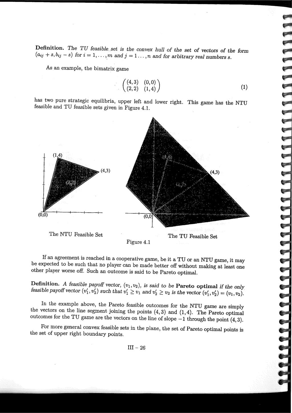
178 16