Boston, USA, August 5-11, 2012

Transcription

1 Session 4B: Measuring Economic Performance in China and India I Time: Tuesday, August 7, 2012 PM Paper Prepared for the 32nd General Conference of The International Association for Research in Income and Wealth Boston, USA, August 5-11, 2012 Growth, Regional Disparity and Convergence Clubs in India: A Sectoral Level Analysis and Decomposition Basudeb Chaudhuri Mainak Mazumdar Matthieu Teachout Velayoudom Marimoutou For additional information please contact: Name: Mainak Mazumdar Affiliation: Center de Sciences Humaines (CSH), India Address: mainakecon@gmail.com This paper is posted on the following website:

2 "Growth, Regional Disparity and Convergence Clubs in India: A Sectoral Level Analysis and Decomposition" Paper Prepared for the 32nd General Conference of The International Association for Research in Income and Wealth Boston, USA, August 5-11, 2012 By Basudeb Chaudhuri (Centre de Sciences Humaines, India) AND Mainak Mazumdar (Centre de Sciences Humaines, India) Corresponding author And Matthieu Teachout (École Polytechnique, France) And Velayoudom Marimoutou, GREQAM, Université de la Méditerranée For additional information please contact: Name: Mainak Mazumdar Affiliation: Center de Sciences Humaines (CSH) Address: mainakecon@gmail.com 1

3 Introduction: The Indian growth story has always fascinated scholars and policy maker. From a dismal growth rate, called the Hindu growth rate because of its stability, of 3.6 per cent in 1960 s, India has accomplished a growth rate of about 8 per cent in the post 2000 period, however, in spite of its achievement the fact that a large economy with considerable heterogeneity can have different regions growing with widely different growth trajectories gave rise to concerns about "unbalanced growth" and regional disparities. Studies focusing on the trends in the regional inequalities of the Indian economy have also concluded that there has been significant divergence in the growth rates of the Indian states and such divergence has been persistent over time see (Trivedi,2002); Bandyopadhyay,2002; Chaudhuri, Chevrou-Sévérac, Marimoutou,2006) Following the liberalisation of the Indian economy in and its fairly impressive growth over the past decade, led essentially by a certain number of Indian states, policy makers and researchers are concerned about the fact that some states are growing too slowly or not at all, and thus falling behind or failing to benefit from the opening up of the Indian economy and the dynamism of certain sectors and regions. In other words, apprehension about increased regional disparity has only heightened in recent years. To understand the disparity in the growth rates of the various regions of India, specialists of growth economics have also tried to verify in the context of large economies like India as to whether one of the predictions of growth theory, that less developed regions or countries will "catch up" with the more developed ones (through faster capital accumulation) is confirmed or not. This is often referred to as the "convergence" debate, and in the Indian context, empirical evidence points (Nagaraj, Varoudakis, Véganzonès, 1998) to the "divergence" in the growth path between Indian states, which is influenced by the initial conditions of social and economic infrastructure and human capital. In this paper we take 15 major Indian States, which represent around 90% of India.s population and also its considerable social heterogeneity. We do not include all the States in order to avoid problems related to the creation of new States over time. The inclusion of these States would not change substantively the results of our analysis and especially the important conclusions. By using a method called GUIDE, discussed further below, we generate endogenously 3 "clubs" of Indian States - "rich",(r), "transitional"(t), and"poor",(p) of the even though these terms are very relative in terms of international comparison. Our evidence is slightly more nuanced than the existing literature cited above and in the footnotes on this question in India; there is some evidence of convergence and similar movements or evolution within the clubs, there is divergence between the clubs, and there are a small number of 2

4 movements of some States between clubs. These movements, we shall argue, are significant in understanding the role of initial conditions and of thresholds or critical initial values of the relevant variables, such as income at an initial period. It enables understanding the case of multiple equilibria. The most striking element of our result is that over an important part of the period we are covering, there are three clubs and not two, and the presence of a transitional club with movements upwards and downwards might be a regular feature of large developing economies. In the context of our study we have also done the club convergence analysis at the sectoral levels; carrying out the club formation exercise at the sectoral productivity level enables us to reposition some fundamental questions of economic development, such as the role of agricultural growth (surplus) in fuelling subsequent growth in industry or services, and the importance of having an industrial sector to start with. Further analysis is necessary to answer these questions in a detailed way, but this preliminary convergence analysis will enable us to analyze the importance of sectoral growth for subsequent income growth. Finally, we have also examined the process of convergence across and between the 'clubs.' This has been achieved by decomposing the aggregate labor productivity of member states of the 'rich', 'transitory' and 'poor' clubs in its sectoral components and tracing its evolution over a period of time. The paper is therefore structured in the following manner. The next section provides some stylized fact about the growth experience of Indian States. In Section 3 we will briefly recall the concepts and tests of convergence and the present GUIDE methodology for our study. Results from GUIDE methodology has been presented in section 4. Section 5 explains and analyses the process of convergence for the clubs. This is followed by the concluding section. Section 1: Some Stylised facts about the Growth Experience of the Indian States The annual average growth rate of India in the first two decades was only 3.6 percent 2. It started accelerating at a rate of about 5 percent from 1980 onward, reaching 6 percent in the decades followed by the economic reforms of 1991(see table A4 column 17 in the appendix. By late 2000 the growth rate of GDP accelerated at about 7 percent (see table A4 column 17). In spite of such remarkable growth of the Indian economy, growth rates across the Indian states shows fair degree of variation. While it is true that the GDP of the states have grown at moderate rate in the last decade (i.e., in the early and late twenties) some states have done remarkable well and experienced rapid growth. To get a clear picture about 2 Given a population growth rate exceeding 2 percent in the first decades after independence, the per capita growth was below 2 per cent. 3

5 the extent of disparity in the growth rate across the states, we first consider the comparative growth trajectories of NSDP for 15 major states in India. In the sixties, Punjab and Haryana were the highest growing states with an average growth rate of around 5.5 percent (see column 6 and 12 in Table A4). The per-capita income of Punjab was also the highest (see column 12 in table A4). States like Maharastra, Gujarat, Kerala, Assam, Karnataka, and Rajasthan were growing either at 3 percent or more, which was close to all India average (see Table A4). The rest of the states like West Bengal, Tamilnadu, Madhya-Pradesh, Orisa, and Uttar-Pradesh were growing at merely 2 percent. Bihar was the poorest state with a growth rate of only 1.2 percent In terms of per capita-income, we do not find any discerning pattern in the growth of the states. Thus, while Punjab and Haryana were high growing states and also had the highest per-capita income, middle growing states like Maharashtra, Gujarat, also have high per-capita income level. It is interesting to note that in the decade of sixties low growing state like Tamilnadu had income level that is close to the income level of high growing states. Baring Bihar and UP that has the lowest per-capita income of.02 lakh per annum (lakh per annum?)and.03 the rest of the states had per-capita income of about.042 lakh. Contrary to the predictions of the convergence theory we therefore do not find that states that start up with low income were necessarily growing at a higher rate at least in the decade of sixties. When we rank the states in terms of the per capita income, the ordering of states changes ( see table 1A), while Punjab and Haryana still remains the states with highest growth, West Bengal slipped down and registered negative growth nature possibly due to high growth in its population. Kerela and Karnataka improved their position and grew at more than one percent. The rest of the states however, grew at less than one percent. Moving now to the decade of 1970, we find that Gujarat, Maharastra, and Andhra- Pradesh improved their growth rate from 3 percent to 4 percent. An interesting feature of this period is the marked improvement in the growth rates of the poor states like Bihar and Uttar- Pradesh from one percent to about three percent. We get similar picture even if we measure the growth rate of the per-capita SDP. From 1980 onwards the growth rate of the India started picking up; almost all the states improved their decadal growth rate in the period of 1980s. Haryana, Maharashtra, Andhra-Pradesh and Rajasthan were growing at a rate of about more than 5 percent followed by West Bengal, UP, Tamilnadu, Gujarat, MP, Karnataka and Punjab that were growing at more than 4 percent. States with low growth during this period are Assam, Kerela, Bihar and Orissa. If we evaluate the performance of the states by the growth rate of the per-capita SDP, we find more or less similar picture. However, the position of Assam and Kerela improves from low growing state to medium growing state and states with high population growth rate like Bihar and West Bengal slipped down. In general, there was a comparatively balanced regional growth during this period. The standard deviation of the 4

6 growth rate across the state reduces from 1.2 in the decade of 1960s to.96 in the decade of 1980s. In the period following liberalization i.e., in 1990s there was a dramatic churning up in the ranking of states. Medium growing states like West Bengal, Rajasthan, and Karnataka started picking up and were growing at more than 6 percent. The relatively industrial states of Gujarat and Maharastra were also growing at more than 6 percent, which was more than the all India average growth rate of the reform era. It is surprising to note that high growing states like Punjab and Harayana failed to keep up with the pace of all India average growth rate. States that have performed badly during these periods are Assam, UP, Bihar, Orissa and MP all of which had relatively low rates of growth to begin with. If we measure the per-capita growth rate, the Punjab and Harayana performance is the worst. Bihar improves its position due to a fall in its population growth rate and Rajasthan loses its rank due to the high growth in its population. 1990s was the period when the regional disparity in the growth rate was also the highest. The standard deviation in the growth rate was 1.39 in the period of 1990s. It is interesting to note that contrary to the popular perception, among the BIMARU states Rajasthan and Madhya-Pradesh performed well whereas UP and Bihar performed badly. Thus the commonly classified BIMARU states based on demographic behaviour, does not show any sign of homogeneity when evaluated in terms of economic performance. From 2000 to 2010, the growth rate of India has increased even further, almost all states have achieved higher growth rate during this period. Highly industrial states, of Gujarat and Maharastra improved their position substantially and grew at a rate of about 8 percent, close on the heels, were the states of Tamil-Nadu, West Bengal, Karnataka, Andhra Pradesh, and Kerela all of which grew at a rate of about 6 percent. It is note-worthy to mention that both Bihar and Orissa improved their position and grew at a rate of about 7 percent. States that have failed to pick up during this period are Assam, Punjab, and Madhya Pradesh. The standard of living measured in terms of per-capita income has improved substantially among the high and medium growing states. Maharastra, Gujarat, Punjab and Haryana have the highest per capita income followed by Tamilnadu, Karnataka, Kerela, West Bengal, Andhra- Pradesh and Rajasthan. In spite of having high growth rate Bihar still has the lowest percapita income followed by Orissa UP, Madhya-Pradesh and Assam. The dispersion in the standard of living measured roughly by standard deviation of income per-capita has however reduced across region over the decades it was 1.39 in 1990s, and it reduced to 1.15 in 2000s. 5

7 Section 1A: Sectoral Growth and Contribution of the States Sectoral growth rates, its share in the total GDP of the state and contribution in the GDP of India has been computed to understand the role of the principle sectors for the growth and transition of the GDP of the states and India. It is evident from the figures in table 2A that India has evolved from a underdeveloped economy with agriculture as the preponderant sectorto a new configuration with a service sector being the main contributor to GDP, thus bypassing the historical role of industries in the development processthus, in the decade of sixties the contribution of agriculture in the total GDP of India was 50 percent. This was followed by the contribution tertiary and the secondary sector. While the contribution of the primary sector in the total GDP has reduced to 20 percent in the recent decade and the tertiary sector contributed to more than 50 percent, the contribution of secondary sector has been quite modest. If we examine the figures of table 2A in the appendix we find the contribution of secondary sector in the total GDP has improved marginally from 19 percent to about 26 percent In other words, in the transition of the Indian economy from the primitive agricultural sector to modern service oriented state the contribution of the secondary sector has been sidestepped. If we however look at the growth rates of various sectors of India we notice that almost all the sectors started accelerating from 1980 onwards. The decade of eighties has been the turning point of the Indian economy and there has been a significant improvement over the period of stagnation that prevailed before (Ahluwalia, 1985). In the next two decades we noticed that both secondary and tertiary sector experienced significant growth with the growth of the tertiary sector outperforming the growth of the secondary sector. Consider now the primary sector, from a growth rate of 2.5 percent in the decade of 1970 India achieved a growth rate of 3.4 percent in the decades of eighties However, it started decelerating again and in the decade of late 2000 it was growing at a rate of only 2.7 percent. The poor performance of agriculture against the impressive growth of India would not have caused an increased disparity, had there been a decline in the proportion of labour dependent on agriculture. However, even now more than 50 percent of the workforce is dependent on agriculture. Let us now consider the sectoral growth and its composition in the total GDP of the states in India. Let us first consider the decades of sixties. The contribution of agriculture in the total NSDP pre-dominated for most of the states. For states like Andhra-Pradesh, Assam, Bihar, Haryana and Madhya Pradesh, the share of primary sector in the total GDP was more than 60 percent ( see table 2A in the appendix). However, the growth rate of primary sector was low and less than 1.5 percent with the exception of Assam and Haryana. The growth rate of the 6

8 primary sector in Assam was about 2.5 percent and Haryana was one of the states that had the highest growth rate in agricultural sector that was close to 5 percent. Agriculture contributed between 50 to 60 percent of the GDP for states like Punjab, Orissa, Rajasthan, Uttar Pradesh, Gujarat, Karnataka and Kerala and in Maharashtra, West Bengal and Tamilnadu the contribution of agriculture was less than 40 percent. Growth rate of the primary sector in Punjab was 5 percent, in spite of being a semi-arid zone, agriculture growth rate in Rajasthan was quite impressive and it was more than 3 percent. The growth rate of primary sector was 2.5 percent for Orissa, Kerela and Karnataka and close to 2 percent for West Bengal. Bihar and Tamilnadu had a very low growth in the primary sector and it was less than 2 percent. If we now consider the secondary sector we notice that the secondary sector contributed more than 20 percent in the total GDP of Gujarat, Rajasthan, Maharastra, Tamilnadu and West Bengal. For states like West Bengal and Tamilnadu the contribution of Secondary Sector was more than 25 percent. The contribution of the secondary sector in the total GDP for the rest of the states was barely close to 15 percent. The only exception was Bihar for which the secondary sector contributed even less than 5 percent. If we consider the growth rate of the secondary sector of India (that was 4.86 percent ) as the bench mark of our analysis we find, Haryana, Kerela, Madhya Pradesh, Punjab, Tamilnadu, Bihar and Karnataka experienced growth in the secondary sector that was much higher than the all India average. Close to the all India average was the growth rate of the secondary sector of Assam, Andhra Pradesh and Uttar-Pradesh. For the rest of the states like Gujarat, West Bengal and Orissa the growth rate of the secondary sector was below the all India average. When we take the case of tertiary sector we notice that for states like Kerela, Maharastra, Rajasthan, Tamilnadu, Uttar Pradesh, West Bengal contribution of Tertiary sector has been more than 30 percent. With the exception of Haryana for which the total share of the tertiary sector is less than 20 percent we notice that rest of states share of the tertiary sector was 25 percent. Haryana has the highest growth rate in the tertiary sector and that was close to 7.5 percent, this was followed by Punjab with a growth rate of about 6 percent. Other states that have high growth rate in the tertiary sector were Assam (5.34%), Kerela (5.53%), Madhya Pradesh (5.5%) and Maharastra (5.1%). The growth rate of the tertiary sector in Andhra Pradesh was (3.5%), Gujarat (3.6 %), Karnataka (4%), Orissa (3%), Rajasthan (3.2%) and Tamilnadu. For the rest of states like West Bengal, and Bihar the growth rate of the tertiary sector was quite low with Bengal registering a growth rate of only 2.7 percent and Bihar 2 percent. In the decades of seventies, we notice that the share of primary sector in the GDP of all states has reduced with a corresponding rise in the share of the secondary and tertiary sector. In its total contribution in the GDP, the share of the primary sector was still the highest followed by the share of the tertiary and secondary sector. The ranking of the states in terms 7

9 of the share of primary, secondary and tertiary sector in the total GDP has however not changed much. In terms of the growth rates, there have been some changes in the ranking of the states. Let us first consider the growth rate of the primary sector. It is interesting to note that high growing agricultural states like Punjab and Haryana experienced a fall in the growth of the primary sector in the decades of seventies. Other states for which there has been a fall in the growth of the primary sector are Karnataka, Kerala and Orissa. There has been a major improvement in the growth of the primary sector for states like Gujarat, Bihar, Maharastra, Uttar-Pradesh and West Bengal. Consider now the secondary sector, it is interesting to note that states like Andhra Pradesh, Uttar Pradesh, Bihar and Gujarat experienced a major growth in its secondary sector in the decades of seventies. Thus for example, the growth rate of secondary sector for Gujarat was 3.57 percent in the decades of sixties and it increased to 5.40 percent in the decade of seventies. In other words there was almost a rise of about 2 percent in the growth rate of the secondary sector in Gujarat. The growth rate of the secondary sector was also high for Uttar Pradesh from 4.09 percent to 6.43 percent. Other states that have experienced a rise in the growth of the secondary sector were Orissa, Rajasthan and Punjab. For the rest of the states there has been a fall in the growth of the secondary sector. States that have experienced a major fall in its growth rates of secondary are Madhya Pradesh and Kerela. Moving now to the case of the tertiary sector, we notice that majority of the states has experienced a rise in the growth rate of the tertiary sector from what it was experiencing in the decade of sixties. The rise in the growth of the tertiary sector for Bihar was also considerable.. From a mere 1.98 percent in the decade of sixties Bihar experienced a growth rate of about 5.6 percent in the decade of seventies. Other states that have experienced a massive rise in the growth rate of the tertiary sector are Gujarat, Andhra Pradesh, Karnataka, Madhya Pradesh, Rajasthan and West Bengal. The rest of the states have however, experienced a fall in the growth of the tertiary sector. Let us now consider the decade of eighties; the period the growth rate of GDP of India and majority of the states started picking up. If we consider the primary sector, states that have performed remarkably well in this period are West-Bengal, Tamilnadu, Madhya Pradesh and Kerela. West Bengal has the highest growth rate in the primary sector that is close to 4.5 percent. The fact that all these states has low growth rate in the primary sector in the last two decades implies a significant achievement in the growth of the primary sector for these states. Haryana, Punjab and Maharashtra maintained the high growth rate in the primary sector. Rest of the states maintained the same growth rate in the primary sector. If we now consider the secondary sector, eighties was the decade when majority of the states (except Assam and Bihar) experienced a significant growth in the secondary sector. Compared to their growth rate in the previous decade states that have done remarkably well during eighties are Andhra-Pradesh, Gujarat, Karnataka Rajasthan and Maharastra. Other 8

10 states that have also improved their growth rates are Madhya Pradesh, Kerela, Orissa and West Bengal. Rest of the states have maintained the growth of the previous decades or have marginally improved their position. To summarise we find that eighties was the decade when the growth rate of secondary sector of various states of India started gaining momentum. Let us now consider the tertiary sector, compared to the growth rate in the previous decade Andhra Pradesh, Gujarat, Karnataka, Maharastra, Rajasthan and Orissa have done remarkably well. States that have failed to maintain the growth in the tertiary sector are Assam, Bihar, Haryana and Punjab. Rest of the states has also experienced have however, experienced higher growth in the tertiary sector. On a whole we therefore find that in the decade of eighties most of the states has experienced a higher growth in the secondary and tertiary sector. We however, do not find any distinct pattern with the growth rates of the states in the eighties and the earlier decades. In other words, we do not find that states with lower growth rates in the various sectors were necessarily growing at a higher rate. Let us now consider the decade of nineties. Few states like Andhra-Pradesh, Gujarat, Maharastra and West Bengal experienced a high growth in the primary sector. However, the growth rate of the primary sector has plummeted for rest of the states. The contribution of agriculture in the total GDP of the states has also decreased in the decade of nineties. In the secondary sector, states that have achieved higher growth rate are Karnataka, Kerela, Madhya-Pradesh and West Bengal. States that have experienced lower growth rate in the secondary sector are Haryana, Punjab, Bihar, Andhra-Pradesh, Orissa, Uttar-Pradesh and Assam. The rest of the states have maintained the growth rate of the previous decade. On a whole we therefore find that many states have failed to maintain the pace of the growth in the secondary sector that they were experiencing in the previous decade. The tertiary sector has however, received a huge surge in its growth rate. Almost all the states barring (Uttar-Pradesh and Madhya-Pradesh) have experienced a important growth in the tertiary sector. States that have achieved almost 8-9 percent growth rate in the tertiary sector are Gujarat, Haryana, Karnataka, Maharastra and West Bengal. Other states have also experienced growth in the tertiary sector between 5 to 6 percent. In the decade of nineties, we therefore find that the tertiary sector in almost all the states have grown significantly. Finally, we consider the last decade of 2000; in contrast to the all India average we find that the growth in the primary sector started picking up for many states like Andhra- Pradesh, Bihar, Gujarat, Madhya-Pradesh and Orissa. At the same time we notice that there has been a sharp fall in the growth of the primary sector for states like Karnataka, Kerela, Tamilnadu and West Bengal. For the rest of the states the growth in the Primary sector was lingering at what it was experiencing in the previous decade. As expected the share of the primary sector has also reduced for almost all the states. High growing agricultural states like 9

11 Punjab and Haryana have failed to keep pace with the growth in its primary sector in the earlier decade and have slipped down. When we consider the growth in the secondary sector we find mixed outcome. Bihar and Gujarat experienced a phenomenal growth in the secondary sector growing at a rate of about 9.5 percent. Other states that have experienced a higher growth rate between 8.5 to 6 percent are Karnataka, Maharashtra, Haryana, Punjab, Orissa and Uttar-Pradesh. The rest of the states like West Bengal, Kerela, Tamilnadu and Rajasthan and Andhra-Pradesh have experienced a fall in the growth of its secondary sector compared to its growth in the earlier decade. Lastly, compared to its growth in the previous decade in the tertiary sector all states have experienced higher growth. However, there has been divergence in the growth of the tertiary sector among the states. States growing at the rate of about 11 to 9 percent are Haryana, Gujarat, Karnataka, Kerela, Maharashtra, Tamilnadu and West Bengal. States experiencing growth between 8.5 to 7 percent are Andhra-Pradesh, Assam, Bihar, Orissa and Rajasthan. The rest of the states i.e., Punjab and Madhya Pradesh were growing at a rate of about 6 percent. We therefore notice that the growth in the tertiary sector of the states is on rise even if they were growing at a high rate in the earlier decade. If we examine the trend in the sectoral share in the total GDP of the states we find that over the decades, the contribution of the primary sector in the total GDP has reduced phenomenally with the corresponding rise in the tertiary sector. However, only in a few states like Gujarat, Karnataka, Maharashtra and Tamilnadu, the share of the secondary sector in the total GDP of the states is higher compared to share of the primary sector. For states like Assam, Bihar, Orissa, Madhya-Pradesh, Punjab and Uttar-Pradesh, the share of the primary sector in the total GDP is close to percent. For the rest of the states like Andhra- Pradesh, West Bengal, Kerela, Rajasthan and Haryana, the primary and the secondary sector almost contributed equally in the total GDP of the states. Section 2: Concepts and Tests of convergence The analysis of growth from Solow onwards focused on understanding the relative role of factor accumulation (physical and human capital) and technological progress in understanding growth trends. Recall that the role of technological progress and also that of human capital were exogenous elements of the Solovian model. Subsequently, endogenous growth models starting from Romer (1986) incorporated endogenous technical change, the role of human capital and market structure in growth models, hence underlying the role of non-linearities in a growth process. As Durlauf and Quah (1999) summarize, models with nonconvexities, unlike the neoclassical Solow-Swan model, lead to long run dependence in the time series 10

12 properties of aggregate output. Nonconvex models can display poverty traps, where economies with low initial incomes or capital stocks converge to one steady state level of per capita output, while economies with high initial incomes or capital stocks converge to a di erent steady state level. As Durlauf, Temple and Johnson (2004) point out, there is disagreement on the empirical specification of growth non-linearities, or on means of distinguishing empirically neoclassical and endogenous growth models. The empirical method that we employ in this paper helps to highlight non-linearities and multiple equilibria in growth. The notion of convergence, which is a major subject of debate, is structured by the relationship between initial conditions and the long term output. The economic interest in convergence comes from the question of knowing upto what point the initial conditions lead to persistent divergences in the per capita output between countries or regions. There are three competing hypothesis in the convergence debate (see Galor, 1996 and Galor 2005) (i) the absolute convergence hypothesis: per capita income of countries converge to one another in the long run independently of the initial conditions ( In practice, one generally considers the stock of initial human and physical capital as initial conditions). (ii) the conditional convergence hypothesis : per capita income of countries that are identical in their structural characteristics (ex preferences, technologies, rates of population growth, government policies, political, institutional or geographical characteristics, etc) converge to one another in the long run independently of their initial conditions.(iii) the club convergence hypothesis (which analyses questions such as polarization, persistent poverty, clustering) - per capita incomes of countries that are identical in their structural characteristics converge to one another in the long run provided their initial conditions are similar as well. Initial conditions determine in an important way long run outcomes. Bernard et Durlauf (1996), Hall, Robertson et Wickens (1997) and Pesaran (2006) give definitions of convergence that that do not enable a distinction between the long term effects that are due to initial conditions and the long term effects that are due to structural heterogeneity. From the point of view of growth theory this is a serious limitation. In empirical research, it is important to be able to distinguish between the parameters of the initial conditions and the parameters of structural heterogeneity. The steady state effect of the initial conditions implies the existence of convergence in clubs while the steady state effects of structural characteristics do not. The expression of these ideas in the regression equations of growth models have led to a certain number of statistical definitions of convergence such as beta convergence and sigma convergence. There is a fair amount of evidence of conditional beta convergence (ie beta convergence in the presence of control variables such as population and growth-rates). However, there is a problem in using beta convergence when one wants to test between the Solow model and a model with multiple stable steady states - these models clearly violate the economic idea of convergence since 11

13 long run behaviour in the model depends on initial capital stock (Durlauf, Kourtellos, Tan 2005). Bernard and Durlauf (1996) show for example that it is possible for data generated by economies that are described by Azariadis Drazen model, with a discontinuity in the aggregate production function, to exhibit beta convergence even when multiple steady states are present. The reason is that even if economies are converging to distinct steady states the economies converging to a low steady states may be growing faster than those converging to a higher one. Beta convergence does not provide insights as to whether cross sections of countries that exhibit differences are transient or permanent. In order to overcome the problems raised by beta convergence, another range of models study the dispersion of income differences over time - there is sigma convergence if cross section standard deviation of income is falling over time. The CART method of Breiman et al (1984) enables the endogenous determination of clubs by using regression trees. Subsequently one can study the evolution of the standard deviations in these clubs. Loh (2002) improves the CART method using Generalized Regression trees to develop a method called GUIDE. We use this method, outlined in some more detail in the appendix, to detect clusters of economies, depending on their initial conditions. In this paper the formation of the clubs has been accomplished by using two different methods: the first one is by using the year-by-year method and the second the relative-toothers method Section 3: Finding clubs: the year-by-year method In the year by year method, we consider each year as a single cross section. The dependent variable in the model is the real income of the states and the independent variable that is used to split the cross sectional data is the past values of the income of the states. Thus, for example if y i, t is the real income of the ith state in the t th period, then the splitting variable considered in the model are yi,t-1, yi,t-2 and so on. More precisely, for forming a club in say 1980 the algorithm chooses whether income in 1979, 1978.or 1965 is the BEST variable to split the sample (15 states) and minimize the variance. The table below summarizes the result from our analysis. From 1970 to 2007, we obtained mainly two clubs, Rich and Poor. Three clubs have been obtained only for a very few years. The clubs are available in the table below. When we have only two clubs, they are called the Rich(R) club and the Poor (P) club and when we have three clubs, they are named the Rich (R), the Poor (P) and the Transitory(T). The distribution in clubs along the years is quite scattered. Though, one can notice that Gujarat, Haryana, Maharashtra and Punjab have consistently belonged to the rich club (in orange in the table). Conversely, Uttar Pradesh, Orissa and Bihar have consistently belonged 12

14 to the poor club (in blue in the table). Rajasthan, Madhya Pradesh and Assam except for a very few years have been in the the poor club (in light blue in the table). In between, some states have had a more volatile path (in green). For the period 1970 to 1983, the composition of the clubs has not changed at all along the years. One very important remark is that for every year, the variable used for splitting the sample is always the real income in 1966 and not the income of the next years. This shows how important the income at the beginning of the period has been for explaining the states income distribution for the preceding years. Between 1983 and 1990, Andhra Pradesh, Karnataka, Kerala leave the poor club and form a transitory club which enters the rich club at the end of the period. This progress is halted between 1991 and 1993 and all of them fall back in the poor club in less than 3 years. After 1994, Andhra Pradesh, Karnataka and West Bengal start a 6 years process to catch up with the rich club and from 2000 to 2007, the composition of the clubs is constant except for West Bengal that falls back in the poor club in

15 From 1984 to 2007, the splitting variable is SDP of the previous year except for 1993 to 2000, where the variable is SDP in 1966! This striking result shows that even after 30 years, the income of the beginning of the period was still the key for explaining the distribution of the income of the recent year. It also exhibits that, for 30 years, very few movements between states have occurred. Section 3.1: Looking for polarization: the relative-to-others method The regression tree analysis carried out in the previous paragraph minimizes the cross state variance in each club year by year. An alternative way of examining the club convergence and inequality among the states is to use the relative-to-other methods. In this method, for each year, we divide the income of one state by the average of all others'. This methodology also enables us to study polarization. If one state falls into a poorer club it means that its income relative to others has decreased. It is similar to considering that India has a natural growth rate and to see which states benefit from it. The variable used for splitting in the lagged income divided by the mean of income that year, so that the number of variables is the same for all the years. The dependent variable is therefore: yi, t yˆ i, t = N and the splitting variable: y ˆi, t. We y first consider the NSDP per capita of the state as the principle variable of our study; we also allow the regression tree to have a maximum of 3 variables. i= 1 N i, t Section 3.1.1: Regression Tree for NSDP Per Capita We obtain the following structure for the tree by running the regression analysis We have 200 observations for club 1, for club 2 we have 244 observations and 291 observations for club 3. The mean income for the club 3 which is also the rich club is 1.35 and the mean income for the club 2 the transitory club is.92 and poor club

16 One can first notice, that more than two thirds of the sample are under the value yt-1=1, which means that more states' income were below the mean income along the years that emphasized the growing inequality among the states. We next look at the distribution of the states in each club along the years. The results are given in the table 1 below. Table 1: Distribution of States using NSDP per Capita as the Dependent Variable Year AP ASS BIH GJT HYN KNK KRL MP MHR ORS PJB RJT TN UP WB

17 We consider four sub-periods: , , , , that is, around four decades that correspond to distinct periods in India's growth. We obtain three clubs of states for all the period. For the first period, , we have only three states in the poor club, Bihar, Madhya-Pradesh and Uttar-Pradesh and 6 states, Haryana, Gujarat, Maharashtra, Kerala, Punjab and Tamilnadu in the rich club. The rest of the states like Andhra-Pradesh, Assam, Orissa, Karnataka, Rajasthan and West Bengal were in the transitory club. There was not much co- movement of states among the three clubs except for the fact that West Bengal dropped from the rich club to the transitory and Madhya-Pradesh from transitory to poor. In the period , Kerala dropped from the rich to poor club and Assam, Rajasthan and Orissa from transitory to poor state. Between 1981 to 1990, Assam and UP recovered from poor to Transitory state, for the rest of the state there was no movement from one club to another. After 1991, i.e., the liberalisation of the Indian economy, there re-grouping of the states has taken place. Karnataka and Kerala moved into the rich club, and Assam and Rajasthan dropped in the poor club. Section 3.2: Regression Tree for the Productivity of the States: We have also undertaken the regression tree analysis using the aggregate productivity of the states as the variable of our study. Measuring productivity is a better way to evaluate the performance because it also takes into consideration the inputs used in the production process. Thus, instead of using the income per capita, the dependent variable is now the productivity of the states. However, due to the lack of data on capital and other inputs in the production of output we measure the partial sectoral labour productivity where Labour productivity of the ith sector is measured as the output produced by the ith sector divided by the labor employed in the sector. We get the following tree using the productivity of the states. Using the productivity of the states as the variable for our analysis we find that there are again three clubs of states, rich, poor and transitory. Using the productivity of the states as the variable for our analysis we find that there are again three clubs of states, rich, poor and transitory. For the aggregate productivity, we have for Club 1: 200 observations, Club 2:

18 observations, Club 3: 303 observations. An important observation that we find from the regression tree analysis for the aggregate productivity and NSDP per capita is that there is more heterogeneity between the poor and other groups of clubs than between the rich and the transitory club in term of mean income of the member states. Table 2: Regression Tree using Productivity as the Variable for Analysis Year AP ASS BIH GJT HYN KNK KRL MP MHR ORS PJB RJT TN UP WB The ranking of the states has not changed much even if we consider the productivity of the states. We however found that the distributions of the states are stable and a clear pattern of 17

19 polarization emerges. States that have significantly improved their position are Tamilnadu and Karnataka. Tamilnadu has improved its position from the transitory state to rich state long back in the decade of seventies. Since then it has remained in the rich club. The movement of Karnataka from transitory to rich club has however, taken place quite recently only after the economy was liberalized. Andhra-Pradesh is another state that has improved its position from poor to transitory state in the decade of seventies. Andhra Pradesh, in spite of the developments in information technology and services in Hyderabad, does not show a more substantive acceleration to catch up with the rich group which was however, not the case for Karnataka. States that have deteriorated their relative position are Orissa and West Bengal of which Orissa has dropped from the transitory to poor state and West Bengal from rich state to transitory state. At this point, we can speculate that we observed a phenomenon of polarization with a three club situation. The situation could correspond to a multiple regime situation with two equilibria as in Azariadis-Drazen (see Galor 1996). Note that Bihar, U.P., Orissa, Assam and Madhya-Pradesh form the poorest group. In this group, it can be remarked that Bihar and Madhya-Pradesh (minerals) and Assam (timber, oil, tea) are resource rich yet undeveloped states like many countries in Africa. We see in the Indian context the use of regression tree method help us to identify clubs of States that apparently obey a common model. This would point to the fact that initial conditions play an important role in their trajectories, and also that the growth rate behaviour corresponds to multiple steady states. In this paper, we are not dealing with the determinants of growth - we are just tracing the evolution of per capita income of the States to see how they "club" together according to common characteristics, and notably to see the role of initial values of per capita income. A quick look at the descriptive statistics of each club therefore gives more insights about the details of the clubs. 18

20 The table below furnishes the mean value of the principle variables for each group for different decades. Table 3: Description of the principle variables (mean value) Growth NSDP Rich NSDP Per Capita Rich(in INR) Growth Per capita(total Productivity Effect) Rich Growth Per capita Transitory NSDP Per Capita Transitory (in INR) Growth Per capita(total productivity Effect) Transitory Growth Per capita Poor NSDP Per Capita (Poor)(in INR) Growth Per capita(total Productivity Effect) Poor Average Max Min Average Max Min Average Max Min Average Max Min Average Max Min Certain interesting point comes out from the figures in table 3. First, differences in the NSDP per-capita between the rich and the transitory club in the earlier decade of 1960s were not much. Simple calculation reveals that the per-capita income of the rich club was higher than the transitory club by only 13 percent. On the other hand the differences in the per-capita income between the rich and poor club was 60 percent and 41 percent between transitory and poor club. Over the years the per-capita income between the rich and poor club has magnified manifold and in recent decade the mean income of the rich club is 151 percent higher than the poor club. Between the rich and transitory club the gap in the per-capita income has also increased. The gap was highest in the decade of eighties and per-capita income of the rich club was higher than the club transitory club by about 66 percent. However, the decades following the liberalization of the economy the gap in the income between the rich and the transitory has reduced and in the per-capita income of the rich club is higher than the transitory club by 40 percent. Between the decade of eighties and nineties, the rich club has experienced growth in the per-capita income by 28 percent and the transitory club by more than 49 percent and poor club by 39 percent. In the last two decade the per-capita income of the rich club has increased by 53 percent and the transitory club by 54 percent. In contrast, the increase in the per-capita income of the poor club was 37 percent. Secondly; if we compare the growth rates in the NSDP we find that even the rich club had much higher growth rate than the transitory and the poor club in the decade of sixties and seventies. In the next decade the growth rate of the transitory club picked up and it was the highest among all the three clubs for two decade. In the recent decade, the growth rate of the NSDP of the rich club has 19

21 again picked up and was the highest. The ranking of the clubs however changes when we evaluate them with the productivity growth. In the earlier decade of 1960s the productivity growth of the rich club was negative and lowest among all clubs. In contrast, the productivity growth of the transitory and poor club was positive with the transitory club having the highest productivity growth. In the next two decade the productivity growth of the clubs was negative although the intensity of the fall in the productivity growth for the rich club was the lowest. Productivity growth recovered and turned positive for all the clubs only after the opening up of the economy in the nineties. It started accelerating and the rich club overtook the transitory and the poor club in the recent decade. It was 5.76 percent for the rich club in the recent decade followed by 5.06 percent for the transitory and 4.09 percent for poor club. To summarize we find that it is the rich and the transitory that has benefitted most from the opening up of the economy. Section 3.3: Sigma Convergence in the Club In order to study convergence, we have to look at the evolution of the standard deviation in time. We have measured the standard deviation for NSDP per capita and the productivity for the three clubs. Figure 1: Standard Deviation of NSDP per capita Figure 1: Standard Deviation of aggregate productivity 20

22 It is evident from the figures, that the standard deviation of the productivity of the states is stable for the three clubs of states than the standard deviation of the NSDP per capita which is more volatile. The standard deviation of productivity declines faster steadily for the rich club till 1975; after 1975 it was more or less stable and declines marginally. Figures for the standard deviation of the income for the rich club indicate that it declines with swings. It increased in the decade of 1980 and then declined with a further increase in the mid of last decade before it plunges down again. The standard deviation for the NSDP and the productivity for the transitory club are more volatile than the poor club partly because of the entry and exit of new members in the club. An interesting observation that is evident from the figures is that the standard deviation of the poor and transitory club increased between 1985 and 1995, when the economy was recovering from the state of low growth rate and was opening up to new market opportunities. From 1995 onwards there is clear evidence of fall in the standard deviation of the rich and poor club which continued till the end of the last decade. Section 3.4: Sectoral Convergence The club-convergence analysis has also been conducted at the sectoral levels treating the productivity and the NSDP from the three principle sectors viz., primary, secondary and tertiary as the principle variable of our study. We first consider the tertiary sector that has principally driven the growth of the NSDP of the Indian Economy. Table 4 furnishes the information from the analysis. 21

23 Table 4: Clubs with NSDP from Services Year AP ASS BIH GJT HYN KNK KRL MP MHR ORS PJB RJT TN UP WB It is interesting to note that the regression tree has generated two clubs for NSDP from the service sector rich and poor indicating clear pattern of bi-polarization. From the figures in the table it is evident that Maharashtra, Gujarat, Kerala, Punjab and Tamilnadu have remained consistently in the rich club and Assam, Bihar, Uttar-Pradesh, Orissa, Madhya-Pradesh and Rajasthan has always remained in the poor club. West-Bengal is the only state that has fallen back from being the rich state to poor state and has recovered its position in the rich club in the mid of nineties. Haryana and Andhra-Pradesh has improved their position from poor to rich club in the latter half of the mid eighties and Karnataka has moved in the rich club only recently in the mid of nineties. Such clear pattern of bi-polarisation is however, not evident 22

24 when we rank the states on the basis of their productivity in the service sector. The table 5 below summarizes the distribution of the productivity in services of the Indian states. Table 5: Club with Productivity of Services Year AP ASS BIH GJT HYN KNK KRL MP MHR ORS PJB RJT TN UP WB Once again we find that the regression tree has generated three clubs, rich, poor and transitory. Maharastra is the only state that has remained in the rich club for the service right from the decade of It is not surprised given the high concentration of the service related activities in the financial capital of India Mumbai. Gujarat is another state that was in the rich club in the decade. What turns out to be interesting is that poor state like Orissa and Rajasthan were in the rich club when we consider the productivity of the service sector and Karnataka 23

25 which is now the IT hub of India was in the poor club. States that were in the transitory club were West-Bengal, Punjab, Madhya-Pradesh, Tamilnadu and Kerala. The rest of the states were in the poor club. There was also some movement of the states from one club to another in the decade of sixties. Thus, West Bengal and Punjab improved their position from transitory to rich club and Madhya-Pradesh deteriorated its position from rich to poor club and Rajasthan from rich club to transitory club. Certain movements of the states between the clubs were also noticed in the next decade. Gujarat deteriorated its position from rich to transitory club, Orissa from rich to transitory to poor club and Rajasthan from transitory to poor club. UP improved its position from poor to transitory club and West Bengal from transitory to rich club. By the end of the decade Gujarat also improved its position from transitory to rich state. The distribution of the states has also changed in the decade of eighties. The states that have improved their position are Haryana, Rajasthan and Andhra- Pradesh from poor to transitory state and states that have moved down are West Bengal and UP from rich to transitory state and Kerala from transitory to poor state. After the opening up of the economy in the decade of nineties the tertiary or service sector received a big impetus for growth. It was Karnataka that has benefitted most from the IT growth. In less than a decade it has improved its position from poor to transitory to rich club all because of its IT hub in Bangalore. The other state that had improved its position was Tamilnadu from transitory to rich club and Kerala from poor to transitory club. States that have fallen back in the decade of liberalization are West Bengal and Uttar-Pradesh from transitory to poor state. In the last decade it was Haryana that has improved its position from transitory to rich state and West Bengal from poor to transitory state. Two states that have failed to keep its position are Punjab and Rajasthan that has moved down to poor club in the service sector. Let us now consider the club formation for the secondary sector. The table 6 furnishes the information about club formation of NSDP from the secondary sector. Certain interesting insights that we get from the analysis are as follows: First, Maharashtra, Gujarat and Tamilnadu has always remained in the rich club and Kerala in the transitory club right from the decade of early sixties to the present time. On the other hand, Bihar and UP has always remained in the poor club. States that have improved their position are Haryana, Punjab, Karnataka from the transitory club to rich club in the decade of sixties, eighties and nineties respectively and Andhra-Pradesh and Madhya Pradesh from poor to transitory club in the decade of eighties and nineties. 24

26 Table 6: Clubs with NSDP of the Secondary Sector Year AP ASS BIH GJT HYN KNK KRL MP MHR ORS PJB RJT TN UP WB States that have deteriorated their position are West Bengal from rich to transitory club and Assam and Orissa from transitory club to poor club. 25

27 Table 7: Clubs for Productivity in the Secondary Sector Year AP ASS BIH GJT HYN KNK KRL MP MHR ORS PJB RJT TN UP WB The distribution of the states is however, not so stable when we run the regression tree with the productivity in the secondary sector and there has been instances of movement of states from one club to another. While Gujarat and Maharashtra still remained in the rich club, consistently from the decade of sixties, Tamilandu lost its position from rich to transitory club in the decade of nineties. Another state that has consistently remained in the rich club was Haryana. States that have improved their position are Punjab and Karnataka from transitory club. Punjab improved its position as early as the decade of seventies and Karnataka only 26

28 after the liberalization of the economy. The case of Assam turned out to be interesting; it was in the transitory club from 1961 to 1963, from 1964 to 1998 Assam was in the rich club. Its position fell from rich club to transitory in 1999 and it further tumbled down in the poor club from 2007 onward. Given the instable political climate and its association in the poor group for long it is difficult to give a plausible explanation for high productivity in the secondary sector. The position of Kerala, Madhya-Pradesh and Uttar-Pradesh was quite volatile. From poor club Kerala improved its position to the transitory club in the decade of late sixties and remained there till 1993; from 1993 to 1997 it fell back to poor club, recovered its position to the transitory club which was however not lasting and it fell back to the poor club again in Uttar-Pradesh was in the poor club in the earlier decade of sixties and seventies; it recovered its position from poor to the transitory club in mid seventies and slipped down to the poor club again from 1994 onward. Madhya-Pradesh was in the poor club in the early decade of sixties; it then improved its position and moved to the transitory club in late sixties, it fell back to the poor club in 1982, recovered and stayed in transitory club from 1990 onward. West Bengal was in the rich club in up to the decades of sixties; it slipped down to the transitory club in the decade of early seventies and by late seventies in fell back in the poor club and never recovered from there. Club formation with NSDP and Productivity from the Primary Sector 27

29 Table 7: Clubs with NSDP from primary sector Year AP ASS BIH GJT HYN KNK KRL MP MHR ORS PJB RJT TN UP WB

30 Table 8: Clubs with Productivity from the primary sector Year AP ASS BIH GJT HYN KNK KRL MP MHR ORS PJB RJT TN UP WB Consider now the NSDP from the primary sector, historically Punjab and Haryana were agriculturally rich state and they have always remained in the rich club for four decade. Gujarat undertook various institutional reforms to improve the agricultural produce right from historical times and it also remained in the rich club all along. States that have remained consistently in the poor club are again Bihar and Uttar-Pradesh and Karnataka and Rajasthan are the state that has remained in the transitory club for four decades; for the rest of the states there have been movements across the groups. Consider, West-Bengal which has successfully 29

31 initiated land-reform in the decade of seventies. However, in spite of the reform state has persistently remained in the poor club for three decades. It is only in the late eighties; West Bengal improved its position and moved to transitory club. States that have lost their position are Kerela and Tamilnadu, Kerala moved from being a member of the rich club to transitory club and in the end poor club. We get similar pattern for Tamilnadu and Assam. We get a clearer pattern by running the regression tree with the productivity of the primary sector. Haryana, Gujarat and Punjab still retained their position in the rich club, Bihar and Uttar-Pradesh in the poor club and Tamilnadu and Karnataka in the transitory club. States that have improved their position are West Bengal from transitory to rich club only after the mid nineties and Andhra-Pradesh from transitory to rich club only in the recent years. States that have failed to maintain their position are Orissa. Orissa was in the transitory club till mid eighties, it then dropped in the poor club and recovered its position only the last two years 2008 and Assam was in the transitory state for almost four decades and only lost its position in the recent decade of early twenties. Section 4: Structural Change and the Mechanism of Convergence across the Clubs A central insight of economics is that development entails structural change. Countries or regions that can pull its labor and resources from agricultural or other low productive activities to modern economic activities are able to expand their income and increase their over productivity. Poor regions or countries are characterised by large productivity gaps. It was Arthur Lewis who first conceptualised the duality in the economic structure of less-developing countries. Such gap in productivity differentials between the various sectors of the economy are indicative of allocative inefficiencies that reduce overall labor productivity. If economy can pull out its resources from less productive regions to productive sectors then it can grow even if there is no productivity growth within sectors. Redistribution of resources from the low productive sector to high productive sector without any corresponding growth in the productivity within sectors is known as structural effect change?. In other words, productivity growth can take place either due to structural effect or due to intra-sectoral change i.e., productivity growth within sectors or it can also occur due to the interaction between the two forces. In the context of our analysis we want to examine the extent of dualism prevalent in the rich, transitory or poor club and want to identify whether and to what extent the structural and the intra-sectoral change has contributed to the overall productivity growth of the economy of the states. This section is primarily devoted to such analysis. 30

32 Section4.1: A Sectoral Decomposition Analysis of Productivity growth of the Indian States and its convergence Growth in the labour productivity in an economy can be accomplished primarily in two ways. First, keeping the employment level of labour constant productivity within economic sectors can grow through technological and efficiency improvement in production. Secondly, labour can move across sectors from low productive sector to high productive sectors, increasing the overall productivity in the economy. The first effect is known as the intra-sectoral effect and the second the structural effect. The structural effect can be further decomposed into two effects: the static sectoral effect that takes places through the reallocation of labour to more productive sector or to sectors with higher labour productivity growth rates (dynamic sectoral effect). This can be expressed using the following decomposition Y Y0 ( ) L1 L Economy Wide Productivity Growth 1 n y n n j1 y j0 y j0 y j1 y j0 = θ j0( ) + ( θ jt θ j0) + ( θ jt θ j0)(...(1) j= 1 l j1 l j0 j= 1 l j0 j= 1 l j1 l j Intra-sectoral Effect Static sectoral Effect Dynamic Sectoral Effect ) Structural Effect Y y 1 j is the economy wide labor productivity and is the sectoral labor productivity in the L l 11 final period. θ jt is the share of employment in sector j at the final period. The first term in the decomposition is the weighted sum of the productivity growth within individual sectors where the weights are the employment share of each sector at the beginning of the period. We call this the Intra-sectoral Effect. The second term captures the productivity growth due to the reallocation of labour across different sectors which we call this the structural effect. It is essentially the sum of two components viz., (i) the inner product of productivity levels (at the beginning of the time period) with the change in employment shares across sectors and (ii) inner product of the change in the productivity and the change in the employment shares of the sectors. When employment share is positively correlated with the productivity change this term will be positive, and structural change will increase economy wide productivity growth. In this paper we have decomposed the labour productivity growth of the Indian states to understand the mechanism of productivity growth of the states. In the next step we have regressed the decomposed component from the first step on the logarithm of initial output per worker to obtain the β-decomposition across the rich, poor and transitory club of states to understand to what extent the various component of the productivity growth explains the j 31

33 convergence among the states in the group. In other words by undertaking the regression analysis we get the following β-decomposition. n β = βproductivi ty Growth in Sector j + βintra -sectoral Effect + βstatic-sectoral Effect + β j= 1 Dynamic Effect (2) In the above equation β is aggregate convergence coefficient that is obtained from regressing aggregate productivity growth on obtained by estimating the other component on ln yo and the subscripted β s are the co-efficient ln yo. Section 4.2: Intra-Sectoral and Structural Change Across States: Before we present our results from regression analysis let us explain the pattern of productivity change for rich, poor and transitory club. Table 9: Productivity growth and its component for Clubs Rich Productivityprimary) Productivitysecondary) Productivity- Tertiary) Intra- Sectoral Effect Growth Per capita (Static- Sectoral Effect) (Dynamic Effect) Structural Effect Total productivity Effect Transitory Poor Consider first the states from the rich club. If we examine the average aggregate productive growth of the rich states, we find that its growth in the total productivity was negative in the earlier decade of 1960s. In other words, states that started with high level of initial income 32

34 had negative aggregate productivity growth in the decade of If we compare the total productivity growth of the rich club with the transitory and poor club we find that states from the transitory and poor club had higher aggregate productivity growth than the rich club. In other words, states with lower level of initial income were growing at a higher rate. In the next two decade, the aggregate productivity growth was still negative for states from the rich, transitory and poor club, though the intensity was less for states from rich club. In the last two decade, productivity in the rich club improved and it experienced positive growth. Thus after liberalisation in the decade of nineties the productivity growth of the rich club was 3.3 percent and in the late twenties it was 5.8 percent. The transitory club also experienced positive productivity growth and in the nineties it has a growth rate of about 4 percent that was higher than the productivity growth of the rich club. Even the states from the poor club had flared well and experienced a productivity growth of around 2 percent in nineties which increased to about 4 percent in the decade of twenties. To summarise we notice that states that started with initially higher level of income are still growing at a higher rate in the current decade. Let us now compare the productivity growth of primary, secondary and tertiary sector across the rich, transitory and poor club. Consider first the productivity growth of the primary sector. We again find that in the decade of sixties the productivity growth of the rich club was negative and lesser than the transitory and poor club. Consequently, over the years it has improved its productivity in the primary sector but on an average the productivity growth in the primary sector was always lesser than the transitory and poor club. If we now consider the secondary sector we find the productivity growth of the secondary sector was higher in the poor club in the decade of 1960; in the next three decade it plummeted down and productivity growth was negative. In contrast the productivity growth was positive and higher in the decade of eighties, nineties and even in the recent decade for the rich and transitory club. However, in the decade of eighties and nineties the productivity growth in the secondary sector was higher in the transitory club than the rich club. In other word, secondary sector played a major role for productivity growth in the rich and transitory club. Lastly, if we consider the tertiary sector we notice that productivity growth of the tertiary sector was much higher in the rich and transitory club than the poor club. In fact, figures in the table suggest that productivity growth in the tertiary sector was even higher in the transitory club than the rich club till the decade of nineties. We now examine the channel of productivity growth for the three clubs of states. We note that structural change has played a major contribution in the productivity growth for all the three groups of states in the decade of However, its contribution was less for rich clubs and highest for the transitory clubs in the decade of 1960s. Figures in the table indicate that in 1960 the structural change contributed about 2.3 percent of the economy wide productivity growth of the transitory club. In labour has moved from the low productive 33

35 sector to the high productive sector in the decade of 1960 for all the three club of states. On the contrary the intra-sectoral effect was negative in 1960 for all the three group of states the magnitude of which was which was highest for the rich states. It remained negative for the next two decade for the three groups of states. The intensity of the fall in the intra-sectoral effect was highest in the decades of seventies and magnitude of which reduced in the next decade of eighties phenomenally. Thus from a sizeable negative contribution of about 5 percent in 1970s, the negative contribution of intra-sectoral effect was only.5 percent for the rich club, 1 percent and 1.4 percent for the transitory and poor club. The contribution of the structure change to bring about productivity growth for the rich, poor and transitory club has also reduced in the next two decade and figures in the table suggest that structural change has made a very little contribution to the overall growth in labour productivity for all the three group of states in the decade of seventies and eighties. After liberalisation of the economy, labour productivity growth was mainly propelled by intra-sectoral effect. In other words from a negative growth in the last three decades of sixties, seventies and eighties, in the decades of nineties and twenties all group of states registered a positive growth in their intra-sectoral effect. What determines then the economy-wide performance in these states is, by and large, how productivity fares in each individual sector. Figures in the table suggest that intra-sectoral effect contributed to about 2.7 percent of the economy wide labour productivity for the rich club 3.5 percent for the transitory club and only 1.4 percent for the poor club. In the last decade, the contribution of the intra-sectoral effect was even higher and we notice that for the rich club it was as high as 5 percent for the transitory it was 4.4 percent and for poor club is 3.2 percent. In contrast the contribution of structural change was marginal and less than even one percent after liberalisation, indicating that there was lesser movement of labour from the low productive to the high productive sector and that the extent of dualism in the economy was also high. However, the contribution of the structural change was about.61 for the rich club followed by the transitory (.50) and poor club (.49). The ranking of the states however changed in the last decade and it is structural change of the poor club that contributed most almost one percent to the overall growth of their economy, followed by the transitory and rich club of states. β Convergence and its Decomposition We next conduct the regression analysis to check for aggregate β convergence - for the whole sample as well as for the rich, poor and transitory club. As stated in the previous section, the aggregate β convergence coefficient is obtained from regressing the aggregate productivity growth on lny o. While estimating the beta coefficient we typically follow the 34

36 Mankiw, Romer and Weil (1992) framework and utilize the panel structure of our data. The equation that we estimate is then as follows ln( yit ) ln( yi, t 1) = β ln( yi, t 1) + µ i + ε it (3) y it is the productivity of the state i at time t. µ i is the state specific fixed effect, which pick up the influence of any omitted variable that does not vary with time in a panel. ε it is the transitory error term that varies across countries and time periods, and has mean equal to zero. and, the coefficient β identifies the convergence effect. The table 10 below summarises the result from the regression analysis for the whole sample i.e., all states taken together Table 10: Convergence for the whole sample Independent Variable Ln aggregate Productivity Dependent Variable : Productivity Growth Coefficient z P> z Model Random/Fixed R-square Overall Random Dependent Variable Ln (Aggregate Productivity) Productivity Primary Random Productivity Secondary Random Productivity Tertiary Random Intra-Sectoral Effect Random Static Sectoral Effect Fixed Dynamic Effect Random Table 10 reports the results from the regression analysis. It is evident from the available statistics of the table state specific intrinsic effects are significant. The estimated Hausman statistics suggest that the appropriate model for estimation is the random effect model. The 35

37 coefficient from the estimation suggest that for the whole sample the aggregate β convergence is estimated to be.03 percent, which is statistically significant at 5 percent level. The productivity growth in the tertiary sector accounted for 1.47 percent point that is more than 100 percent of the aggregate β convergence. The effect is statistically significant at one percent level. Productivity growth in the primary and secondary sector has however led to divergence among the states. The pure sectoral productivity growth which is captured by the Intra-Sectoral Effect also turns out to be negative but statistically insignificant because the convergent effect from the productivity growth in the tertiary sector has been masked by the divergent effect from the primary and secondary sector. It is interesting to note that the contribution to convergence from the employment shift is negative and it is statistically significant at one percent level with positive coefficient. In other words, employment flow has led to aggregate divergence. Such effect has happened because there has been a reversal of employment from the tertiary sector to the primary and secondary sector. The dynamic effect which captures the productivity growth due to the interaction from the employment flow to the more productivity sector and productive growth of the sectors is statistically highly significant and explains the convergence across states by.42 percent point. The regression analysis has also been done separately for the rich, poor and transitory club to examine the process of convergence for the three groups of states. Consider first the rich club; Table 11 captures the result from the regression analysis for the rich club Table11: Convergence for rich club Independent Variable Ln aggregate Productivity Dependent Variable : Productivity Growth Coefficient z P> z Model Random/Fixed R-square Overall Random Dependent Variable Ln (Aggregate Productivity) 36

38 Productivity Primary Random Productivity Secondary Random Productivity Tertiary Random Intra-Sectoral Effect Random Static Sectoral Effect Random Dynamic Effect Random Table 11 reports the results from the analysis. It is again evident from the table that state specific intrinsic effects are significant. The estimated Hausman statistics again suggest that the appropriate model for estimation is the random effect model for the rich club. The coefficient from the estimation suggest that for the whole sample the aggregate β convergence is estimated to be.02 percent, which is however not statistically significant. The estimated R-Square suggests that the overall predictability of the model has not improved for the regression equation for the rich club. However for the second regression model the R-Square value suggest that there has been significant improvement in the predictability of the model. Also all the co-efficient are statistically significant at one percent level. The estimated co-efficient of the model suggest that it is only the productivity growth in the tertiary sector that accounted for the aggregate β convergence. However, it accounts for.03 percent of the total convergence. We again find that the productivity growth in the primary and secondary sector has however led to divergence even among the member states in the rich club. The pure sectoral productivity growth which is captured by the Intra-Sectoral Effect turned out to be positive and statistically significant. In other words, Intra-Sectoral Effect is leading to divergence among the member states. Again we find that contribution to convergence from the employment shift is negative and it is statistically significant at one percent level. In other words, employment flow has also led to aggregate divergence. The dynamic effect which captures the productivity growth due to the interaction from the employment flow to the more productivity sector and productive growth of the sectors is statistically highly significant and explains the convergence even among the members of the rich club. 37

39 Table12: Convergence for Transitory club Independent Variable Ln aggregate Productivity Dependent Variable : Productivity Growth Coefficient z P> z Model Random/Fixed R-square Overall Random Dependent Variable Ln (Aggregate Productivity) Productivity Primary Random Productivity Secondary Fixed Productivity Tertiary Random Intra-Sectoral Effect Random Static Sectoral Effect Random Dynamic Effect Fixed Table 12 reports the results from the analysis for the transitory club. Once again we find that state specific intrinsic effects are significant. The estimated Hausman statistics again suggest that the appropriate model for estimation is the random effect model for the transitory club. The coefficient from the estimation suggest that for the whole sample the aggregate β convergence is estimated to be.11 percent, which is however not statistically significant. The estimated R-Square.027 suggests that the overall predictability of the model has substantially improved for the regression equation for the transitory club. Even for the second regression model the R-Square value suggest that there has been significant improvement in the predictability of the model. The estimated co-efficient of the model suggest that it is only the productivity growth in the tertiary sector that accounted for the aggregate β convergenc and its accounts for more than 100 percent of the total convergence. We again find that the Productivity growth in the primary and secondary sector has however led to divergence even among the member states in the transitory club. The pure sectoral productivity growth which is captured by the Intra-Sectoral Effect turned out to be positive and statistically insignificant. Again we find that contribution to 38

40 convergence from the employment shift is negative and it is statistically significant at one percent level. In other words, employment flow has also led to aggregate divergence. The dynamic effect which captures the productivity growth again statistically highly significant and explains the convergence among the members states even for the transitory club. Independent Variable Table13: Convergence for Poor Club Dependent Variable : Productivity Growth Coefficient z P> z Model Random/Fixed R-square Overall Ln aggregate Productivity Random Dependent Variable Ln (Aggregate Productivity) Productivity Primary Random Productivity Secondary Random Productivity Tertiary Random Intra-Sectoral Effect Random Static Sectoral Effect Random Dynamic Effect Random Lastly, table 13 reports the results from the analysis for the poor club. The available statistics indicate that state specific intrinsic effects are significant. The estimated Hausman statistics again suggest that the appropriate model for estimation is the random effect model for poor club. The coefficients from the estimation suggest that for poor club the aggregate β convergence is estimated to be.04 percent, which is statistically significant at ten percent. The estimated R-Square.009 suggests that the overall predictability of the model has not enhanced for estimating the overall convergence for the poor club. We again found from the R-Square value that there has been improvement in the predictability of the model. The estimated co-efficient of the model suggest that it is only the productivity growth in the 39

41 secondary sector and the dynamic effect that is statistically significant for poor club. However, it is the dynamic effect that only leads to convergence for the states in poor club. Section6: Conclusion Our objective in this paper was to do an empirical analysis of the income movements of the Indian States over a recent period of around 37 years. The principal interest of this analysis from the point of view of modern growth theory lies in the fact that a first round of reforms in the 1980s followed by a major reform program that India carried out in the early 1990s considerably enhanced its growth rate, but different States and regions of India have not inserted themselves in the same way into this growth process. Contrary to what has been often affirmed, India is not a uniform picture of divergence. Both before and after reforms, rich States have stayed rich,, but after reforms, there have been evolutions in growth with a general upward movement of the transitional club, except for two states, which have fallen behind, and one state that has moved into the rich club. It is the transitional states that benefit most from growth in the post-reform period, and the poor states that benefit least. There are three distinct clubs with convergence within the clubs, and divergence between the clubs and this tendency persists for almost every year, which points to the possibility of multiple regimes depending on initial conditions and multiple steady states with possibilities of movements between the clubs. The search for the precise role of the initial conditions and for the structural determinants of growth using this regression tree framework will be the object of another paper. A detailed analysis of the process of convergence across the clubs indicate that it is the productivity growth in the tertiary sector that has propelled the convergence across and also within the clubs, whereas, it is the productivity growth in the secondary and primary sector that has propelled divergence. We also find that intra-sectoral effect and static sectoral effect by alone cannot explain the process the convergence but rather it is the interaction between the two effects that leads to convergence. References: Azariadis C. and Drazen A. 1990,.Thresholds Externalities in Economic Development., The Quarterly Journal of Economics, vol CV, pp Bandyopadhyay, S 2002: Convergence Club Empirics, Some dynamics and explanations of unequal growth across Indian States, LSE, STICERD. 40

42 Besley, Timothy, Robin Burgess, Berta Esteve- Volart 2005: Operationalising Pro- Poor Growth : India case Study, Working Paper LSE, January. Bernard A B, Durlauf S, 1996, Interpreting tests of the Convergence Hypothesis, Journal of Econometrics, 71(1-2), Breiman L.,Friedman J.H.,Olshen R.A. et Stone, C.J. 1984, Classification and Regression Trees, Wadsworth,Belmont,Berkeley. Carvalho, V.M. and Harvey, A. Convergence in the trends and cycles of Euro Zone Incomes. Journal of Applied Econometrics, , Chaudhuri Basudeb, Chevrou-Séverac Helène, Marimoutou Velayoudom 2006, Regional Disparities in India, to appear in [Oxford] Companion to Economics in India, edited by Kaushik Basu, Oxford University Press, New Delhi. Doyle, P The Use of Automatic Interaction Detector and similar search procedures. Operation Research Quarterly, 24 : Durlauf S.N. and Johnson, P.A. 1995,.Multiple Regimes and Cross-Country Growth Behavior., Journal of Applied Econometrics, vol.10 (4), pp Durlauf S, Kourtellos A, Tan C M 2005: Empirics of Growth and Development, to appear in International Handbook of Development Economics, edited by A K Dutt and J. Ros, Edward Elgar. Durlauf S.N., Temple J, Johnson P.A. 2005, Growth Econometrics, in P. Aghion and S. Durlauf edited, Handbook of Economic Growth, Vol. 1A, North Holland. Durlauf S and Quah, D :The New Empirics of Economic Growth, in Handbook of Macroeconomics, Vol I, Edited by J.B. Taylor and M. Woodford, Elsevier Science. Fielding A, 1977 : Binary segmentation : The automatic detector and related techniques for exploring data structure. In C.A. O.Muircheartaigh and C. Payne, edited The Analysis of Survey Data, Vol I, Exploring Data Structures, Wiley New York. Galor O. 1996,.Convergence? Inferences from theoretical models., Economic Journal, vol. 106, pp Galor, O : From Stagnation to Growth : Unified Growth Theory, in Handbook of Economic Growth, edited by P. Aghion and S. Durlauf, North Holland. Gonzalo J. and J.,Y., Pitarakis 2002, "Estimation and Model Selection Based Inference in Single and Multiple Treshold Models", Journal of Econometrics, 110, pp Hall S, Robertson D and Wickens M 1997 Measuring Economic Convergence, International Journal of Finance and Economics, April 19 41

43 Hansen, B.E, 2000, "Sample splitting and treshold estimation", Econometrica, 68, pp Loh, Wei-Yen 2002: Regression Trees with Unbiased Variable Selection and Interaction Detection, Statistica Sinica, Vol 12, pp Morgan J. N. and Sonquist J.A. 1963, Problems in the analysis of Survey data, Journal of the American Statistical Association, 58: Nagaraj, R. A. Varoudakis, M. A. Véganzonès, Long Run Growth Trends and Convergence Across Indian States, Technical Paper No. 131, OECD, Paris, January Pesaran, M. Hashem, 2006 : A pair-wise Approach to Testing for Output and Growth Convergence, Forthcoming in Journal of Econometrics. Romer, P.M., (1986) Increasing returns and long run growth, Journal of political economy 94, Sachs, J, N, Bajpai, A. Ramiah: Understanding Regional Economic Growth In India, Centre for International Development, Harvard University, No. 88, Tan C.M. (2005) No one true Path: Uncovering the interplay between Geography, Institutions and Fractionalization in Economic Development, Tufts University Working Paper Trivedi, K Regional Convergence and Catch up in India, mimeo, Oxfords University,

44 NSDP and Sectoral Growth of the Indian States Table A1: NSDP Primary Growth Year AP ASS BIH GJT HYN KNK KRL MP MHR ORS PJB RJT TN UP WB All India Table A2: NSDP Secondary Growth Year AP ASS BIH GJT HYN KNK KRL MP MHR ORS PJB RJT TN UP WB All India Table A3: NSDP Tertiary Growth Year AP ASS BIH GJT HYN KNK KRL MP MHR ORS PJB RJT TN UP WB All India Table A4: Total NSDP Growth Year AP ASS BIH GJT HYN KNK KRL MP MHR ORS PJB RJT TN UP WB All India AP=Andhra-Pradesh, ASS=Assam, BIH=Bihar, GJT=Gujarat, HYN=Haryana, KNK=Karnataka, KRL=Kerala, MP=Madhya- Pradesh, MHR=Maharashtra, ORS=Orissa, PJB=Punjab, RJT=Rajasthan, TN=Tamilnadu, UP=Uttar-Pradesh, WB=West- Bengal. Appendix 2: Table 2A: State Level Sectoral Share in its NSDP Year State Share of Primary Share of Secondary Share of Tertiary Andhra Pradesh Andhra Pradesh Andhra Pradesh Andhra Pradesh Andhra Pradesh Assam Assam Assam Assam Assam Bihar Bihar Bihar Bihar

45 Bihar Gujarat Gujarat Gujarat Gujarat Gujarat Haryana Haryana Haryana Haryana Haryana Karnataka Karnataka Karnataka Karnataka Karnataka Kerala Kerala Kerala Kerala Kerala Madhya Pradesh Madhya Pradesh Madhya Pradesh Madhya Pradesh Madhya Pradesh Maharashtra Maharashtra Maharashtra Maharashtra Maharashtra Orissa Orissa Orissa Orissa Orissa Punjab Punjab Punjab Punjab Punjab Rajasthan Rajasthan Rajasthan Rajasthan Rajasthan Tamil Nadu Tamil Nadu Tamil Nadu Tamil Nadu Tamil Nadu Uttar Pradesh Uttar Pradesh Uttar Pradesh Uttar Pradesh Uttar Pradesh West Bengal West Bengal

46 West Bengal West Bengal West Bengal All India All India All India All India All India Simple Exposition on GUIDE The CART (Classification and regression trees) method of Breiman et al (1984) enables the endogenous determination of clubs. The method works as follows. The sample is split into clubs according to one or more specific control variables in order to form clubs that minimize the intra-club variance of the dependent variable. Subsequently, one can study the evolution of the standard deviations in these clubs and check for possible convergence. Loh (2002) proposed a slightly different method called GUIDE to control for possible bias on the choice of the control variable. The complete method is detailed in appendix. Durlauf and Johnson (1995) were the first one to use regression trees in economics using the CART method. While they formed clubs by minimizing the deviation of the per-capita income growth conditioned on control variables: the initial level of human capital and the initial per capita income, we take a different approach. First, we split the sample to form clubs with the same control variable than the dependent variable but lagged one year. This method allows checking for a possible endogenous growth between clubs. Moreover, all other studies that have been carried using regression trees, typically use a cross-country sample, but our sample is a panel and is wider in terms of time observations than in the number of individuals. Therefore, this methodology permits to track states across time and interpret their possible movement from one club to another in the time period considered. Then, another problem emerges. As in 1965, all Indian states had a low per capita SDP and that they all experienced growth, though at a different level, up to 2009, using per capita SDP as the dependent and splitting variable, and putting all observations in the same algorithm, one would find that all states were poor at the beginning of the period and that all states will be rich at the end. To solve this problem, we came up with a simple solution. For every year, we divided the income of one state by the average of all others'. This methodology allows studying polarization. If one state falls into a poorer club it means that its income relative to others has decreased. Even though this state could have benefited from an important growth rate, it would mean that it has grown far slower than the other states. It is similar to considering that India has a natural growth rate and to see which states benefit from it. 45

47 The variable used for splitting in the lagged income divided by the mean of income that year, so that the number of variables is the same for all the years. The dependent variable is therefore: y i, t yˆ i, t = N and the splitting variable: y ˆi, t 1 i= 1 y i, t General principle: The piecewise constant regression of the CART methodology is the following: there are two types of variables, the dependent and the explanatory variables. Starting from the whole sample, the explanatory variables are used to split the sample in two sub-categories. The best estimator for the dependent variable in each subsample is the mean of all observations. For one splitting, the algorithm computes the sum of squared residuals, that is to say, in the case of a constant regression, the variance. Then all splitting values and all splitting variables are tested and the variance in each subsample is computed. The splitting variable and corresponding value that are elected is the one which minimizes the total variance, the sum of the variances in each subsample. The process can be summarized by this equation: where Ω is the whole sample, Ω1 and Ω2 are the subsamples, and 1 is the indicator function. Once the best splitting is chosen, and the clubs formed, the algorithm continues by splitting each club by the same algorithm used for the first splitting. This algorithm would tend to make clubs as small as the minimal size I allowed each club to be as the minimization of variance process makes very small clubs. Therefore, after the tree is built, the algorithm goes back in the tree and prunes it so as to limit its size. I present here the pruning methodology 1. Pruning: Define the error-complexity measure as: Rα(T)= var(t) + αn where var(t) is the total sum of variances of tree T and N is the number of T's terminal nodes. The algorithm gives a weight to the number of terminal nodes. Thus, for a certain α value, GUIDE deletes a splitting if two terminal nodes weight more than only the node before and this again for all splitting. For all values of 0 < α< the algorithm obtains one tree Tα. 1 The algorithm is more complicated than this short explanation the reader should refer to Breiman (1994) for more precise details about pruning 46

48 If one would compare all Rαfor all Tα the tree with the smallest α would be the one with the smallest α. Therefore, the tree with the smallest error-complexity measure would be the highest tree. Therefore, pruning would be useless. Therefore, Breiman proposed a algorithm to determine the best- pruned tree by cross-validation which works as follows. Take one individual out of the sample, make the tree and compute Rα(T)*. For each value of α and corresponding tree Tα, compute the Rα(T)*. The best tree T is the one with the smallest Rα(T)*. Loh s extension (2002): GUIDE The algorithm described above was proposed by Breiman (1994) and is called CART for Classification and Regression Tree. Loh (2002) argued that this algorithm has two major weaknesses. First, there is a bias for the choice of the variable selected for splitting. Suppose X1 and X2 are two variables used for splitting, with n1 and n2 distinct values. Each one of n these variables will generate 2 1 1possible splits. If n1 >> n2, X1 will be much likelier chosen as the good splitting variable. Secondly, CART does not take into account possible splits on two variables at the same time. Instead of splitting only on one variable and one value, splitting can occur on the product of two variables if they are interacting. To counter those two effects, Loh proposed a method called GUIDE for Generalized, Unbiased, Interaction Detection and Estimation, which includes tests on interaction between 2 each pair of variables and tests for the distribution of each variable with a χ test and chooses the one that has the smallest p-value 1. Loh s extension is particularly useful when the regression tree uses more than one control variable, which is not the case in our regressions. However, as we used GUIDE s software rather that CART, we presented here the difference between CART and GUIDE. Choice of parameters in our case, using GUIDE: Number of observations: 675, pruning by v-fold cross validation, with v=675, split based on exhaustive search, max number of split levels=10, minimum node size=150, number of SE s for pruning. 1 For more precise explanations on this, the reader should refer to Loh (2002)} to counter the selection bias issue. 47

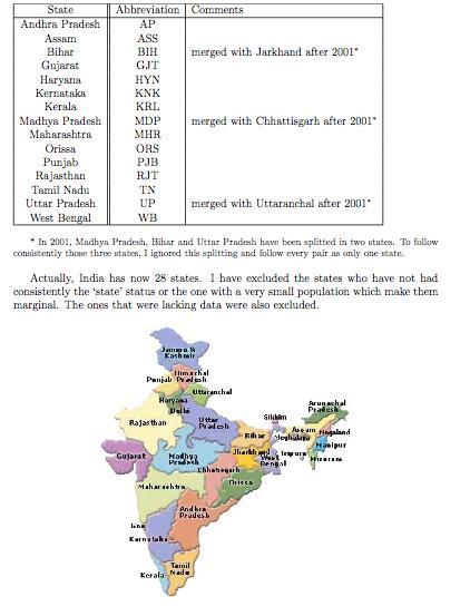
49 48