IEOR E4602: Quantitative Risk Management

Transcription

1 IEOR E4602: Quantitative Risk Management Basic Concepts and Techniques of Risk Management Martin Haugh Department of Industrial Engineering and Operations Research Columbia University References: Chapter 2 of 2 nd ed. of MFE by McNeil, Frey and Embrechts.

2 Outline Risk Factors and Loss Distributions Linear Approximations to the Loss Function Conditional and Unconditional Loss Distributions Risk Measurement Scenario Analysis and Stress Testing Value-at-Risk Expected Shortfall (ES) Standard Techniques for Risk Measurement Evaluating Risk Measurement Techniques Other Considerations 2 (Section 0)

3 Risk Factors and Loss Distributions Notation (to be used throughout the course): a fixed period of time such as 1 day or 1 week. Let V t be the value of a portfolio at time t. So portfolio loss between t and (t + 1) is given by L t+1 := (V t+1 V t ) - note that a loss is a positive quantity - it (of course) depends on change in values of the securities. More generally, may wish to define a set of d risk factors Z t := (Z t,1,..., Z t,d ) so that V t = f (t, Z t ). for some function f : R + R d R. 3 (Section 1)

4 Risk Factors and Loss Distributions e.g. In a stock portfolio might take the stock prices or some function of the stock prices as our risk factors. e.g. In an options portfolio Z t might contain stock factors together with implied volatility and interest rate factors. Let X t := Z t Z t 1 denote the change in values of the risk factors between times t and t + 1. Then have L t+1 (X t+1 ) = (f (t + 1, Z t + X t+1 ) f (t, Z t )) Given the value of Z t, the distribution of L t+1 depends only on the distribution of X t+1. Estimating the (conditional) distribution of X t+1 is then a very important goal in much of risk management. 4 (Section 1)

5 Linear Approximations to the Loss Function Assuming f (, ) is differentiable, can use a first order Taylor expansion to approximate L t+1 : ˆL t+1 (X t+1 ) := ( f t (t, Z t ) + ) d f zi (t, Z t ) X t+1,i i=1 (1) where f -subscripts denote partial derivatives. First order approximation commonly used when X t+1 is likely to be small - often the case when is small, e.g. = 1/365 1 day, and market not too volatile. Second and higher order approximations also based on Taylor s Theorem can also be used. Important to note, however, that if X t+1 is likely to be very large then Taylor approximations can fail. 5 (Section 1)

6 Conditional and Unconditional Loss Distributions Important to distinguish between the conditional and unconditional loss distributions. Consider the series X t of risk factor changes and assume that they form a stationary time series with stationary distribution F X. Let F t denote all information available in the system at time t including in particular {X s : s t}. Definition: The unconditional loss distribution is the distribution of L t+1 given the time t composition of the portfolio and assuming the CDF of X t+1 is given by F X. Definition: The conditional loss distribution is the distribution of L t+1 given the time t composition of the portfolio and conditional on the information in F t. 6 (Section 1)

7 Conditional and Unconditional Loss Distributions If the X t s are IID then the conditional and unconditional distributions coincide. For long time horizons, e.g. = 6 months, we might be more inclined to use the unconditional loss distribution. However, for short horizons, e.g. 1 day or 10 days, then the conditional loss distribution is clearly the appropriate distribution - true in particular in times of high market volatility when the unconditional distribution would bear little resemblance to the true conditional distribution. 7 (Section 1)

8 Example: A Stock Portfolio Consider a portfolio of d stocks with S t,i denoting time t price of the i th stock and λ i denoting number of units of i th stock. Take log stock prices as risk factors so X t+1,i = ln S t+1,i ln S t,i and L t+1 Linear approximation satisfies d ( = λ i S t,i e X t+1,i 1 ). i=1 where ω t,i ˆL t+1 d d = λ i S t,i X t+1,i = V t ω t,i X t+1,i i=1 i=1 := λ i S t,i /V t is the i th portfolio weight. If E[X t+1,i ] = µ and Covar(X t+1,i ) = Σ, then E t [ˆLt+1 ] = V t ω µ and Var t (ˆLt+1 ) = V 2 t ω Σω. 8 (Section 1)

9 Example: An Options Portfolio Recall the Black-Scholes formula for time t price of a European call option with strike K and maturity T on a non-dividend paying stock satisfies C(S t, t, σ) = S t Φ(d 1 ) e r(t t) KΦ(d 2 ) and where: where d 1 = log ( S t K ) + (r + σ 2 /2)(T t) σ T t d 2 = d 1 σ T t Φ( ) is the standard normal distribution CDF S t = time t price of underlying security r = continuously compounded risk-free interest rate. In practice use an implied volatility, σ(k, T, t), that depends on strike, maturity and current time, t. 9 (Section 1)

10 Example: An Options Portfolio Consider a portfolio of European options all on the same underlying security. If the portfolio contains d different options with a position of λ i in the i th option, then L t+1 = λ 0 (S t+1 S t ) d λ i (C(S t+1, t + 1, σ(k i, T i, t + 1) C(S t, t, σ(k i, T i, t))) i=1 where λ 0 is the position in the underlying security. Note that by put-call parity we can assume that all options are call options. Can also use linear approximation technique to approximate L t+1 - would result in a delta-vega-theta approximation. For derivatives portfolios, the linear approximation based on 1 st order Greeks is often inadequate - 2 nd order approximations involving gamma, volga and vanna might then be used but see earlier warning regarding use of Taylor approximations. 10 (Section 1)

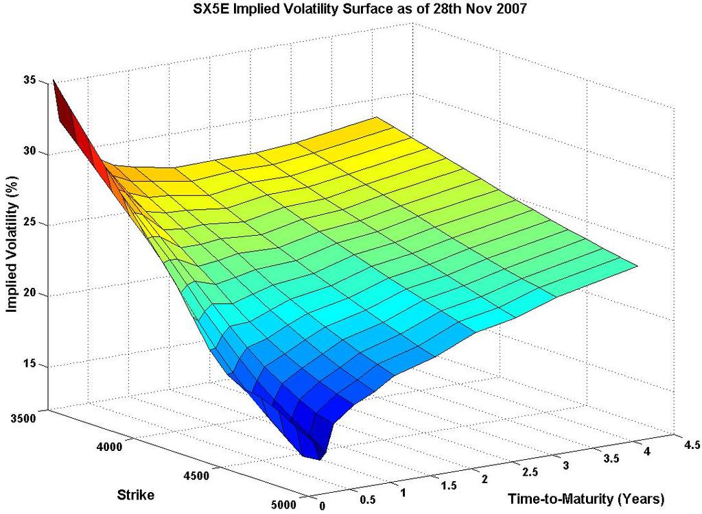
11 Risk Factors in the Options Portfolio Can again take log stock prices as risk factors but not clear how to handle the implied volatilities. There are several possibilities: 1. Assume the σ(k, T, t) s simply do not change - not very satisfactory but commonly assumed when historical simulation is used to approximate the loss distribution and historical data on the changes in implied volatilities are not available. 2. Let each σ(k, T, t) be a separate factor. Not good for two reasons: (a) It introduces a large number of factors. (b) Implied volatilities are not free to move independently since no-arbitrage assumption imposes strong restrictions on how volatility surface may move. Therefore important to choose factors in such a way that no-arbitrage restrictions are easily imposed when we estimate the loss distribution. 11 (Section 1)

12 Risk Factors in the Options Portfolio 3. In light of previous point, it may be a good idea to parameterize the volatility surface with just a few parameters - and assume that only those parameters can move from one period to the next - parameterization should be so that no-arbitrage restrictions are easy to enforce. 4. Use dimension reduction techniques such as principal components analysis (PCA) to identify just two or three factors that explain most of the movements in the volatility surface. 12 (Section 1)

13

14 Example: A Bond Portfolio Consider a portfolio containing quantities of d different default-free zero-coupon bonds. Thei th bond has price P t,i, maturity T i and face value 1. s t,ti is the continuously compounded spot interest rate for maturity T i so that P t,i = exp( s t,ti (T i t)). There are λ i units of i th bond in the portfolio so total portfolio value given by V t = d λ i exp( s t,ti (T i t)). i=1 14 (Section 1)

15 Example: A Bond Portfolio Assume now only parallel changes in the spot rate curve are possible - while unrealistic, a common assumption in practice - this is the assumption behind the use of duration and convexity. Then if spot curve moves by δ the portfolio loss satisfies L t+1 = d i=1 λ i ( e (s t+,t i +δ)(t i t ) e s t,t i (T i t) ) d λ i (s t,ti (T i t) (s t+,ti + δ)(t i t )). i=1 Therefore have a single risk factor, δ. 15 (Section 1)

16 Approaches to Risk Measurement 1. Notional Amount Approach. 2. Factor Sensitivity Measures. 3. Scenario Approach. 4. Measures based on loss distribution, e.g. Value-at-Risk (VaR) or Conditional Value-at-Risk (CVaR). 16 (Section 2)

17 An Example of Factor Sensitivity Measures: the Greeks Scenario analysis for derivatives portfolios is often combined with the Greeks to understand the riskiness of a portfolio - and sometimes to perform a P&L attribution. Suppose then we have a portfolio of options and futures - all written on the same underlying security. Portfolio value is the sum of values of individual security positions - and the same is true for the portfolio Greeks, e.g. the portfolio delta, portfolio gamma and portfolio vega. Why? Consider now a single option in the portfolio with price C(S, σ,...). Will use a delta-gamma-vega approximation to estimate risk of the position - but approximation also applies (why?) to the entire portfolio. Note approximation only holds for small moves in underlying risk factors - a very important observation that is lost on many people! 17 (Section 2)

18 Delta-Gamma-Vega Approximations to Option Prices A simple application of Taylor s Theorem yields C(S + S, σ + σ) C(S, σ) + S C S ( S)2 2 C C + σ S 2 σ Therefore obtain = C(S, σ) + S δ ( S)2 Γ + σ vega. P&L δ S + Γ 2 ( S)2 + vega σ = delta P&L + gamma P&L + vega P&L. When σ = 0, obtain the well-known delta-gamma approximation - often used, for example, in historical Value-at-Risk (VaR) calculations. Can also write P&L δs ( ) S + ΓS 2 S 2 ( ) 2 S + vega σ S = ESP Return + $ Gamma Return 2 + vega σ (2) where ESP denotes the equivalent stock position or dollar delta. 18 (Section 2)

19 Scenario Analysis and Stress Testing Stress testing an options portfolio written on the Eurostoxx (Section 2)

20 Scenario Analysis and Stress Testing In general we want to stress the risk factors in our portfolio. Therefore very important to understand the dynamics of the risk factors. e.g. The implied volatility surface almost never experiences parallel shifts. Why? - In fact changes in volatility surface tend to follow a square root of time rule. When stressing a portfolio, it is also important to understand what risk factors the portfolio is exposed to. e.g. A portfolio may be neutral with respect to the two most important" risk factors but have very significant exposure to a third risk factor - Important then to conduct stresses of that third risk factor - Especially if the trader or portfolio manager knows what stresses are applied! 20 (Section 2)

21

22 Value-at-Risk Value-at-Risk (VaR) the most widely (mis-)used risk measure in the financial industry. Despite the many weaknesses of VaR, financial institutions are required to use it under the Basel II capital-adequacy framework. And many institutions routinely report VaR numbers to shareholders, investors or regulatory authorities. VaR is calculated from the loss distribution - could be conditional or unconditional - could be a true loss distribution or some approximation to it. Will assume that horizon has been fixed so that L represents portfolio loss over time interval. Will use F L ( ) to denote the CDF of L. 22 (Section 2)

23 Value-at-Risk Definition: Let F : R [0, 1] be an arbitrary CDF. Then for α (0, 1) the α-quantile of F is defined by q α (F) := inf{x R : F(x) α}. If F is continuous and strictly increasing, then q α (F) = F 1 (α). For a random variable L with CDF F L ( ), will often write q α (L) instead of q α (F L ). Since any CDF is by definition right-continuous, immediately obtain the following result: Lemma: A point x 0 R is the α-quantile of F L if and only if (i) F L (x 0 ) α and (ii) F L (x) < α for all x < x 0. Definition: Let α (0, 1) be some fixed confidence level. Then the VaR of the portfolio loss at the confidence interval, α, is given by VaR α := q α (L), the α-quantile of the loss distribution. 23 (Section 2)

24 VaR for the Normal Distributions Because the normal CDF is both continuous and strictly increasing, it is straightforward to calculate VaR α. So suppose L N(µ, σ 2 ). Then where Φ( ) is the standard normal CDF. VaR α = µ + σφ 1 (α) (3) This follows from previous lemma if we can show F L (VaR α ) = α - but this follows immediately from (3). 24 (Section 2)

25 VaR for the t Distributions The t CDF also continuous and strictly increasing so again straightforward to calculate VaR α. So let L t(ν, µ, σ 2 ), i.e. (L µ)/σ has a standard t distribution with ν > 2 degrees-of-freedom (dof). Then VaR α = µ + σtν 1 (α) where t ν is the CDF for the t distribution with ν dof. Note that now E[L] = µ and Var(L) = νσ 2 /(ν 2). 25 (Section 2)

26 Weaknesses of VaR 1. VaR attempts to describe the entire loss distribution with just a single number! - so significant information is lost - this criticism applies to all scalar risk measures - one way around it is to report VaR α for several values of α. 2. Significant model risk attached to VaR - e.g. if loss distribution is heavy-tailed but a light-tailed, e.g. normal, distribution is assumed, then VaR α will be severely underestimated as α A fundamental problem with VaR is that it can be very difficult to estimate the loss distribution - true of all risk measures based on the loss distribution. 4. VaR is not a sub-additive risk measure so that it doesn t lend itself to aggregation. 26 (Section 2)

27 (Non-) Sub-Additivity of VaR e.g. Let L = L 1 + L 2 be the total loss associated with two portfolios, each with respective losses, L 1 and L 2. Then q α (F L ) > q α (F L1 ) + q α (F L2 ) is possible! An undesirable property as we would expect some diversification benefits when we combine two portfolios together. Such a benefit would be reflected by the combined portfolio having a smaller risk measure than the sum of the two individual risk measures. Will discuss sub-additivity property when we study coherent risk measures later in course. 27 (Section 2)

28 Advantages of VaR VaR is generally easier to estimate: True of quantile estimation in general since quantiles are not very sensitive to outliers. - not true of other risk measures such as Expected Shortfall / CVaR Even then, it becomes progressively more difficult to estimate VaR α as α 1 - may be able to use Extreme Value Theory (EVT) in these circumstances. But VaR easier to estimate only if we have correctly specified the appropriate probability model - often an unjustifiable assumption! Value of that is used in practice generally depends on the application: For credit, operational and insurance risk often on the order of 1 year. For financial risks typical values of are on the order of days. 28 (Section 2)

29 Expected Shortfall (ES) Definition: For a portfolio loss, L, satisfying E[ L ] < the expected shortfall at confidence level α (0, 1) is given by ES α := 1 1 α 1 α q u (F L ) du. (4) Relationship between ES α and VaR α is therefore given by ES α := 1 1 α 1 α VaR u (L) du - so clear that ES α (L) VaR α (L). 29 (Section 2)

30 Expected Shortfall (ES) A more well known representation of ES α (L) holds when F L is continuous: Lemma: If F L is a continuous CDF then ES α := E [L; L q α(l)] 1 α = E [L L VaR α ]. (5) Proof: See Lemma 2.13 in McNeil, Frey and Embrechts (MFE). Expected Shortfall also known as Conditional Value-at-Risk (CVaR) - when there are atoms in the distribution CVaR is defined slightly differently - but we will continue to take (4) as our definition. 30 (Section 2)

31 Example: Expected Shortfall for a Normal Distribution Can use (5) to compute expected shortfall of an N(µ, σ 2 ) random variable. We find ES α = µ + σ φ (Φ 1 (α)) 1 α where φ( ) is the PDF of the standard normal distribution. (6) 31 (Section 2)

32 Example: Expected Shortfall for a t Distribution Let L t(ν, µ, σ 2 ) so that L := (L µ)/σ has a standard t distribution with ν > 2 dof. Then easy to see that ES α (L) = µ + σes α ( L). Straightforward using direct integration to check that ES α ( L) = g ν (tν 1 (α)) 1 α ( ν + (t 1 ν (α)) 2 ) ν 1 (7) where t ν ( ) and g ν ( ) are the CDF and PDF, respectively, of the standard t distribution with ν dof. Remark: The t distribution is a much better model of stock (and other asset) returns than the normal model. In empirical studies, values of ν around 5 or 6 are often found to fit best. 32 (Section 2)

33 The Shortfall-to-Quantile Ratio Can compare VaR α and ES α by considering their ratio as α 1. Not too difficult to see that in the case of the normal distribution ES α VaR α 1 as α 1. However, in the case of the t distribution with ν > 1 dof we have ES α ν VaR α ν 1 > 1 as α (Section 2)

34 Standard Techniques for Risk Measurement 1. Historical simulation. 2. Monte-Carlo simulation. 3. Variance-covariance approach. 34 (Section 3)

35 Historical Simulation Instead of using a probabilistic model to estimate distribution of L t+1 (X t+1 ), we could estimate the distribution using a historical simulation. In particular, if we know the values of X t i+1 for i = 1,..., n, then can use this data to create a set of historical losses: { L i := L t+1 (X t i+1 ) : i = 1,..., n} - so L i is the portfolio loss that would occur if the risk factor returns on date t i + 1 were to recur. To calculate value of a given risk measure we simply assume the distribution of L t+1 (X t+1 ) is discrete and takes on each of the values L i w.p. 1/n for i = 1,..., n, i.e., we use the empirical distribution of the X t s. e.g. Suppose we wish to estimate VaR α. Then can do so by computing the α-quantile of the L i s. 35 (Section 3)

36 Historical Simulation Suppose the L i s are ordered by L n,n L 1,n. Then an estimator of VaR α (L t+1 ) is L [n(1 α)],n where [n(1 α)] is the largest integer not exceeding n(1 α). Can estimate ES α using ẼS α = L [n(1 α)],n + + L 1,n. [n(1 α)] Historical simulation approach generally difficult to apply for derivative portfolios. Why? But if applicable, then easy to apply. Historical simulation estimates the unconditional loss distribution - so not good for financial applications! 36 (Section 3)

37 Monte-Carlo Simulation Monte-Carlo approach similar to historical simulation approach. But now use some parametric distribution for the change in risk factors to generate sample portfolio losses. The (conditional or unconditional) distribution of the risk factors is estimated and m portfolio loss samples are generated. Free to make m as large as possible Subject to constraints on computational time. Variance reduction methods often employed to obtain improved estimates of required risk measures. While Monte-Carlo is an excellent tool, it is only as good as the model used to generate the data: if the estimated distribution of X t+1 is poor, then Monte-Carlo of little value. 37 (Section 3)

38 The Variance-Covariance Approach In the variance-covariance approach assume that X t+1 has a multivariate normal distribution so that X t+1 MVN (µ, Σ). Also assume the linear approximation ( ˆL t+1 (X t+1 ) := is sufficiently accurate. Then can write f t (t, Z t ) + ) d f zi (t, Z t ) X t+1,i i=1 ˆL t+1 (X t+1 ) = (c t + b t X t+1 ) for a constant scalar, c t, and constant vector, b t. Therefore obtain ) ˆL t+1 (X t+1 ) N ( c t b t µ, b t Σb t. and can calculate any risk measures of interest. 38 (Section 3)

39 The Variance-Covariance Approach This technique can be either conditional or unconditional - depends on how µ and Σ are estimated. The approach provides straightforward analytically tractable method of determining the loss distribution. But it has several weaknesses: risk factor distributions are often fat- or heavy-tailed but the normal distribution is light-tailed - this is easy to overcome as there are other multivariate distributions that are also closed under linear operations. e.g. If X t+1 has a multivariate t distribution so that X t+1 t (ν, µ, Σ) then ) ˆL t+1 (X t+1 ) t (ν, c t b t µ, b t Σb t. A more serious problem is that the linear approximation will often not work well - particularly true for portfolios of derivative securities. 39 (Section 3)

40 Evaluating Risk Measurement Techniques Important for any risk manger to constantly evaluate the reported risk measures. e.g. If daily 95% VaR is reported then should see daily losses exceeding the reported VaR approximately 95% of the time. So suppose reported VaR numbers are correct and define Y i := { 1, Li VaR i 0, otherwise where VaR i and L i are the reported VaR and realized loss for period i. If Y i s are IID, then n Y i Binomial(n,.05) i=1 Can use standard statistical tests to see if this is indeed the case. Similar tests can be constructed for ES and other risk measures. 40 (Section 3)

41 Other Considerations Risk-Neutral and Data-Generating (Empirical) Probability Measures. Data Risk. Multi-Period Risk Measures and Scaling. Model Risk. Data Aggregation. Liquidity Risk. P&L Attribution. 41 (Section 4)