BASIC IS-LM by John Eckalbar

Size: px

Start display at page:

Download "BASIC IS-LM by John Eckalbar"

Alban Powell
5 years ago
Views:

1 BASIC IS-LM by John Eckalbar The idea here is to get some flavor for the way M works in an IS-LM model. We are going to look at the simplest possible case: There are 3 items getting traded: money, final goods, and bonds. There are 3 sectors: households, firms, government. at t. There is no foreign sector, no labor market, prices are exogenous at P, real taxes are fixed Goods market 1. Households demand real consumption goods, c, according to the linear equation c = a + b(y - t), where y is real income and a and b are fixed positive constants, with b < 1 2. Firms demand investment goods according to: i = d - f r, where i is planned real investment, r is the nominal interest rate, and d and f are fixed positive constants. 3. Government buys real output of g and collects real taxes of t. 4. The goods market is in equilibrium when y = c + i + g, or y = a + b(y - t) + d - f r + g, or y(1 - b) = a - b t + d - f r + g, or y = (a - b t + d - f r + g)/(1 - b), or r = (a - b t + d + g)/f -y(1 - b)/f Define the IS curve to be the set of all (y, r) points at which r = (a - b t + d + g)/f - y(1 - b)/f...that is, the set of all r and y points at which the goods market clears. A plot of IS with relevant intercepts and slopes is shown here. Can you list all sources of IS-curve shift? Can you show how IS would shift with changes in g, etc.? If we are at a point like A, are goods in excess demand or excess supply?

2 LM Let nominal money demand be given by Md = k P y + h - j r, where k, h, j > 0 and P is the exogenous price level. Let Ms be the money supply. Money demand equals money supply when: y = (Ms - h + j r)/ (k P) r = (h - Ms)/j + (k P y)/j Define LM to be the set of (y, r) points where Ms = Md. Then LM is as shown below: Again: identify all the ways this can shift. If we are at a point like B, is Md > Ms?

3 The whole story The equilibrium is at ye and re. Be sure you can explain all the factors that would make ye and re change. Where would be move if we happened to be at point X? (Ans.: Assume that if c + i + g > y, then y increases, and if Md > Ms, then r increases. That will let you plot out the vector field...more on this in class.) For what it s worth, though you don t have to be able to derive this. Could you fill this in? Event y r g t M P k h..

4 The big feature of IS-LM is that ye may not be at full employment. If aggregate demand, c + i + g, is low, then ye may well be less than full employment output, yfe. Some have argued that if ye < yfe, then wages will fall...prices will fall...lm will shift right (check this with the equations)...and ye will rise, BUT: 1. Where is the labor market in this model? And how do we treat this analytically? Always be suspect of discussing how a model reacts when something changes that is not explicitly in the model. 2. If P is falling, won t that lead to expectations of further price reductions, and won t this prompt traders to delay spending on c and i, thus causing IS to fall? 3. People with nominally fixed debts may go bankrupt...what does that mean? In any case, the story won t unfold (i.e., falling prices won t lead to full employment) if: 1. Wages are rigid. 2. Md has an interest inelastic segment (liquidity trap). Here s the deal on that: I ll show why in class, but the punch line is that if Ms increases or P falls, LM will slide right, but if IS is down low on the left hand/flat part of LM, then ye will not increase, so monetary policy won t do much.

5 3. If investment demand is interest inelastic, IS will be vertical, and again falling P or rising M won t increase ye, as you see below. These are the so-called Keynesian cases, though Keynes himself would not be happy seeing his name attached to the term.

What does IS-LM have to say about velocity? By definition, V = P y/ms, so anything that affects P, y, and/or Ms should affect velocity, unless there is some special case at work.

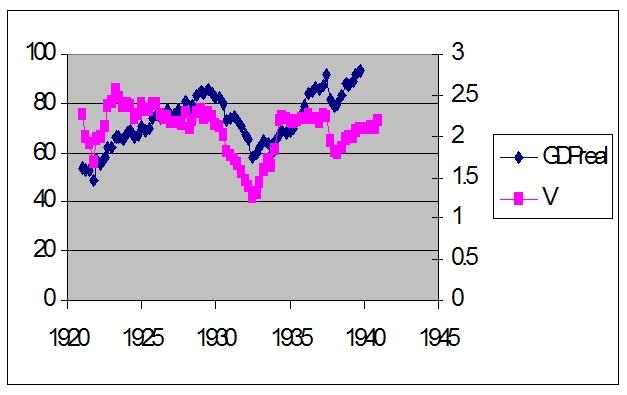
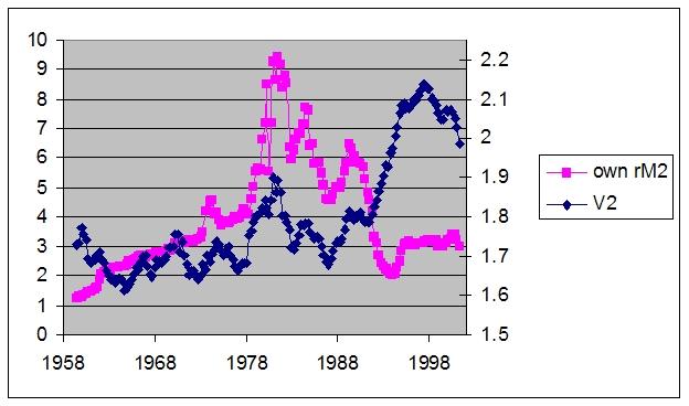
6 What does IS-LM have to say about velocity? By definition, V = P y/ms, so anything that affects P, y, and/or Ms should affect velocity, unless there is some special case at work. For example, if g increased, IS would shift right and ye would increase, so with P and Ms fixed, V would rise. In a sense, IS-LM could be thought of as variable velocity quantity theory, though you don t gain much by thinking of it that way... In effect, V is not particularly interesting in an IS-LM framework. In case you re curious, you can solve to get: V = Note that if a, d, or g increases, V increases. In general, anything that shifts IS to the right will cause V to increase and r to increase...so you might see V and r moving in parallel when IS moves. But if changes in the money demand parameters h, k, or j cause LM to shift, V and r will move in opposite directions. The graph below shows something interesting. We fit an equation for money demand from the period 1959 to 1990 we get M2 = *gdp *OpCost M2, and it gives a good fit over that period. Here is the result. See how actual money demand is a good fit with the equation until about (Though the equation itself is very primitive.) If we continued to use that equation to the period just after 1990, it wanders way off the actual track of M. So it looks like Md shifted or went unstable in about This is about when the Fed quit targeting M2...and this is the reason.

7 More recently, the fitted and actual lines have re-connected somewhat, but the past year or so has shown another break ( FITS1 is the fitted level of money demand according to the equation.):

8 Velocity, Money Demand, and Policy Since V is defined as PQ/M, MV will always equal PQ. This is not a theory, it is a definition. From time to time we will call PQ nominal income or Y. If V were a constant, monetary policy aimed at setting the level of M would (if it succeeded in setting the desired level of M...a big IF) completely determine the value of Y. Note that the split between P and Q is not determined, just the product Y = PQ. In this circumstance there would probably be a theory about how, over the long run, with Q moving roughly along its long run growth path, M growth would determine P growth, or inflation. (With V constant, % M = % P + % Q, so % M - % Q = % P...money growth minus real growth equals inflation. The Fed could pick a target long run average inflation rate, and then set % M to fit the above equation and meet the inflation objective.) Short run effects on Q could also be studied, but extra equations would be necessary. In this circumstance (i.e., if V were constant) people working at the Fed may or (surprisingly) may not need to pay a lot of attention to M. Consider this: Suppose we have a different-looking theory of PQ. Suppose PQ is determined by nominal Aggregate Demand (AD), which consists of the levels of demand coming from C, I, G, and NX (net exports). Suppose further that major components of C and I are dependent upon the interest rate. We could write AD(r) = Y = PQ and use some derivative of the C + I + G + NX and 45-degree line model to determine equilibrium Y, which would depend upon r. This is really just an IS curve when drawn in (r,y)-space Now if the Fed controlled r, it would control Y, even if it paid no attention to M. In theory, nothing whatever rules out having both V constant and AD(r). Both of these models could be true at the same time. All that is needed is a vertical LM curve with a normal IS. If so, when the Fed adjusts r to move on IS and change Y, it is forced to change M according to MV = PQ = Y. Both theories are simultaneously true, and arguments about which is correct are pointless. Note that if V were not constant, but were highly predictable, essentially the same monetary policy could be followed. That is, if V were known to be autonomously growing (i.e., growing due to changes in the efficiency of the payments system, rather than, say, to changes in interest rates) at a rate of, say, 3% per year, the Fed could use % M + % V = % P + % Q. This was Friedman s advice in the late 60s and 70s...For example, if long run % Q = 2.5, % V = 3, and target inflation is 1, then the Fed s monetary policy rule would be to set % M = =.5. Remember from the Cambridge version of the quantity theory that if V is constant and money demand equals money supply, then M = kpq = ky, where k is a constant. This means, and this is important, M demand is a fixed ratio, k, of PQ or Y. And this means that money demand is not a function of interest rates, r. If money demand were a function of r, Md(r), then since in equilibrium V = PQ/Ms = PQ/Md(r)...V would be a function of r...and not a constant. Suppose money demand is a stable function of r and Y in the sense that when money demand equals money supply, we can write M = ky - jr +, where k and j do not vary over time and the error term is small enough to be ignored. This would give us the usual LM curve. If we also had the usual IS curve that derives from a stable AD(r) function, then again, monetary policy could focus either on M or r. If the Fed wanted Y = Y fe = AD(r fe ), where r fe is the interest rate that sets AD(r) = Y fe, the Fed could target M at ky fe - j r fe. But wouldn t it be simpler for the Fed to simply target r at r fe, buying and selling bonds as needed to keep r = r fe. Then markets would automatically move M to ky fe - j r fe. (Keynes has some thoughts on this that we will explore later.) With regard to velocity, if M = ky - j r, V = Y/(kY - jr). Other things (like C, I,

9 G, NX) being equal, you would expect to see V positively correlated with r. In fact this is the way things looked for M1 until about 1980 and for M2 until about If V were wildly erratic and unpredictable, then there would be little to no point in trying to control M., since M would not correlate with any of the Fed s ultimate objectives. In that case, the Fed might as well target the number of goats in Bidwell Park. If instead, the Aggregate Demand had some predictable reaction to r, the Fed would simply target r, and adjust the target as necessary to nudge Y in the desired direction. In fact, when it was clear that V1 was becoming unpredictable starting in the early 80s, the Fed finally gave up on targeting M1. V2 lost its historical relation to r in about 1990, and the Fed quickly gave up on it as well. There is now some evidence that V MZM has a stable relationship with r (actually its opportunity cost), but there is relatively little interest in firmly targeting MZM.

10 IS-LM and Friedman The figure below shows a graphical method of deriving the LM curve. The above figures show what might be called the standard case. Money demand is interest elastic, while Ms is interest inelastic. The end result is that LM has a positive slope. See if you can use the graph to show that if the Md curves were interest inelastic, then LM would be vertical, or interest inelastic. Using the equations from earlier, we see that if the interest elasticity of Md is 0, then j = 0 and the LM is vertical...assuming that Ms also has a zero interest elasticity. If so, the LM would be vertical in this case. What would a vertical LM imply about monetary vs. fiscal policy? Draw some pictures and figure it out. This is important stuff.

11 So if you viewed the world through IS-LM lenses, you would believe that the effectiveness of monetary vs. Fiscal policy depends critically upon the slope of LM. As we look closely at this, what we find is that LM have it s normal upward slope if either Md or Ms is interest elastic. Let us look into these in turn. Interest elasticity of Md. We will look at the theory behind two different reasons for believing that Md is interest elastic. Speculative Money Demand under Certainty Assume a consol pays $1 per year forever. It s market value at time t will be 1/rt, where rt is the interest rate at time t. Any on trader s expected gain from holding a consol for one year would be A little arithmetic shows that We take any one trader s interest expectations as a given and ask whether she/he would want to hold money or bonds at various values of rt. For example, suppose you expected the interest rate to be 5% in one year. Then, and if rt >.476 you want to hold bonds, while if rt <.0476 you want to hold money for speculative purposes. In this case.0476 is the critical interest rate. Your money demand curve will look like this (at left).

12 At the same time, I might expect interest rates to be 7% in one year. Then my critical interest rate is.07/1.07 =.065. In the above graph, me has high interest rate expectations, her has low ones, and you is in the middle. The market-wide total speculative demand curve on the right is the horizontal sum of the three on the left. With many traders, the curve will be smoother in appearance. Of course, all of this is static. We aren t analyzing how interest rate expectations evolve over time or what determines them. This much should be obvious though: 1. There are speculative reasons for holding money. 2..The money demand curve is interest elastic. 3. When peoples interest expectations rise, the money demand curve shifts up or to the right, and this will cause LM to shift up/right. 4. Actual rates depend strongly upon expectations, and expectations depend upon rates. The interest elasticity of transactions demand: Baumol model. Suppose that over a year-long interval you are going to spend a total of T dollars in a steady stream. You have the option of holding cash, which pays no interest or holding, say, a bond that returns r per dollar per year. Every time you go to the broker to get cash, you incur a transaction cost of b dollars per visit. You could withdraw all your cash on January 1 and save a lot on transactions costs by only having to go to the broker once per year, but then you would have to hold an average of T/2 dollars during the year and you interest opportunity cost would be high...it would be rt/2 if we ignore compounding. To save interest opportunity cost you could withdraw money quite often, but then your transaction costs, b, would be high. How do you manage your cash withdrawls? We can figure this out as follows: Let C be the size of each cash withdrawl and assume that all withdrawls are of equal size. It follows that you need to make T/C withdrawls per year, so your total transaction cost will be bt/c. Your average money holding will be C/2, so your annual interest opportunity cost will be rc/2. So your total cost of ready cash is. What you want to do is pick C so as to minimize this total. The technique is to take the derivative of with respect to C, set the result equal to zero, and solve for C. The value of the derivative we seek is. Setting this equal to zero and solving for C we have the optimal cash withdrawl given by

13 . This is the famous square root rule. Since C/2 is in a sense one s average money demand, this equation tells us about the interest elasticity of money demand. Note that if r increases, the optimal C declines. Note also that if b or T increases, money demand rises. Since T will tend to correlate with a person s income, this seems to make one believe that, in our more common notation, Md = f(y, r).

14 Interest Elasticity of Money Supply Even if Md is interest inelastic, if Ms is interest elastic so is LM. I ll give a quick graph and we will explore details in a minute. The figure below shows Md as completely interest inelastic, with Ms as elastic. Note that this give LM the usual shape. Why might Ms be interest elastic? Maybe when r increases people switch from demand deposits to time deposits, and this frees up reserves, or maybe currency flows into the banking system, and this gives banks reserves and allows them to increase loans and deposits.one way to explore this is via the money multiplier. Here s how: 1. M2 = C + D + T 2. C = cr M2 3. T = t M2 4. H = R + C 5. R = RR + XR 6. RR = rr D 7. XR = xr D where C is currency held by the public, D is demand deposits, and T is time deposits Where the currency ratio, cr, is a positive constant Where t, the time deposit ratio, is a positive constant. We assume that 1 - cr - t > 0 Where H is high powered money, with R being bank vault cash or bank reserve deposits at the Fed. H is either reserves or cash, which could be reserves if the public decided to put the cash in the bank. Reserves are either required reserves, RR, or excess reserves, XR Where rr is the required reserve ratio. Time deposits don t have required reserves.

15 If you substitute into equation 4, you get xr is the banking systems excess reserve demand ratio. The idea is that the Fed influences H and rr, while the banks influence xr, and the public determines cr and t. The resulting money supply is end result of all of their actions. To illustrate: Open market purchases of bonds by the Fed will increase H, and this will increase M2, if everything else remains constant. If the Fed increases rr, then M2 should fall, since (1 - c - t) > 0. If the banks want to hold more excess reserves, i.e., xr increases, then mm falls and so does M2 with everything else held constant. When would xr increase? Maybe when interest rates are low, hence the interest elasticity of Ms. If t increases, mm will rise and so will M2. This might happen when interest rates rise hence the interest elasticity of Ms. Exercise: What happens when cr increases? All of these factors point to the interest elasticity of Ms, and therefor a positive slope for LM. Question: How would we use IS-LM if the Fed followed a policy of adjusting Ms in whatever way necessary to hold r = r0?

16 Monetary vs. Fiscal Policy One of the problems with IS-LM as it is conventionally used is that it allows one to ask and get answers to nonsense questions. For example, it is possible to use IS-LM to answer a question like, What happens if we have an increase in g? Or what happens if we have an increase in M? (These may not seem like crazy questions, but they are.) And IS-LM allows us to draw an artificially solid line between monetary and fiscal policy. Why are these nonsense questions? Think of [ g] as an event. We can ask (inside IS- LM), what happens following this event. But this sort of event can never happen. Like every other entity, the government has a budget constraint. The constraint looks like this: g = t + Pb B + M This says that the government s spending must be financed somehow...either by taxes, t, bond sales to the public that bring in Pb B, where Pb is the price of bonds and B is the quantity of bonds held by the public, or by printing money, M. Given this, we can ask about the effects of events like: [ g, t] or [ g, Pb B] or [ g, M], but [ g] makes no sense. This is a big deal. I can t predict what an increase in g will do unless I know how it will be financed.. Here s how all this can give rise to an artificial distinction between monetary and fiscal policy. Consider a few T accounts: 1. The Fed buys bonds from the public. The event is [ M and B ]. This is monetary policy. Since Deposits and Reserves initially increase equally, there will be excess reserves, XR, which prompt banks to make more loans and expand the money supply. So we have M rising and no change in g...looks like monetary policy. 2. What if the treasury increased t and spent the money buying a 747 from Boeing (the public sector)? The event is [ g and t]. Here s what the accts would look like. The financing is above the dashed line and the spending is below. This looks like fiscal policy, since we have g and t changing, but no change in M and not much commotion in financial markets.

17 3. What if the treasury increases g and sold bonds to the public to finance the purchase? The event is [ g and B]. The financing is above the line and the spending is below the line. Note that this involves an increase in g and no change in M, but there will be considerable monetary commotion due to the bond sale. 4. What if the treasury spent more on g by simply running down its deposits at the Fed? The event is [ g and M]. The T acct is just the items below the line in the above figure. This time we get an increase in g and an increase in M. Is this monetary or fiscal policy? 5. Finally, what if the Fed bought a B747 or a new computer system? Is that monetary of fiscal policy? As interest rates drop toward zero here and in Japan, people worry about the ability of Monetary policy aimed at reducing r...one of the options is to have the central bank buy things other than very short T-bills...the further one goes from t-bills, the closer monetary policy comes to being fiscal policy. Do you see now why it isn t proper to ask about the effect of an increase in g with no discussion of financing?

18 The old template was: fiscal change g [ g] change t [ t] Monetary OMO Change discount rate Change reserve req...[ M] but I like:

Economics 102 Discussion Handout Week 14 Spring Aggregate Supply and Demand: Summary

Economics 102 Discussion Handout Week 14 Spring 2018 Aggregate Supply and Demand: Summary The Aggregate Demand Curve The aggregate demand curve (AD) shows the relationship between the aggregate price level