A BOND MARKET IS-LM SYNTHESIS OF INTEREST RATE DETERMINATION

Transcription

1 A BOND MARKET IS-LM SYNTHESIS OF INTEREST RATE DETERMINATION By Greg Eubanks ABSTRACT: This article fills the gaps left by leading introductory macroeconomic textbooks on how the interest rate gets determined in a closed economy. Leading textbooks offer a simple and incomplete explanation of interest rate determination with a focus on the loanable funds market (IS) and the market for money (LM). The bond market and the market for balances also play an important role in determining the interest rate. When we add these additional markets to the IS-LM analysis, we can get a clearer picture of the causation that changes the interest rate and the accompanying monetary flows. TABLE OF CONTENTS: PREREQUISITES 1.0 THE CIRCULAR FLOW 2.0 INVESTMENT 3.0 AUTONOMOUS EXPENDITURE 4.0 COORDINATING SAVINGS AND INVESTMENT 5.0 MONEY SUPPLY AND DEMAND 6.0 VELOCITY 7.0 THE MARKET FOR BALANCES 8.0 THE BOND MARKET 9.0 SAVINGS, INVESTMENT AND THE BOND MARKET 10.0 THE IS-LM MODEL 11.0 ECONOMIC FLUCTUATIONS 12.0 THE NATURE OF DEBT PREREQUISITES: AGGREGATE SUPPLY AND DEMAND; THE INCOME-EXPENDITURE MODEL The Keynesian general theory of macroeconomics sets out to explain how a closed, two sector, fixed-price economy works. It is a general theory because it can be used to describe a national economy or the world economy. The Keynesian general theory assumes that the aggregate supply curve is perfectly elastic up to the full employment level of output. The price level

2 below the full employment level is decided by the height of the aggregate supply curve. With a perfectly elastic supply curve, the equilibrium level of output is determined solely by aggregate expenditure. Therefore, to know what the equilibrium level of output is, we need to know what determines aggregate expenditure. In the simple Keynesian model of a two sector economy, what determines total aggregate expenditure is the amount of consumption and investment spending in the economy. The assumptions for the aggregate supply curve are that the level of technology and the efficiency and depreciation of capital is held constant. The aggregate demand curve in relation to the aggregate supply curve is vertical because demand depends only on expenditure and not on the price level. This article assumes readers have had introductory macroeconomics 101 and that the reader is familiar with the income-expenditure model covered in macroeconomic textbooks by leading authors like McEachern, Mankiw or Mishkin. 1.0 THE CIRCULAR FLOW The circular flow shows a 2 sector closed economy, meaning there is no foreign trade sector. There will only be 3 assets in this economy: Bonds, money, and GDP. There is no formal banking sector in this economy, making the reality of this model limited. Further limiting the reality of this model is our assumptions of no exchange rates and all prices are fixed, except for the price of money which is the interest rate. These assumptions help to simplify our analysis and allows us to focus on the exchanges between our actors. Also in our model, there is no government agency that taxes and spends. The only government agency in our model is the central bank called the Federal Reserve. Further analysis of the government and trade sectors can always be added in later once we understand how our basic model works. The circular

3 flow model in Fig. 1, illustrates the economic transactions that occurs between households, firms, and the central bank (Fed) in our closed economy. 2.0 INVESTMENT To avoid the terminological problems of saving and investment, economists make a clear distinction between them. By investment we do not mean buying stocks, bonds, or other financial assets, to an economist this is savings. Investment consists of spending on 1) Capital, such as new factories or machinery. 2) Labor and 3) Inventory. Inventory investment is when firms add finished goods to their warehouses. It should be noted here that investors issue bonds to borrow the funds need for planned investment only. Investors do not borrow funds to make unplanned inventory investment. Unplanned inventory investment is assumed to be a purchase by the firm from itself and is counted as expenditure by the firm. Investment decisions are considered more on future forecasts of the return on investment rather than the current levels of income and output in the economy. Investment is determined by 1) Profitable investment opportunities and 2) The cost of borrowing, which is the interest rate. Another possible determinate of investment would be the amount of available funds investors can borrow. After all it would seem that investors cannot borrow more than savers have dedicated to saving. But investors can get around this obstacle because in our model we have a central bank in which it has the authority to create an unlimited amount of money, and through the process of dissaving (which will be covered later), investors can get a hold of the extra funds needed to make their investments, allowing investors to borrow more funds than savers have to offer. This is why investment in our model is assumed to be autonomous with respect to income. If investors could not borrow more funds than savers had to loan, then investment would be dependant on income. And since investment expenditure is what allows income and output to increase, the economy would be stuck at equilibrium without the access to the additional funds. It should be noted here that when investors make any investments in capital, labor or inventories, those investments only add to the economies capacity for output or the replacement of worn out capital and do not add to next period s income and output. We should make notice of the ever increasing debt in the income-expenditure model. When the economy is at equilibrium and stays at equilibrium year after year, debt from investments accumulate. This means that the amount of bonds issued year after year keeps growing. So if the amount of bonds issued in a year is $0.2 trillion, after 10 years at

4 equilibrium, the amount of debt is now $2 trillion. 3.0 AUTONOMOUS EXPENDITURE What exactly allows expenditure to become autonomous and greater than income? When discussing investment demand, we stated that savings is limited to the amount of income households receive and the amount they spend on consumption. Savers can allocate their savings into bonds and/or they may hoard it into speculative balances. The amount that savers allocate to bonds is the amount of funds investors receive for investment expenditure. If the economy is in equilibrium where S=I, and investors want more funds than savers have devoted to bonds making I>S, those funds can come from two sources. Those funds can come from saver's speculative balances, or from the central bank (Fed). In our circular flow model, it is possible for the Fed to buy bonds directly from investors, but it is standard procedure to assume that the Fed buys bonds from savers, who then turn around and buys bonds from investors. When the Fed buys any bonds, it increases the money supply and this is called a monetary expansion. When savers purchase more bonds than their income and savings will allow, this is called dissavings. Dissavings adds to expenditure. Through dissavings, savers can reduce the amount of funds they are holding in speculative balances and buy bonds, or savers can liquidate previously purchased bonds from previous periods of savings to buy new bonds from investors at more favorable rates. Remember savings is a yearly flow, while bonds may be accumulated from previous years. When savers liquidate previously purchased bonds, the Fed buys those bonds and savers may very well earn capital gains. This purchase from the Fed increases the money supply and this money goes into savers speculative balances. If we assume that savers want to purchase bonds from investors instead of holding the extra money in speculative balances, savers will try to get rid of these excess money balances by buying bonds. So what limits the amount of additional bonds savers can buy? This depends on the savers wealth, their accumulated assets of both bonds and speculative balances. Savers cannot purchase more bonds than their available resources will allow. So in summary, investors can attain additional funds greater than the funds savers devote to bonds from their incomes. The sources of the funds come from the Fed by the process of a monetary expansion or from savers by the process of dissavings. Fig. 4.5 shows how funds, starting with the Fed, get handed from one actor to another, where (>) means "money flows to". Fig. 4.5 Central Bank (Fed)> bond market between savers and the Fed>

5 savers> bond market between savers and investors> investors> expenditure> output (income)> savings> savers. 4.0 COORDINATING SAVINGS AND INVESTMENT The income-expenditure model concludes that the economy will be in equilibrium when planned investment equals realized investment, and this is a true statement. But investment is only one half of the S=I equation. When the economy is in equilibrium, planned savings is matched by planned investment. Equilibrium is determined by the plans of both savers and investors. For instance let s assume that the economy is in equilibrium and there is a change in planned savings. If savers increase their demand for speculative balances, this will reduce the amount of funds they devote to bonds. With a change in savings, planned savings is now less than planned investment, assuming there is no change in the plans of investors. Here investors must make inventory investments and the equilibrium level of income must decrease until planned savings again matches planned investment. Likewise, the same change in equilibrium income may happen from a change in investment. Let's return to the same equilibrium level we began with. If investors decrease the amount of investment they plan to spend, this change in investment makes planned investment less than planned savings, and again investors must make inventory investments and the equilibrium level of income must decrease until planned savings equals planned investment. Now finally let's consider a change in the equilibrium level of income in the opposite direction when the plans of investors cause equilibrium income increases. We start again at equilibrium. When investors increase the amount of investment they plan to spend, this makes planned investment greater than planned savings. Firms must reduce their inventories and the equilibrium level of income must increase until planned savings equals planned investment. Notice here that a change in the plans of investors is what causes the equilibrium level of income to increase and not a change in the plans of savers. This is because planned savings cannot become greater than planned investment since savings is dependant on investment. Remember we said that investment in the income-expenditure model comes before savings. Now let's take a more detailed look at our first example when savers increased their demand for speculative balances. When savers received their income, they decided to hold more money in speculative balances, reducing the amount of funds they supply to the bond market. This action causes the demand for bonds curve to shift to the left. This action causes the interest rate to rise and reduces the amount of investment

6 investors undertake. This reduction of funds from the bond market essentially draws money out of required transaction balances and increases the velocity of required transaction balances. Since velocity is required to be 1, there is not enough money in circulation to support all the transactions at the current level of income. Therefore, income must decrease to where velocity equals 1. Finally, firms make inventory investments and decrease production and the equilibrium level of income to where planned savings equals planned investment and velocity is equal to 1. This process of adjustment is summarized by the IS-LM model we will be building in a later chapter. To summarize, the equilibrium level of income condition is met when: 1) planned savings equals planned investment, and 2) the velocity of money sufficiently lubricates the economy. In order for the economy to maintain equilibrium, savers must devote all of their savings to bonds and investors must not make unplanned inventory investment. If savers devote a portion of their savings to speculative balances, this will cause the economy to be in disequilibrium. Equation (3) shows the components of savings and investment when savers decide to keep a portion of their savings in speculative balances. the components of savings: bonds + speculative balances (Msp), which must equal the components of investment: bonds + unplanned inventory investment (UII). So, bonds + Msp = bonds + UII (3). This equation is a useful tool in examining the plans of savers and investors. This equation shows a disequilibrium condition when savings is greater than investment. This will decrease the level of income until savings equals investment. The disequilibrium condition here is caused by a change in the plans of savers. Savers decided to keep a portion of their savings as speculative balances. This forced investors to make unplanned inventory investment. As we stated in section 3.0, investors do not borrow to make unplanned inventory investments. Unplanned inventory investments are counted as the firms purchase of inventory from itself. If the equation is such that bonds = bonds + UID, this happens as a result of a change in the plans of investors. Here investors increase their spending greater than output (I>S) and cause unplanned inventory disinvestment. This will increase the equilibrium level of income. If investors spending is less than output (S>I) this will cause unplanned inventory investment. The equation for this situation will be the same as equation 3. When savers withhold funds from investors, it forces investors to make unplanned inventory investment, when investors withhold bonds from savers it forces savers to hold speculative balances. Either way, there is unplanned inventory investment and equilibrium income will decrease. So, only when all of planned savings is in

7 bonds and all of planned investment is in bonds (bonds = bonds) will there be an equilibrium level of income between savers and investors holding the money supply constant. When investors withhold bonds from savers, this forces savers to hold speculative balances. If savers do not want to increase their holdings of speculative balances, savers can exchange the excess balances for bonds supplied by the Fed. This exchange between the Fed and savers will reduce the money supply in the economy. 5.0 MONEY SUPPLY AND DEMAND Just as individual savers have an asset demand for money, so too does the entire economy. Here we will look at the economy s demand for money. If we return to equation (1), we can use this equation again, this time to roughly determine money demand. When we rewrite the equation as: Md = GDP/V, this equation tells us that when velocity is constant, the amount of income determines the amount of money people want to hold and use. To put it another way, the economy s demand for money is a function of income. As we saw in the asset demand section, as wealth grows, individuals need to store it by holding more assets, one of which is money. Likewise for the economy, as income grows, with velocity constant, money demand grows proportional to income. The quantity of money in our model is determined by the central bank (Fed). We will assume that the supply of money is completely controlled and determined by the Fed and that an increase in the quantity of money by the Fed will shift the supply curve for money to the right. The supply curve is vertical because the supply of money by the Fed does not depend on the interest rate. The ability of the Fed to increase or decrease the quantity of money in the economy depends on its ability to find

8 buyers or sellers of bonds. Since the Fed does not try to make capital gains or avoid losses, the Fed is ready to pay higher prices to carry out its policy. This insures that there will be no shortage of buyers or sellers whatever the Fed's policy is. It is important to note that our model assumes only one bank; the Fed. In the real world the Fed is the bank for commercial banks. Commercial banks also have the ability to create money, and therefore also have an affect of the quantity of money in the economy. The economy s demand for money is based on two functions: 1) money as a medium of exchange (which is related to velocity) that people can use to carry out transactions, and 2) money as a store of value (which is related to liquidity). Therefore, the money supply (or the quantity of money) can be divided into 2 sections; one called required transaction balances and the other called speculative balances; summarized by the simple equation: Ms = Mt + Msp. Once households are satisfied with their consumption of goods and services, any remaining income must be stored as wealth in either 2 forms, bonds or money. Speculative balances are when savers store money as wealth and speculate on the return of bonds. The money taken from speculative balances when used to purchase bonds turns into transaction balances because idle money now goes into circulation. Required transaction balances are the quantity of money needed to facilitate the transactions generated by income. Required transaction balances are determined by the financial technology available in an economy. For instance, the quantity of money needed to conduct transactions when people use charge accounts and credit cards would obviously be less than if the economy ran only on paper currency. The velocity of money would fall when an economy utilizes charge accounts than if it were using only paper currency. For our purposes we will assume that required transaction balances are equal to income. This will make: Mt=GDP and V=1. Decisions about using money to store wealth as speculative balances, depends on the risk and expected returns of bonds. As we discussed in the sections on asset demand, a saver would want to hold bonds if their expected return is greater than the expected return from holding money. Since we assume in our model that the expected return on money is zero, at higher interest rates, savers are more likely to expect the return from holding a bond to be positive, thus exceeding the expected return from holding money. Savers will be more likely to hold bonds more than money, and the demand for money will likely be quite low relative to bonds. When savers expect interest rates to fall, they expect bond prices to rise and capital gains to be realized, and savers will store more wealth as money. Therefore, the demand for money is related not only to income, but also to interest rates and the

9 demand for money is negatively related to the interest rate. But, even if the expected return on bonds exceeds the expected return on money, savers still might want to hold money as a store of wealth because it has less risk associated with its return than do bonds. Savers can reduce the total amount of risk in their portfolios by diversifying, thus by holding both bonds and money. Fig. 6 shows how the quantity of money may be divided between Mt and Msp. Notice that the total quantity of money is greater than income. The market for money shows the supply and demand for money between the Fed and savers along with investors. The demand for money comes from savers and investors. The money supply curve is vertical because it is controlled by the Fed. The actions of the Fed do not depend on the interest rate because it does not seek to profit. 6.0 VELOCITY When we hold the money supply constant, velocity becomes a function of transactions. If there is an increase in income or bonds there is and increase in transactions. An increase in transactions must increase velocity. Like GDP, bonds can be a multiple of the money supply, indicated by MV=B, where V is the multiple. If we add together the left side (GDP) of the circular flow with the right side (bonds) of the circular flow from Fig. 1, divided by the money supply, we get an equation like equation (2) below. V = GDP + B/Mt + Msp. So, if transaction balances are $2 billion and speculative balances are $2 billion with GDP plus bonds at $20 billion, velocity is equal to 5: V = 20/2 + 2 = 5. Since transaction balances are the only dollars circulating, what is the velocity of transaction balances? V = 20/2 = 10. The velocity of transaction balances is 10. Therefore, the velocity of 5 is the average velocity of the money supply when people hold speculative balances. When speculative balances are zero, the money supply and transaction balances are equal. So if transaction balances are $4 billion and speculative balances are zero, with GDP plus bonds at $20 billion, velocity again is equal to 5: V = 20/ With these observations we can see that the velocity of transaction balances fluctuate because of changes in income plus bonds and speculative balances. Fluctuations in average velocity come from changes in the amount of income plus bonds and the total amount of the money supply. These equations give us a more detail into what s going on within the money supply. From now on and throughout the rest of our analysis, we will assume that the velocity of required transaction balances is 1. The reason we will be assuming a velocity of 1, is because this will make transaction balances equal to income and household will be able to hold all their income they earned in money. If the velocity of money

10 were greater than 1, transaction balances would be less than income and households would be short of the money needed to hold all of their income in cash. Money would be circulating and like a game of musical chairs trying to fill too many empty chairs. 7.0 THE MARKET FOR BALANCES Earlier, when we derived the supply and demand in the market for money in fig. 6.1, we recognized the Fed as a major player in that market. The market for money shows us the supply and demand for money between the Fed and the public (savers and investors). We can also derive the supply and demand of money in a market for balances just between savers and investors. This market will give us an analysis of how money is supplied and demanded as transaction and speculative balances. Fig. 7 shows the market for balances. The Mt curve slopes downward because, when investors demand funds for investment they are demanding transaction balances. So like investment demand, the demand for transaction balances is negatively related to the interest rate. The Msp curve slopes upward because the supply of speculative balances are positively related to interest rates. At higher interest rates, savers are more willing to spurn idle cash (speculative balances) to hold bonds. When speculative balances are handed from savers to investors, speculative balances become transaction balances because the idle speculative balances go into circulation and circulate around the circular

11 flow as active transaction balances. Where do speculative balances come from? Savers can attain speculative balances in two ways, they can liquidate some of their bonds or they can devote some of their savings to speculative balances. When the Fed wants to increase the money supply, the Fed may pay high prices to attain those bonds. Because of those prices, savers may decide to sell some of their bonds and hold that money in speculative balances. Savers can also take speculative balances out of their incomes. Instead of devoting all their savings to bonds, they can keep a portion or all of their savings in speculative balances. Returning to the market for balances consider point A, in fig. 7, the Msp curve becomes vertical. This is because there is a limit to how many speculative balances savers can supply. Once savers are drained of speculative balances, the Msp curve becomes vertical. The Msp curve shifts when there is an autonomous demand for money. For instance, if savers decide to hold more money in speculative balances regardless of the interest rate, this will reduce their demand for bonds and the interest rate will rise. In the market for balances this would be indicated by a leftward shift in the Msp curve amounting to a reduction in the quantity of transaction balances. An opposite shift would occur if savers decreased the amount of speculative balances they wanted to hold. The Mt curve shifts when there is an autonomous demand for investment. If investment demand increases, investors will supply more bonds to the bond market causing the interest rate to rise. In the market for balances, this is indicated by a rightward shift in the Mt curve increasing the quantity of transaction balances. As long as either savers or investors are responsive to the interest rate, equilibrium will be found in the market for balances. The link between the loanable funds market and the market for money is the bond market. Any changes in the IS or LM markets have an affect on one another and are settled in the bond market. The bond market is where all of our actors, the Fed, savers and investors come together to determine those changes in the IS-LM markets. In section 9 and 10, we will analyze how changes in investment, the quantity of money, money demand and a change in income affect the interest rate and income level. We will start from an equilibrium condition and with a play by play analysis we will see how the change in one factor affects another, by examining the effects in each market introduced so far. In the end, the IS-LM model will summarize all these markets into one and will enable us to immediately see how market forces move the economy toward a general equilibrium of the interest rate and income level. 8.0 THE BOND MARKET

12 The participants in the loanable funds market are savers and investors. The participants in the bond market are the Fed, savers and investors. The fact that the bond market has three participants and that at any time anyone of these actors can be a supplier or demander of bonds, might make analysis in the bond market seem complex and difficult. And that may very well be true unless we make clear distinctions in who is shifting the appropriate supply and demand curves. The demand curve for bonds slopes downward because at higher interest rates the quantity of bonds demanded increases. The supply curve for bonds slopes upward because at lower interest rates the quantity of bonds supplied increases. With the bond market presented here, it is important to recognize that as we go up the left axis, the interest rate falls. And it is also important to note that the price of bonds are always negatively related to the interest rate on bonds. The demand curve for bonds shifts when income changes, or there is an autonomous demand for bonds by savers that does not depend on the interest rate. The theory of asset demand discussed in section 5.0 explains the reasons for an autonomous demand for bonds. The supply curve for bonds shifts to the right when investors want to expand their businesses and feel optimistic about future profits. The demand for bonds should warrant some further discussion. The demand for bonds depends mainly on income and speculative balances. An increase in the demand for bonds can come from an increase in income or a decrease in speculative balances. An increase in income will cause the bond demand curve to shift to the right. But here we want to focus on the movements

13 along the demand curve, which is the same as an increase in the demand for bonds that depends on the interest rate. It is important to examine the shape of the bond demand curve. Panel 8, shows the shape of two bond demand curves for a given level of income. Fig. (a) shows the demand for bonds when speculative balances are zero. Fig. (b) shows the demand for bonds when savers hold speculative balances. In fig. (a), the bond demand curve is vertical because savers do not hold speculative balances. In this instances it is assumed that savers prefer to hold all of their savings in bonds and do not prefer to hold money. As the interest rate increases, as indicated by a downward movement along the demand curve, that demand is limited by income when savers hold zero speculative balances. Therefore, savers cannot purchase more bonds than their income will allow. Since the demand for bonds in this case only depends on income, the demand for bonds does not depend on the interest rate. In fig. (b), the demand for bonds slopes downward. When savers hold speculative balances the demand curve is normal because savers can increase their demand for bonds beyond what their income will allow. When savers purchase bonds, some the money they use to make those purchases can come out of speculative balances. So, with the income level held constant, an increase in the demand for bonds that depends on the interest rate is a decrease in speculative balances. In section 2.0 we presented the market for loanable funds. The loanable funds market demonstrates the amount of planned savings and planned investment. Supply and demand analysis in the loanable funds market is conducted in terms of flows because it shows the yearly amount of loans to investors. To do supply and demand analysis in the bond market, we must first determine whether that analysis is to be conducted in terms of stocks or flows. The stock of bonds is the total quantity of outstanding debt which savers are holding. The flow of bonds is the yearly issue of bond debt by investors. Say for example savers are holding a total of $200 billion in bonds. When the economy is in equilibrium, let's say investors issue $5 billion bonds a year.

14 Panel 8.1 shows two bond markets. Both look identical but each reacts differently to changes. Fig. (a) shows the stock of bonds and fig. (b) shows the flow of bonds. These stocks and flows are related because the flow of $5 billion a year in bonds adds to the total stock of bonds. In fig. (a), a $5 billion increase of bonds would be indicated by a rightward shift in the bond demand curve. And that curve will shift every year. The reason we assume the bond demand curve shifts is because with income held constant there is no change in the yearly amount savers demand, the additional $5 billion of bonds to the stock of bonds causes the demand curve to shift. In fig. (b), the supply and demand curves do not change because the $5billion in bonds is the equilibrium level. In other words there is no increase in the rate of the yearly flow of bonds. Here we can clearly see that when we speak of an increase of bonds, we must clarify whether that increase or decrease for that matter, is in terms of stocks or flows. Therefore when someone speaks of the quantity of bonds, it is important to think about whether that quantity is in terms of stocks or flows. This distinction has important implications for the interest rate. Think about what happens with the interest rate in fig. (a). Each year the bond demand curve shifts to the right causing the interest rate to fall. If the interest rate were determined by the stock of bonds, then the interest rate would forever be falling as long as the economy is in equilibrium. Whereas, in fig. (b), the interest rate remains constant at

15 equilibrium until there is a change in the flow of bonds. Therefore, the interest rate of bonds is determined by the flow of bonds not the stock of bonds. To be more specific, the interest rate is determined by the flow of bonds between savers and investors. Another problem with the issue of stocks and flows is that a decrease in flows is still an increase in stocks. For example, suppose savers and investors reduce the yearly quantity of bonds from $5 billion to $3 billion. This reduction in flows still adds $3 billion a year to the total stock of bonds. Therefore, we need to build a bond market that indicates the proper direction in which the interest rate and the quantity of bonds should go. Further complicating the analysis of bonds is the fact that there are three participants in this market. The analysis in the bond market is not just between savers and investors, it includes the Fed. Earlier in section 4.5, we discussed briefly the process of dissavings. In that section we stated that it is possible for the Fed to buy newly issued bonds directly from investors, but it is standard procedure to assume that the Fed buys bonds from savers, who then turn around and buys bonds from investors. When the Fed buys bonds from savers, these bonds are old bonds issued from previous years. So therefore the exchanges in the bond market between the Fed and savers deal with the stock of bonds. Whereas the exchanges in the bond market between investors and savers are flows. With this distinction we can divide the bond market into two separate markets to make the analysis more clear. Let's see how the Fed injection discussed in section 4.5 would work through the bond market.

16 Panel 8.2, shows the same stock and flow bond markets as in Panel 8.1. In fig. (a), the bond market shows the stock of bonds in which the participants are the Fed and savers. The Fed controls the bond supply curve and savers control the bond demand curve. When the Fed purchases bonds from savers, the supply curve for bonds shifts to the left because the Fed reduces the stock and quantity of bonds in the economy from $200 billion to $194 billion. The Fed has purchased $6 billion worth of bonds from savers and increased the money supply. When savers receive this money they must decide, depending on the current interest rate, if they should hold some money in speculative balances or should purchase bonds from investors. Let's suppose that savers do not want hold speculative balances, and savers hold all of their savings in bonds. Why would savers sell bonds to the Fed and then turn around a buy bonds from investors? Unfortunately the textbooks won t tell us, so we need to set up differential interest rates. With differential interest rates the reason is capital gains. As the interest rate in fig. (a) falls, the price of bonds goes up. Savers can sell high to the Fed and buy low from investors. Fig. (b) shows the flow of bonds between savers and investors when speculative balances are zero. Savers control the bond demand curve and investors control the bond supply curve. When the Fed increased the money supply, this created an excess supply of money because savers do not want to hold speculative balances. Savers will get rid of these

17 excess balances by buying bonds from investors. This will cause the bond demand curve to shift to the right in fig. (b) and reduce the interest rate. The fall in the interest rate stimulates investment spending which in turn increases income. Savers buy bonds until the excess supply of money is eliminated. The flow and therefore the stock of bonds have increased by $6 billion. The quantity of bonds is now back to $200 billion with a new lower interest rate. 9.0 SAVINGS, INVESTMENT AND THE BOND MARKET

18 When an investor supplies a bond to the market he is demanding funds in return. Those funds usually come in the form of money. In this section we will demonstrate how flows in the loanable funds market are related to the flow of bonds in the bond market. Because both markets are interrelated, changes in one market will cause changes in the other. To examine the relationship between the loanable funds market and the bond market we start our analysis when both markets are in equilibrium. Panel 8.5, shows the bond market (flows) in fig. (a) and the loanable funds market in fig. (b). To see how a change in investment affects these markets, suppose there is a decrease of investment because of investors pessimistic business outlook for the future. The investment curve in fig. (b) shifts downward from I1 to I2. The savings curve is vertical because savings is limited by income and the consumption function is held constant. Changes in income cause shifts in the savings curve. The investment curve slopes downward because investment depends on the interest rate. When investors reduce their supply of bonds in fig (a), it forces savers to hold speculative balances. This reduction in the supply of bonds will reduce the interest rate (i) from i1 to i2 indicated by point A in both markets. At this point the economy is in disequilibrium because savings is greater than planned investment. This will have an affect on income and cause income to decrease until savings and investment are equal again. Because savings depends on investment, a change in investment will cause a change in savings. Fig. (c) shows the shift in savings as a result of the decrease in income. This figure shows how

19 savings and investment adjust to the prevailing interest rate determined in the bond market. Fig. (b) shows the initial income level (Y1) and fig. (c) shows the new income level (Y2) as a result of the decrease of bonds by investors. These changes can be summarized as: Iv>iv>Yv>Sv. Where (v) is down, (>) is affects, (I) is investment, (i) is the interest rate, (Y) is income, and (S) is savings. Now let's examine a change in the plans of savers. Suppose savers decide to reduce their demand for bonds perhaps because they want to hold more of their savings in speculative balances. Panel 8.6, shows the bond market in fig. (a), and loanable funds market in fig. (b). When savers reduce their demand for bonds, this increases the interest rate from i1 to i2 indicated by point A in both markets. At this point the economy is in disequilibrium because savings is greater than planned investment. This will have an affect on income and cause income to decrease until savings and investment are again equal. Fig. (c) shows the shift in savings as a result of the decrease in income. This figure shows how savings and investment adjust to the prevailing interest rate determined in the bond market. Fig. (b) shows the initial income level (Y1) and fig. (c) shows the new income level (Y2) as a result of the decrease of bonds by savers. These changes can be summarized as: Iv>i^>Yv>Sv. Where (v) is down, (^) is up, (>) is affects, (I) is investment, (i) is the interest rate, (Y) is income, and (S) is savings. Notice that the interest rate increase in this instance.

20 10.0 THE IS-LM MODEL When prices are assumed to be fixed, changes in aggregate demand change the level of income. Fig. 9 shows the model of aggregate demand developed in this section called the IS-LM model. The IS-LM model shows how the interactions in the loanable funds market and the market for money together determine the equilibrium interest rate and income level. The two

21 curves that determine equilibrium are the IS curve and the LM curve. IS stands for investment and savings. LM stands for liquidity and money. The IS curve plots the relationship between the interest rate and equilibrium levels of income and the LM curve represents the equilibrium interest rate in the supply and demand for money at corresponding income levels. Because the interest rate influences both investment and money demand, it is the variable that links the two halves of the model together. At point A, the amount of aggregate output produced equals the amount demanded and the quantity of money demanded equals the quantity supplied. At any point other than A, one of these equilibrium conditions are not satisfied, and market forces move the economy toward A. At point A, we will assume that this level of equilibrium income is not at full employment. The negative slope of the IS curve indicates that a higher interest rate results in lower planned investment and a lower equilibrium level of income. The positive slope of the LM curve indicates that a higher equilibrium level of income increases the demand for money and thus raises the interest rate. When we discussed the equation of exchange (equation 1), that equation stated that changes in the quantity of money determine the level of income because of the assumption that velocity was held constant. If we were to incorporate that equation into the IS-LM model, it would cause the LM curve to be a vertical line. With the LM curve as a vertical line, only changes in the quantity of money will change the equilibrium level of income. And since the Fed controls the quantity of money, the Fed is the only one who can change the equilibrium level of income. What explains the vertical LM curve? The implicit assumption behind the equation of exchange is that required transaction balances (Mt) are equal to the income level, the velocity of those balances are equal to 1, and households hold zero amount of money in speculative balances. As we discussed earlier, the only way that the income level can increase is when expenditure is greater than income and this requires an amount of autonomous expenditure. We stated that autonomous expenditure has two sources; autonomous expenditure can come from the Fed because it can create money, and from savers when they hold money in speculative balances. We also stated earlier that the interest rate is the incentive investors offer savers to forego money held in speculative balances and that the Fed's desire to increase or decrease the quantity of money does not depend on the interest rate. Therefore, since savers, under the assumptions of the equation of exchange, do not hold speculative balances and the Fed's policy does not depend on the interest rate, the LM curve is vertical. If investors were to increase investment and therefore expenditure, they would fail, because the amount of money in the

22 economy is just sufficient enough to cover all the transactions taking place at the original or equilibrium level of income. Since we are assuming Mt has a velocity of 1, an increase in income would require velocity to be greater than 1 and this breaks our V=1 rule. Also, if investors increase their investment, the economy's demand for money would exceed the supply; the requirement for transaction balances would be greater than actual transaction balances. Since an increase in the demand for transaction balances does not change the quantity of money, income cannot increase. Therefore, an increase in investment and expenditure cannot increase income without an increase in the quantity of money. So how can we derive a more realistic upward sloping LM curve? This is where speculative balances come to the rescue. If we allow for savers to hold speculative balances that depend on the interest rate, we can have an increase in transaction balances without depending on the Fed to increase the quantity of money. If investors wanted to increase investment spending, the interest rate will increase, savers will lend out their speculative balances to investors, and expenditure and income will increase. The increase in the demand for transaction balances will be met by the savers lending of speculative balances and the velocity of Mt will remain at 1. These speculative balances are what allows the LM curve to slope upward, but only to a certain point indicated by point B. At point B, savers run out of speculative balances and the LM curve returns to its vertical shape. Now let's describe an upward movement along the LM curve. When investors desire to increase their amount of investment, this will in turn increase the level of income. A higher level of income calls for larger transaction balances. As investors increase their investment spending, the interest rate rises. The underlying process by which this rise in the interest rate takes place will be revealed in the next section, but for now the process involves the diversion of money from speculative balances to transaction balances. As people find that more money is needed to handle the greater volume of transactions accompanying a rise in income, investors sell bonds in order to secure the additional transaction balances needed. Because there is no change in the total money supply, the additional transaction balances can only come from speculative balances. This transfer will occur as the interest rate rises, which is a result of the increase in the supply of bonds offered in the market. A change in the level of income in response to some factor other than the interest rate, is indicated by a shift in either the IS curve or LM curve, or both. A change in the interest rate that affects the income level will only cause a movement along the IS or LM curve. Whereas only one factor can cause the IS curve to shift, two factors can cause the LM curve to shift.

23 A change in planned investment spending unrelated to the interest rate will cause the IS curve to shift. A change in the money supply conducted by the Fed will cause the LM curve to shift. Also, an autonomous change in the demand for speculative balances by savers will cause a shift in the LM curve. For instance, suppose bonds become a risky asset to save in. Savers will want to shift from holding bonds to holding money. The risk of bonds relative to money will increase the quantity of money demanded at any given interest rate, thus shifting the LM curve to the left ECONOMIC FLUCTUATIONS

24

25 The IS-LM model shows how national income and the interest rate are determined in the short run. We can use this model to examine how changes in the plans of the Fed, savers and investors cause economic fluctuations in the level of income and the interest rate. A business cycle expansion, a monetary expansion, autonomous changes in money demand, and an application of new technology that causes an autonomous increase in income are just a few examples of economic fluctuations along with any combination of those examples. Each of these events cause economic fluctuations by shifting the IS curve or the LM curve. Here we will provide a detailed graphical analysis of a few of these examples. In a business cycle expansion, the amount of goods and services being produced in the economy

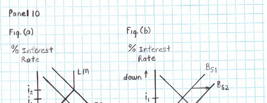
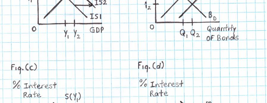
26 rises and national income increases. One of the reasons a business cycle expansion is likely to occur is because of an increase in investment spending. The more investors expect to profit from business opportunities, the more they will increase their investment spending regardless of the interest rate. This will cause the IS curve to shift to the right. Panel 10 presents the relevant markets which are affected by a change in investment. Fig. (a) shows the IS-LM market. The IS-LM market is a summary of the other markets presented in the panel and shows the end result of an increase in investment on the economy's income and interest rate. Here the shift in the IS curve from IS1 to IS2 causes an increase in both income and the interest rate. It is assumed in this example that savers are holding speculative balances because the LM curve slopes upward and is not vertical. Fig. (b) is the bond market and this is actually the starting point of the business cycle expansion. This is where investors increase their supply of bonds from Bs1 to Bs2. When investors increase the amount of their outstanding debt in order to finance their investments the interest rate rises. Remember that only in the bond market does the interest rate on the vertical axis rise as we go down the axis. Fig. (c) shows the increase in investment in market for loanable funds. Note that the interest rate in this market goes up to i3. This is because we are still at the income level of Y1, the investment spending has yet to increase income. So far we have only shown how the exchange of bonds and funds between savers and investors affect the interest rate. Fig. (d) shows the market for balances. The increase in investment causes the Mt curve to shift form Mt1 to Mt2. Because of the higher interest rate, savers are willing to give up some of their speculative balances and buy bonds. The quantity of transaction balances increase. Fig. (e) shows the market for money. Because the shift in the supply of bonds caused the interest rate to go up, the interest rate in the market for money is now at i2 (point A) and the market for money is in disequilibrium for now because the interest rate is higher than the equilibrium level for that market. Now we arrive at the affect of the increase in investment on the level of income. Fig. (f) shows the income-expenditure model. The increase in investment causes the aggregate demand curve to shift upward and the increase in aggregate demand changes income to a higher level from Y1 to Y2. Fig. (g) shows the income effect on the market for money. A higher level of income causes the demand for money to increase and the demand curve to shift upward. When the demand curve shifts upward, the interest rate rises from i1 to i2. The theory of asset demand tells us that when income is rising during a business cycle expansion, the demand for money will rise. People will want to hold more money as a store of wealth and people will want to

27 carry out more transactions using money. It is important to note here that transaction balances must be acquired by investors before the increase in income; the shift in the demand for money is shown after the increase in income, because the increase in income is what actually increases the amount of transactions. Fig. (h) shows the income effect on the market for loanable funds. The increase in income shifts the savings curve from S1 to S2 and the increase in savings reduces the interest rate from i3 to i2. Now all markets are in equilibrium with the interest rate at i2 and the income level at Y2. Again, this is summarized by the IS-LM market in fig. (a). As long as the economy remains in equilibrium, the flow of bonds supplied and demanded each period will be the same and the interest rate will remain at i2, as seen in fig. (b). Monetary policy is the control of the interest rate and money supply by the Fed. In the short run the quantity of money affects the economy through changes in the interest rate. Monetary policy influences the interest rate which in turn affects the level of planned investment. In this example we will assume that savers do not want to hold speculative balances, so the LM curve will be vertical. The monetary transmission mechanism is the process by which changes in the quantity of money influences the level of income. A simple transmission mechanism can be expressed as: M^>iv>I^>AD^>Y^. Where an increase (^) in the quantity of money (M), reduces (v) the interest rate (i), the lower interest rate stimulates (^) investment spending (I), which leads to an increase (^) in aggregate demand (AD). The increase in aggregate demand causes income (Y) to rise (^). Suppose the Fed believes that the economy is operating below its potential and decides to stimulate output and employment by increasing the money supply.

28

29

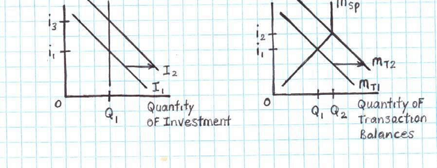
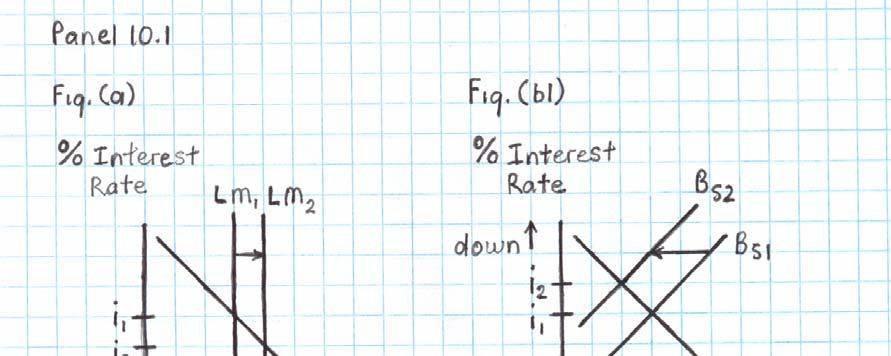
30 Panel 10.1 presents the relevant markets which are affected by the Fed's increase in the money supply. Fig. (a) shows the IS-LM market. The IS-LM market is a summary of the other markets presented in the panel and shows the end result of an increase in the money supply on the economy. Here the shift in the LM curve from LM1 to LM2 causes an increase in

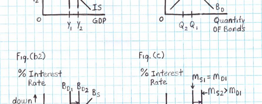
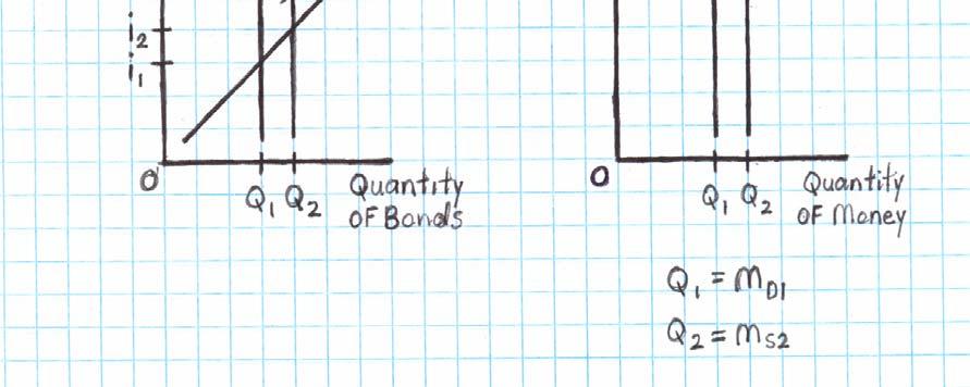
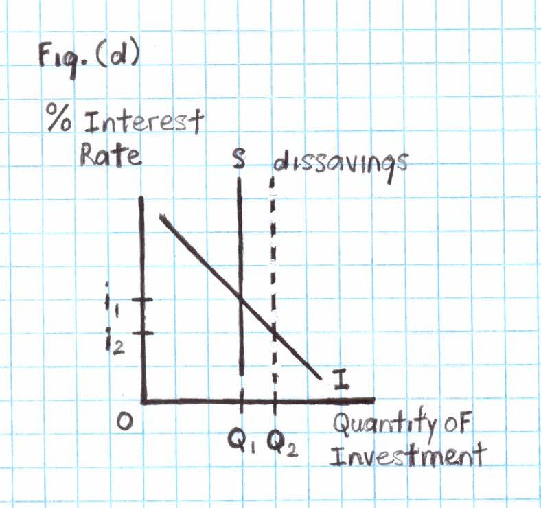
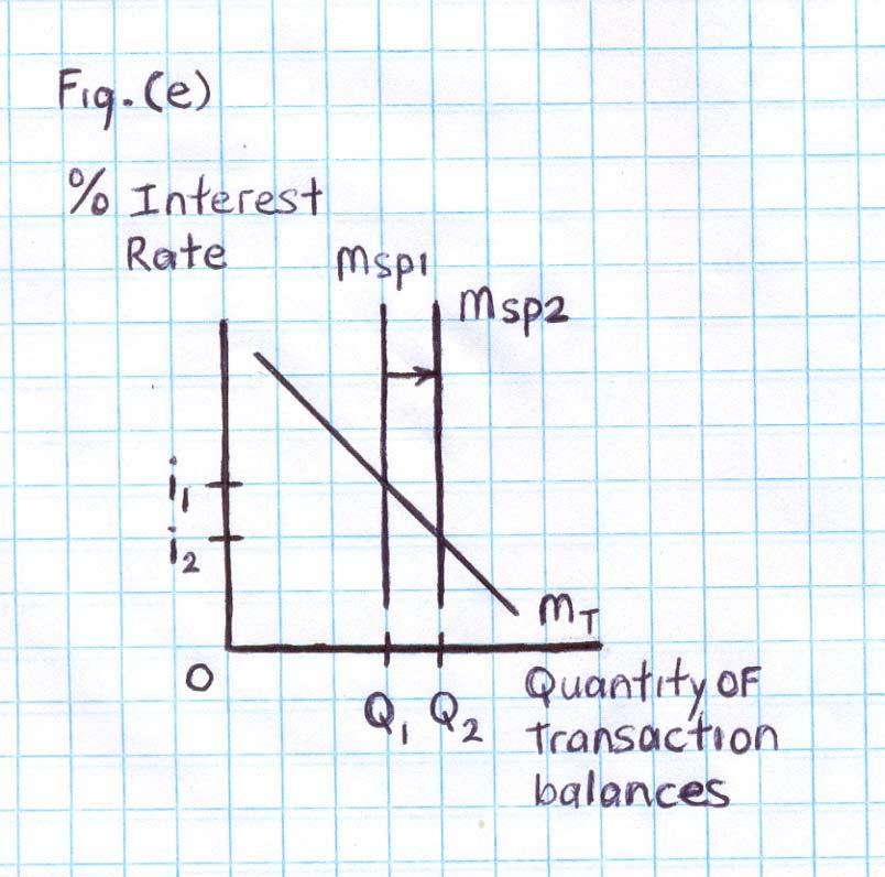
31 income and a fall in the interest rate. Fig. (b) shows the bond markets involved and this again is the actual starting point of the monetary expansion. Fig. (b1) is the bond market of stocks between the Fed and savers, fig. (b2) is the bond market of flows between savers and investors. The action in these bond markets are virtually the same as the analysis of a Fed injection in section 8.2. When the Fed buys bonds from savers, the bond supply curve shifts to the left from Bs1 to Bs2. This reduces the quantity of bonds and increases the money supply. This action has a simultaneous affect in the market for money in fig. (c). In the market for money the increase of the money supply is indicated by a rightward shift of the money supply curve from Ms1 to Ms2. Notice here that the money supply is greater than money demand. The increase of the money supply increases savers speculative balances. Consequently, savers are holding more of their wealth as money in speculative balances than they would prefer at interest rate i1. So they try to exchange their excess balances of money for bonds. This shifts the bond demand curve to the right in fig. (b2), from Bd1 to Bd2. This causes the interest rate to fall from i1 to i2. This increase in the demand for bonds is a process called dissavings which is shown in fig. (d) of the loanable funds market by the dotted line. This market shows the increase in investment due to a lower interest rate. Notice that this market is now in disequilibrium because investment is greater than savings. In fig. (e), savers supply their excess balances to investors in the market for balances. The Msp curve shifts to the right and lowers the interest rate. The increase in investment leads to an upward shift in the aggregate demand curve and raises income from Y1 to Y2 in Fig. (f). Fig. (g) shows the affect of the higher level of income on the demand for money. The increase in income causes the money demand curve to shift from Md1 to Md2 and now the market for money is in equilibrium because the money supply equals money demand. When savers got rid of their excess balances, investors used that money to increase income, which also increased transactions, until the excess balances were eliminated. Fig. (h). Shows the income effect on the loanable funds market. The increase in income caused the savings curve to shift form S1 to S2 and the interest rate to fall to i2. Now all markets are in equilibrium with the interest rate at i2 and the income level at Y2. Again, this is summarized by the IS-LM market in fig. (a). As long as the economy remains in equilibrium the interest rate will settle and there will be no tendency for it to move any further. It is important to note here that the LM cure, the money demand curve, and the bond demand curve were all vertical because of our assumption that savers do not hold speculative balances. If they did, those curves would have been downward sloping for the bond and

32 money demand curves and upward sloping for the LM curve. It is also important to note that, if savers had decided to hold the entire amount of the increase in the money supply as speculative balances, the Fed's monetary injection would have failed to increase income and employment. So for a quick summary of the Fed's monetary expansion, with fixed prices an injection may do nothing depending on savers demand for speculative balances, or it may have a direct affect on output by increasing output. With flexible prices, a monetary injection may just increase prices with no affect on output, or it may affect both prices and output having an increase in both. Now suppose that an increase in investment and an increase in the money supply occur simultaneously. A rise in investment that does not depend on the interest rate will shift the investment demand curve to the right in the loanable funds market. This increase in investment causes the IS curve in fig to shift to the right from IS1 to IS2. An increase in the money supply will shift the money supply curve in the market for money to the right. In the IS-LM market, it moves the LM curve to the right as shown in fig from LM1 to LM2. The increase in investment causes a shift upward in the aggregate demand curve which raises income. The final result is that both the IS and LM curves shift and increase the equilibrium level of income but does not change the interest rate. An increase in investment spending with no change in the money supply raises the interest rate. The rise in the interest rate dampens the increase in income. If the money supply

33 increases by just the amount necessary to prevent the rise in the interest rate, the full expansionary effect of the increase in investment on income will be realized. Without a rise in the interest rate, the increase in income is larger, and this is what we find in fig If the appropriate monetary policy is pursued to prevent a rise in the interest rate, the increase in income will be larger than if no policy action were taken. Now let's examine an autonomous increase in income. Imagine an application of a new technology that causes an autonomous increase in output by making the production process more efficient. An increase in income without a corresponding increase in expenditure will cause disequilibrium. When income is greater than expenditure, market forces will move the economy toward equilibrium. This means that income must decrease until it matches expenditure erasing the gains from the new technology and increase in income. The market forces that decrease income, stems from the fact that an increase in income is an increase in required transaction balances. Since the supply of transaction balances do no increase, income and transaction demand must decrease to where they equal the supply of transaction balances. For the increase in income to be sustained, there must be a matching increase in expenditure. Either the investors or the Fed or both must pay for the increase in income. If investors increase their expenditure, they must increase their supply of bonds (a shift in the bond supply curve to the right causing the interest rate to rise and drawing down savers speculative balances). This will cause the IS curve to shift to the right. When the Fed pays for the increase in income, the process of dissavings will cause the demand for bonds curve to shift to the right reducing the interest rate. This will allow the supply of transaction balance to increase to equal the required transaction demand. This will shift the LM curve to the right. If both the Fed and investors both pay for the increase in output, both the IS and LM curves will shift. The interest rate will remain unchanged, and only income will increase. If the Fed does nothing, the quantity of money in the economy remains unchanged and the interest rate rises because of the greater demand for transaction balances. Alternatively, the Fed can try to keep the interest rate at or below its initial level by increasing the supply of money. Which policy the Fed chooses to implement will depend on the Fed's target for the interest rate. If the economy is growing to fast, a higher interest rate will help slow the economy down. If the economy is growing to slow, a lower interest rate may help speed up the growth in income.

34 Finally, let's examine an autonomous demand for money. Panel 10.3, shows the IS-LM market and the market for balances. Fig. (a) shows the result of an autonomous demand for money in the IS-LM market. An autonomous demand for money raises the interest rate and decreases income indicated by the leftward shift in the LM curve. In order for the economy to remain at interest rate i1, savers must devote all of their savings to bonds. If savers devote a portion of their savings to speculative balances, these speculative balances must come out of transaction balances. A reduction in the quantity of transaction balances will decrease the level of income. The market for balances is indicated by fig. (b). An increase in the demand for speculative balances will decrease the supply of speculative balances in the market for balances and will also increase the interest rate. The shift of the Msp curve to the left decreases transaction balances. Panel 8.6, shows the corresponding actions in the bond and loanable funds markets. Savers can devote their savings to bonds each period and increase their assets of bonds, but savers cannot devote their savings to speculative balances each period and increase their assets of speculative balances without causing a decrease in the income level. This is because savers or investors cannot increase the money supply, but investors can and do increase the quantity of bonds each period. The money supply is controlled by the Fed. So, when investors demand transaction balances, this must reduce speculative balances. And when savers demand speculative balances, this must reduce transaction balances. This becomes apparent when examining fig. 6. So, if savers want