slides chapter 9 nominal rigidity exchange rates, and unemployment

Transcription

1 slides chapter 9 nominal rigidity exchange rates, and unemployment Princeton University Press, 2017

2 Contents 9.1 An Open Economy With Downward Nominal Wage Rigidity 9.2 Currency Pegs 9.3 Optimal Exchange Rate Policy 9.4 Empirical Evidence On Downward Nominal Wage Rigidity 9.5 The Case of Equal Intra- And Intertemporal Elasticities of Substitution 9.6 Approximating Equilibrium Dynamics 9.7 Parameterization of the Model 9.8 External Crises and Exchange-Rate Policy: A Quantitative Analysis 9.9 Empirical Evidence On The Expansionary Effects of Devaluations 9.10 The Welfare Costs of Currency Pegs 9.11 Symmetric Wage Rigidity 9.12 The Mussa Puzzle 9.13 Endogenous Labor Supply 9.14 Production in the Traded Sector 9.15 Product Price Rigidity 9.16 Staggered Price Setting: The Calvo Model 1

3 Roadmap Chapter 9 develops a theoretical framework in which nominal rigidities result in inefficient adjustments to aggregate disturbances framework can be used in an intuitive graphical manner to demonstrate how nominal rigidities amplify the business cycle in open economies but framework can also be used to derive quantitative predictions useful for policy evaluation 2

4 Some Motivation: Peripheral Europe and the Global Crisis of 2008 Take a look at the next slide. The inception of the Euro in 1999 was followed by massive capital inflows into the region, possibly driven by expectations of quick convergence of peripheral and core Europe. Large current account deficits and large increases in nominal hourly wages, with declining rates of unemployment between 2000 and When the global crisis of 2008 starts, capital inflows dry up abruptly. Peripheral Europe suffers a severe sudden stop (sharp reductions in current account deficits). In spite of the collapse in aggregate demand and the lack of a devaluation, nominal hourly wages remain as high as at the peak of the boom. Massive unemployment affects all countries in the region. 3

5 Figure 9.1 Boom-Bust Cycle in Peripheral Europe: Current Account / GDP 110 Labor Cost Index, Nominal 14 Unemployment Rate Percent Index, 2008 = Percent Date Date Date Data Source: Eurostat. Labor Cost Index, Nominal, is the nominal hourly wage rate in manufacturing, construction and services (including the public sector, but for Spain.) Data represents arithmetic mean of Bulgaria, Cyprus, Estonia, Greece, Ireland, Lithuania, Latvia, Portugal, Spain, Slovenia, and Slovakia. 4

6 Percent Current Account / GDP: Cyprus Index, 2008 = 100 Nominal Hourly Wages: Cyprus Percent Unemployment Rate: Cyprus Percent Percent Percent Current Account / GDP: Greece Index, 2008 = 100 Current Account / GDP: Ireland Index, 2008 = 100 Current Account / GDP: Portugal Index, 2008 = 100 Nominal Hourly Wages: Greece Nominal Hourly Wages: Ireland Nominal Hourly Wages: Portugal Percent Percent Percent Unemployment Rate: Greece Unemployment Rate: Ireland Unemployment Rate: Portugal The Disaggregated Story: Boom- Bust Cycles in Cyprus, Greece, Ireland, Portugal, and Spain. Percent 10 Current Account / GDP: Spain Index, 2008 = 100 Nominal Hourly Wages: Spain Percent Unemployment Rate: Spain

7 The previous two figures suggest the following narrative: Countries in the periphery of the European Union, such as Ireland, Portugal, Greece, and a number of small eastern European countries adopted a fixed exchange rate regime by joining the Euroarea. Most of these countries experienced an initial transition into the Euro characterized by low inflation, low interest rates, and economic expansion. However, history has shown time and again that fixed exchange rate arrangements are easy to adopt but difficult to maintain. (Example: Argentina s 1991 convertibility plan.) The Achilles heel of currency pegs is that they hinder the efficient adjustment of the economy to negative external shocks, such as drops in the terms of trade or hikes in the interest-rate. Such shocks produce a contraction in aggregate demand that requires a decrease in the relative price of nontradables, that is, a real depreciation of the domestic currency, in order to bring about an expenditure switch away from tradables and toward nontradables. In turn, the required real depreciation may come about via a nominal devaluation of the domestic currency or via a fall in nominal prices or both. The currency peg rules out a devaluation. Thus, the only way the necessary real depreciation can occur is through a decline in the nominal price of nontradables. However, when nominal wages are downwardly rigid, producers of nontradables are reluctant to lower prices, for doing so might render their enterprises no longer profitable. As a result, the necessary real depreciation takes place too slowly, causing recession and unemployment along the way. This narrative goes back at least to Keynes (1925) who argued that Britain s 1925 decision to return to the gold standard at the 1913 parity despite the significant increase in the aggregate price level that took place during World War I would force deflation in nominal wages with deleterious consequences for unemployment and economic activity. Similarly, Friedman s (1953) seminal essay points at downward nominal wage rigidity as the central argument against fixed exchange rates. 6

8 To formalize this narrative let s build an open economy model with downward nominal wage rigidity a traded and a nontraded sector involuntary unemployment To produce quantitative predictions Estimate the key parameters of the model (with particular attention on the parameter governing downward wage rigidity) and estimate the driving forces. Characterize response to large negative external shock under a peg and show that the model can explain the observed sudden stop. Characterize optimal exchange rate policy. Quantify the costs of currency pegs in terms of unemployment and welfare. The material is based on Schmitt-Grohé and Uribe (JPE, 2016). 7

9 9.1 An Open Economy with Downward Nominal Wage Rigidity (The DNWR Model) 8

10 Downward Nominal Wage Rigidity (DNWR) W t γ W t 1 (9.6) W t = nominal wage rate in period t γ = degree of downward wage rigidity. γ = 0 fully flexible wages. Think of γ as being around 1. The empirical evidence presented later in this chapter suggests γ = 0.99 at quarterly frequency. 9

11 Traded and Nontraded Goods Stochastic endowment of tradable goods: yt T. Stochastic country interest rate: r t. Nontraded goods, yt N, produced with labor, h t: yt N = F(h t ). Law of one price holds for tradables: Pt T = E t Pt. Pt T, nominal price of tradable goods. E t, nominal exchange rate, domestic-currency price of one unit of foreign currency (E t depreciation of domestic currency). Pt, foreign currency price of tradable goods. Assume that Pt = 1, so that P t T = E t Section 9.14 relaxes this assumption. 10

12 The Nontraded Sector Profits, Φ t : Φ t = P N t F(h t) W t h t P N t, nominal price of nontradables. Firms maximize profits taking as given Pt N Condition: and W t. Optimality Divide by P T t = E t and rearrange p t P N t P T t P N t F (h t ) = W t p t = W t/e t F (h t ), relative price of nontradables in terms of tradables. Interpret this optimality conditions as a supply schedule for nontradables, see next slide. 11

13 The Supply Schedule of Nontradables Let s derive the supply schedule for nontradables in the space (y N, p) given the real wage, W t /E t. Note that real marginal cost of one unit of nontraded good Use h = F 1 (y N ) to obtain marginal cost = W t/e t F (h t ) marginal cost = W t /E t F (F 1 (y N ) By the profit maximization condition marginal cost equals price or p t = W t /E t F (F 1 (y N t )) Interpret this relation as a supply schedule of nontradables given the real wage. 12

14 Figure 9.3 The Supply Of Nontradables Supply schedule: p t = W t/e t F (F 1 (y N t )) Price, p W 1 /E 0 F (F 1 (y N )) Properties: upward sloping, the higher the price, the more a firm wishes to produce, given factor prices. W 0 /E 0 F (F 1 (y N )) A decrease in nominal wage from W 1 to W 0 < W 1 shifts the supply schedule down and to the right. A devaluation E t (not shown) shifts the supply schedule in the same manner as a nominal wage cut. Quantity, y N 13

15 Households subject to max {c T t,cn t, d t+1} E 0 β t U(c t ) (9.1) t=0 c t = A(c T t, c N t ) (9.2) P T t c T t + P N t c N t + E t d t = P T t y T t + W t h t + E t d t r t + Φ t (9.3) h t h (9.7) First constraint: Consumption is a composite of traded and nontraded goods. A(.,.) increasing, concave, and HD1. Second constraint: d t = one-period debt chosen in t, due in t+1. Debt is denominated in units of foreign currency full liability dollarization. Original Sin: In emerging countries almost 100% of external debt issued in foreign currency (Eichengreen, Hausmann, and Panizza, 2005). Country interest rate, r t, is stochastic. Third constraint: Workers supply h hours inelastically, but may not be able to sell them all. They take h t h as given. Section 9.13 relaxes this assumption. 14

16 Optimality Conditions Associated with the Household Problem A 2 (c T t, cn t ) A 1 (c T t, cn t ) = p t (9.5) λ t = U (A(c T t, cn t ))A 1(c T t, cn t ) λ t = β(1 + r t )E t λ t+1 P T t ct t + P N t cn t + E t d t = P T t yt t + W th t + E t d t r t + Φ t h t h 15

17 The Demand For Nontradables Look again at the optimality condition (9.15) A 2 (c T t, cn t ) A 1 (c T t, cn t ) = p t. (9.15) If A(c T, c N ) is concave and HD1, then given c T t, the left-hand side is decreasing in c N t. This means that, all other things equal, an increase in p t reduces the desired demand for nontradables, giving rise to the downward sloping demand schedule shown in the next slide. Note that c T t acts as a shifter of the demand schedule for nontradables: given p t, an increase in c T t is associated with an equiproportional desired increase in c N t. Of course, this shifter is endogenously determined. 16

18 Figure 9.2 The Demand For Nontradables p t = A 2(c T t, cn t ) A 1 (c T t, cn t ) (9.15) Price, p A 2(c T 1,cN ) A 1(c T 1,cN ) A 2(c T 0,cN ) A 1(c T 0,cN ) here we treat c T t as a shifter of the demand schedule. An increase in c T t from c T 0 to c T 1 > c T 0, shifts the demand schedule up and to the right. Quantity, c N 17

19 Closing of the Labor Market Nominal wages are downwardly rigid Labor demand may not exceed supply Impose the following slackness condition: W t γw t 1 (9.6) h t h (9.7) ( h h t ) ( W t γw t 1 ) = 0 (9.8) This slackness condition says that, if there is involuntary unemployment (h t < h), then the lower bound on nominal wages must be binding. It also says that if the lower bound on nominal wages is not binding ( W t > γw t 1 ), then the labor market must feature full employment. Market clearing in the Nontraded Sector c N t = y N t = F(h t ) 18

20 A competitive equilibrium is a set of stochastic processes {c T t, h t, w t, d t+1, p t, λ t } t=0 satisfying c T t + d t = y T t + d t r t (9.9) λ t = U (A(c T t, F(h t )))A 1 (c T t, F(h t )) (9.13) λ t 1 + r t = βe t λ t+1 (9.14) p t = A 2(c T t, F(h t)) A 1 (c T t, F(h t)) (9.15) p t = w t F (h t ) (9.16) w t γ w t 1 ɛ t (9.17) h t h (9.18) ( ( h h t ) w t γ w ) t 1 = 0 ɛ t (9.19) given an exchange rate policy {ɛ t } t=0, initial conditions w 1 and d 0, and exogenous stochastic processes {r t, yt T } t=0. To characterize the eqm we must specify the exchange-rate regime. We will turn to this next. 19

21 A Graphical Representation of (Partial) Equilibrium Why partial, because for the moment we take c T as given. In equilibrium, c N = y N = F(h). This means that we can draw Figures 9.2 and 9.3 in the employment-relative price of nontradables space, that is, in the space (h,p) The Demand for Nontradables Price, p Price, p The Supply of Nontradables W 0 /E 0 F (h) A 2(c T 0,F(h)) A 1(c T 0,F(h)) Employment, h Employment, h 20

22 In eqm both (9.15) and (9.16) must hold. We refer to the value of h at which these schedules intersect for given W 0 /E 0 and c T 0 as labor demand, and denote it h d Price, p W 0 /E 0 F (h) p A 2(c T 0,F(h)) A 1(c T 0,F(h)) h d Employment, h Next add the labor supply schedule to the graph. Two generic cases emerge: at given real wages, labor demand exceeds labor supply, or labor supply exceeds labor demand. Let s consider the first case first. 21

23 Suppose given W 0 /E 0, labor demand exceeds labor supply: Price, p W 0/E 0 F (h) real wage rises to clear the labor market, W 0, until h d = h s. Price, p W 1 /E 0 F (h) W 0 /E 0 F (h) A 2(c T,F(h)) A 1(c T,F(h)) B A 2(c T,F(h)) A 1 (c T,F(h)) C B h s h d Employment, h In eqm, there is full employment, h t = h h s h d Employment, h 22

24 Now suppose given W 0 /E 0, labor supply exceeds labor demand: Price, p A 2(c T 0,F(h)) A 1(c T 0,F(h)) D W 1/E 0 F (h) to clear the labor market the real wage must fall, but nominal wages cannot fall due to DNWR (assume γ = 1). Thus, unless the monetary authority devalues, E, the labor market will fail to clear. h d h s Employment, h In eqm, absent a devaluation there is unemployment, h t < h In the following sections, we will use the graphical framework (as well as quantitative methods) to analyze boom and bust cycles. 23

25 9.2 Currency Pegs 24

26 The exchange rate policy is a peg E t = E 0 ; t 0. Use the graphical apparatus just developed to show that a boombust cycle leads as documented in Figure 9.1 to nominal wage growth and real appreciation during the boom phase involuntary unemployment and insufficient real depreciation during the bust phase 25

27 Figure 9.4 Adjustment to a Boom-Bust Cycle under a Currency Peg p A 2(c T 1,F(h) ) A 1(c T 1,F(h) ) W 1 /E 0 F (h) p boom A 2(c T 0,F(h) ) A 1(c T 0,F(h) ) C p bust D B W 0 /E 0 F (h) = W 1/E 1 F (h) p 0 A h bust h h c T 1 < ct 0 negative external shock possibly caused by r t 26

28 Observations on Figure 9.4: Adjustment in a Boom-Bust Episode The initial situation is point A. At point A there is full employment, h = h. Now a boom starts. We capture this by an increase in c T (perhaps because r falls). Given nominal wages the economy moves to point B. But at point B, there is excess demand for labor. Thus nominal wages will rise. By how much? Until the excess demand for labor has disappeared. That will be at point C. Thus the boom leads to an increase in nominal wages (W ) and a real appreciation (p ). The economy continues to operate at full employment. Next the boom is over and the bust comes. We capture this by assuming that c T falls back to its original level, c T 0. This shifts the demand for nontradables back to its original position. The new intersection between supply and demand is at point D. At D, labor supply exceeds labor demand. However, because nominal wages are downwardly rigid and the nominal exchange rate is fixed, the supply schedule does not shift, (for simplicity, in the figure, we assume γ = 1). Thus the economy is stuck at point D. At point D, there is involuntary unemployment ( h h bust ) and there is insufficient real depreciation, i.e., p t does not fall enough (that is, does not fall to p 0 ) to restore full employment. 27

29 The Link between Volatility and Average Unemployment The present model predicts that aggregate volatility increases the mean level of unemployment. This prediction gives rise to large welfare benefits of stabilization policy. This prediction is not due to the assumption of downward nominal wage rigidity, but due to the assumption that employment is determined by the minimum of labor demand and labor supply. (Note: key difference with Calvo-style sticky wage models in which employment is always demand determined.) Downward nominal wage rigidity amplifies the connection between aggregate volatility and mean unemployment. 28

30 To see this consider the following example: U(A(c T t, cn t )) = ln ct t + ln cn t d t = 0 (no access to international financial markets) c T t = yt t. y T t = { 1 + σ prob σ prob 1 2 E(y T t ) = 1 and var(yt t ) = σ2. F(h t ) = h α t h = 1 E t = E (currency peg) W 1 = αe 29

31 The equilibrium conditions associated with this economy are (we list all except wage adjustment, for which we will consider two cases): c T t c N t = p t αp t (h t ) α 1 = W t /E c T t = y T t c N t = h α t Step 1: Find labor demand: h d t = αyt t W t /E Step 2: Find equilibrium labor as h t = min{ h, h d t } 30

32 Case 1: Assume bi-directional nominal wage rigidity. W t = αe Then, h d t = yt t, and the equilibrium level of employment is h t = { 1 σ if y T t = 1 σ 1 if y T t = 1 + σ Let u t h h t denote the unemployment rate. It follows that the equilibrium distribution of u t is given by { σ with probability 1 u t = 2 0 with probability 1. 2 The unconditional mean of the unemployment rate is then given by E(u t ) = σ 2. Average level of unemployment increases linearly with the volatility of tradable endowment, in spite of the fact that wage rigidity is symmetric! 31

33 Case 2: assume only downward nominal wage rigidity, W t W t 1 Then, W t = α(1 + σ) > α and { 1 σ h t = 1+σ if yt T = 1 σ 1 if yt T = 1 + σ E(u t ) = σ/(1 + σ) > σ/2 (recall that σ must be less than 1). Thus uni-directional wage rigidity exacerbates the link between mean unemployment and volatility. 32

34 The Peg-Induced Externality Under a currency peg and downward nominal wage rigidity, a good shock, in this example that follows a fall in the country interest rate r t, can be the prelude to bad things to happen later. The reason is that individual agents do not internalize that during the boom nominal wages increase too much, putting the economy in a vulnerable position once the good shock fades away. Consider the following environment: U(A(c T t, cn t )) = ln ct t + ln cn t F(h t ) = h α t ; 0 < α < 1 h = 1; yt T = y T > 0; γ = 1; β(1+r) = 1; d 0 = 0; w 1 = αy T r t = { r t > 0 r < r t = 0 33

35 The Peg-Induced Externality (Continued) In a couple of slides, you ll find the solution of the equilibrium in algebraic and graphical form. To help the interpretation of those slides, it is of use to discuss intuitively what is going on in this economy: The fall in the interest rate in period 0 induces an expansion in the desired demand for consumption goods, of all types, tradables and nontradable. The increased demand for tradables causes a trade balance deficit, a deficit in the current account, and an increase in external debt in period 0. The increased demand for nontradables cause a rise in wages and a rise in the relative price of nontradables (i.e., an appreciation of the real exchange rate). 34

36 The Peg-Induced Externality (Continued) In period 1, the interest rate goes back up to its permanent value r, causing a contraction in the demand for consumption goods (both tradables and nontradables), and a reversal in the trade balance and the current account. The contraction in the demand for nontradables causes a derived contraction in the demand for labor. However, because nominal wages are downwardly rigid and the nominal exchange rate is fixed, the real wage fails to fall, causing involuntary unemployment. Involuntary unemployment is highly persistent. (In fact, in this example, because γ = 1, it never disappears.) 35

37 The Peg-Induced Externality (Continued) The equilibrium has the following closed-form solution: [ c T 0 = 1 yt 1 + r + r ] > y T 1 + r [ c T t = y T r + r 1 + r 1 + r1 + r [ d t = y T r 1 + r h 0 = 1; ] ] > 0, h 1 = h 2 = 1 + r 1 + r < 1 < y T, The following slide displays the same information graphically. 36

38 Figure 9.5 A Temporary Decline in the Country Interest Rate Country Interest Rate, r t Consumption of Tradables, c T t r r Time, t Debt, d t y T Time, t Unemployment, ( h h)/ h Time, t Real Wage, w t Time, t Real Exchange Rate, Pt N /Pt T αy T Time, t Time, t currency peg flexible wage economy or optimal exchange rate economy 37

39 Section 9.3 Optimal Exchange Rate Policy 38

40 Motivation We have just seen that under an exchange rate peg a negative external shock may lead to involuntary unemployment. How would optimal exchange rate policy look like? In this section we show that under optimal policy there is (1) full employment and (2) negative external shocks call for devaluations. We begin with a graphical explanation. 39

41 The graph on the next slide illustrates how the optimal exchange rate policy works The initial situation is point A. Suppose a negative shock (possibly an increase in the country interest rate), shifts the demand schedule down and to the left. Without government intervention, the supply schedule does not move, because W is downwardly rigid. The equilibrium would then be point B, with involuntary unemployment equal to h h PEG. Suppose now that the government devalues the domestic currency from E 0 to E 1 > E 0. The devaluation lowers the real wage from W 0 /E 0 to W 0 /E 1, causing the supply schedule to shift down and to the right. If the devaluation is just right, the new supply schedule will cross the new demand schedule at point C, preserving full employment (we say preserving and not restoring full employment because the economy jumps from A to C, without visiting B). Note: the fall in labor cost caused by the drop in the real wage allows firms to cut prices from p 0 to p OPT and induces households to switch expenditure away from tradables and toward nontradables. Take another look at the graph for the analytical example in of a temporary fall in r 0. The broken lines display the equilibrium under optimal exchange-rate policy. 40

42 Optimal Exchange-Rate Policy (again, assume γ = 1) p A 2(c T 0,F(h) ) A 1(c T 0,F(h) ) p 0 p PEG A 2(c T 1,F(h) ) A 1(c T 1,F(h) ) B A W 0 /E 0 F (h) p OPT C W 0 /E 1 F (h) h PEG h h c T 1 < ct 0 (negative shock, possibly r t ) E 1 > E 0 (optimal devaluation) 41

43 The Ramsey Optimal Exchange-Rate Policy The Ramsey government solves the problem: max E 0 β t U(A(c T t, F(h t ))) t=0 subject to (9.9) and (9.13)-(9.19). Strategy: solve a less constrained problem and then show that its solution satisfies (9.9) and (9.13)-(9.19). 42

44 Consider the less restricted problem of choosing {c T t, h t, d t+1 } t=0 to max E 0 t=0 β t U(A(c T t, F(h t))) subject to the following subsect of the equilibrium coditions: c T t + d t = y T t + d t r t (9.9) h t h (9.18) Clearly, the solution for labor is h t = h for all t or full employment at all times. Intuition: One nominal friction and one instrument that can fully offset it. Hence possible to obtain the flexible wage allocation (which here coincides with the first best). But to show that this is indeed the allocation under the optimal exchangerate policy, we must show that the solution to the above social planner s problem satisfies the all of the competitive equilibrium conditions, that is, conditions (9.9) and (9.13)-(9.19). To see this, proceed by construction: set λ t to satisfy (9.13), p t to satisfy (9.15), w t to satisfy (9.16), ɛ t to satisfy (9.17), (9.18) is a constraint of the social planner s problem, and so is (9.9). Because h t = h, (9.19) holds. That (9.14) holds follows from the definition of λ t and the first-order condition of the social planner. 43

45 An important reference point: The full-employment real wage, denoted ω(c T t ), defined as the real wage that clears the labor market, ω(c T t ) A 2(c T t, F( h)) A 1 (c T t, F( h)) F ( h); ω (c T t ) > 0 Set the (gross) devaluation rate, ɛ t = E t /E t 1, to eliminate unemployment: ɛ t γw t 1/E t 1 ω(c T t ) Note: There is a whole family of optimal exchange-rate policies. Under any member of this policy, h t = h and w t = ω(c T t ) for all t. 44

46 When is it inevitable to devalue? Optimal exchange rate policy is: ɛ t γw t 1/E t 1 ω(c T t ) Because ω (c T t ) > 0, optimal devaluations occur in periods of contraction of aggregate demand. It follows that contractions are devaluatory as opposed to devaluations being contractionary. 45

47 Under optimal exchange rate policy external debt and tradable consumption are determined by the solution to v OPT (yt T, r { t, d t ) = max U(A(c T t, F( h)) + βe t v OPT (y T {d t+1,c T t } t+1, r t+1, d t+1 ) } subject to y T t + d t r t = d t + c T t 46

48 9.4 Empirical Evidence On Downward Nominal Wage Rigidity 47

49 Downward nominal wage rigidity is the central friction in the present model natural to ask if it is empirically relevant. Downward nominal wage rigidity has been studied empirically from a number of perspectives: Evidence from micro and macro data. Studies focusing on rich, emerging, and poor countries. Studies focusing on formal and informal labor markets. By product: Will obtain an estimate of the parameter γ governing wage stickiness in the model (useful for quantitative analysis). 48

50 Downward Nominal Wage Rigidity A.) Evidence From Micro Data from Developed Countries 1. United States, , SIPP panel data 2. United States, , SIPP panel data 3. United States, , CPS panel data 4. Other Developed Countries 49

51 1.) United States, , SIPP panel data Probability of Decline, Increase, or No Change in Wages Interviews One Year apart Males Females Decline 5.1% 4.3% Constant 53.7% 49.2% Increase 41.2% 46.5% Source: Gottschalk (2005). Note: Male and female hourly workers not in school, 18 to 55 at some point during the panel. All nominal-wage changes are within-job wage changes, defined as changes while working for the same employer. SIPP panel data. Large mass at Constant suggests nominal wage rigidity. Small mass at Decline suggests downward nominal wage rigidity. 50

52 2.) United States , SIPP panel data Distribution of Non-Zero Nominal Wage Changes Source: Barattieri, Basu, and Gottschalk (2012). SIPP panel data. 51

53 3.a) United States 2011, CPS data. Distribution of Nominal Wage Changes, U.S Source: Daly, Hobijn, and Lucking (2012). 51

54 3.b) The next slide shows the distributions of Nominal Wage Changes in the United States for each year from 1997 to 2016, from CPS panel data Nominal wage change: Year-over-year log changes in nominal hourly wages of hourly-paid job stayers. In each panel, the horizontal axis shows bins of year-over-year percent change in the nominal hourly wage of an hourly-paid jobstayer. The bin size is two percent, with the exception of a wage-freeze bin, which is defined as an exact zero change. The vertical axis measures the share of workers in each bin. Each wage change distribution is based on about 5,000 workers. 52

55 Source: Jo, Schmitt-Grohé, and Uribe (2017). 53

56 Observations on the figure Large spike at zero wage changes. Many more wage increases than wage cuts. Fraction of wage freezes is cyclical, rises from 15 percent in 2007 to 20 percent in Much smaller cyclical increase in wage cuts. 54

57 4.) Micro Evidence On Downward Nominal Wage Rigidity From Other Developed Countries Canada: Fortin (1996). Japan: Kuroda and Yamamoto (2003). Switzerland: Fehr and Goette (2005). Industry-Level Data: Holden and Wulfsberg (2008), 19 OECD countries from 1973 to

58 B.) Evidence From Informal Labor Markets Are nominal wages downwardly flexible in in informal labor markets, where labor unions, wage legislation, or regulation play, if any, a small role? Kaur (2012) addresses this issue by examining the behavior of nominal wages, employment, and rainfall in casual daily agricultural labor markets in rural India (500 districts from 1956 to 2008). Finds asymmetric nominal wage adjustment: W t increases in response to positive rainfall shocks W t failure to fall, labor rationing, and unemployment are observed in response to negative rain shocks. Inflation (uncorrelated with local rain shocks) tends to moderate rationing and unemployment during negative rain shocks, suggesting downward rigidity in nominal rather than real wages. 56

59 C.) Evidence From the Great Depression in the U.S. How do nominal wages behave during extraordinary contractions? The next slide shows the nominal wage rate and the consumer price index in the United States from 1923:1-1935:7. Between 1929 and 1931 the U.S. economy experienced an enormous contraction in employment of 31%. Nonetheless, during this period nominal hourly wages fell by 0.6% per year, while consumer prices fell by 6.6% per year. See the figure on the next slide. A similar pattern is observed during the second half of the Depression. By 1933, real wages were 26% higher than in 1929, in spite of a highly distressed labor market. 57

60 Figure 9.8 Nominal Wage Rate and Consumer Prices, United States 1923:1-1935: :8= log(nominal Wage Index) log(cpi Index) Year Solid line: natural logarithm of an index of manufacturing money wage rates. Broken line: logarithm of the consumer price index. 58

61 D.) Evidence From the Great Depression In Europe Countries that left the gold standard earlier recovered faster than countries that remained on gold. Left Gold Early (sterling bloc): United Kingdom, Sweden, Finland, Norway, and Denmark. Countries That Stuck To Gold (gold bloc): France, Belgium, the Netherlands, and Italy. The gold standard is akin to a currency peg. A peg not to another currency, but to gold. When the sterling-bloc left gold, they effectively devalued, as their currencies lost value against gold. The figure on the next slide shows that between 1929 and 1935 the sterling-bloc experienced less real wage growth and a larger increase in industrial production than the gold bloc. 59

62 Changes In Real Wages and Industrial Production, Finland Denmark Sweden 120 United Kingdom 110 Industrial Production, 1935, (1929=100) Norway Germany Italy Netherlands 80 Belgium France Real Wage, 1935, (1929=100) 60

63 E.) Evidence From Emerging Countries Argentina pegged the peso at a 1-to-1 rate to the dollar between 1991 and Starting in 1998, the economy was buffeted by a number of large negative shocks (weak commodity prices, large devaluation in Brazil, large increase in country premium). Not surprisingly, between 1998 and 2001, unemployment rose sharply. See the figure on the next slide. Nonetheless, nominal wages remained remarkably flat. This evidence is consistent with downward nominal wage rigidity, and suggests that γ, the parameter governing downward wage rigidity in the model, is about 1. Why γ 1? The slackness condition ( h h t )(W t γw t 1 ) (recall ɛ t = 1 between 1991 and 2001), implies that if unemployment is growing, then wages must grow at the gross rate γ. Argentine wages were flat γ 1. 61

64 4 Argentina Nominal Exchange Rate (E t ) Unemployment Rate + Underemployment Rate 40 Pesos per U.S. Dollar Percent Year Year Nominal Wage (W t ) 1.4 Real Wage (W t /E t ) 1.2 Pesos per Hour 12 Index 1996= Year Year Implied Value of γ: Around unity. 62

65 Evidence From Peripheral Europe ( ) The next slide shows the unemployment rate and nominal wage growth between 2008:Q1 and 2011:Q2 in 12 European countries that were either in the eurozone or pegging to the euro. Between 2008 and 2011, all countries in the periphery of Europe experienced increases in unemployment; Some very large increases. In spite of extreme duress in the labor market, nominal hourly wages experienced increases in most countries and modest declines in only a few. The slide following the table explains how to use the information in the table to infer a range for γ. 63

66 Table 9.2 Unemployment, Nominal Wages, and γ Evidence from the Eurozone Unemployment Rate Wage Growth Implied W 2008Q1 2011Q2 2011Q2 W 2008Q1 Value of Country (in percent) (in percent) (in percent) γ Bulgaria Cyprus Estonia Greece Ireland Italy Lithuania Latvia Portugal Spain Slovenia Slovakia Note. W is an index of nominal average hourly labor cost in manufacturing, construction, and services, including the public sector (except for Spain). Source: Schmitt-Grohé and Uribe (2016a) 64

67 How To Infer γ From European Data As explained in the analysis of the Argentine Convertibility Plan, the slackness condition of the model, (W t γw t 1 )( h h t ), implies that if unemployment increases form one period to the next, then nominal W wages must be growing at the rate γ: t W = γ. t 1 How to calculate γ: γ = ( W2011:Q2 W 2008:Q1 Subtract 0.6% per quarter to adjust for foreign inflation and long-run growth (because they are not explicitly incorporated in the model) to obtain the estimate: ) 1 13 γ [0.99, 1.022] 65

68 Quantitative Analysis (Sections and 9.10) Replication files: usg_dnwr.zip available online with the materials for this chapter. 66

69 Functional Forms Assume a CRRA form for preferences, a CES form for the aggregator of tradables and nontradables, and an isoelastic form for the production function of nontradables: U(c) = c1 σ 1 1 σ A(c T, c N ) = [ ] 1 a(c T ) 1 1 ξ + (1 a)(c N ) ξ 1 ξ F(h) = h α, with σ, ξ, a, α > 0. 67

70 The case of Equal Intra- and Intertemporal Elasticities of Substitution Consider the case Why this case is of interest: ξ = 1 σ It makes the determination of the equilibrium levels of debt, d t, and consumption of tradables, c T t, independent of the level of activity in the nontraded sector (see the next slide). As a result, the welfare consequences of exchange-rate policy or nominal wage rigidity are fully attributable to their effect on unemployment, and not on their effect on the accumulation of external debt. It facilitates the computation of equilibrium, as the equilibrium dynamics of d t and c T t can be computed separately from the equilibrium dynamics of h t, w t, c N t, and p t. As we will argue shortly, σ = 1/ξ = 2 is empirically plausible. 68

71 Debt and Tradable Consumption when ξ = 1 σ In this case, U(A(c T t, c N t )) = act t 1 σ + (1 a)c N1 σ t 1, 1 σ which is separable in c T t and c N t. Then d t and c T t solve c T t + d t = y T t + d t r t (c T t ) σ = β(1 + r t )E t (c T t+1 ) σ This subsystem is independent of h t, w t, p t, and c N t. It can be cast as a Bellman equation problem, which facilitates the quantitative analysis (more on the next slide). 69

72 Approximating Equilibrium Dynamics Under Optimal Exchange-Rate Policy when ξ = 1/σ Equilibrium processes {c T t, d t+1} solve the Bellman equation problem v OPT (yt T, r { t, d t ) = max U(A(c T t, F( h))) + βe t v OPT (y T {d t+1,c T t } t+1, r t+1, d t+1 ) } (1) subject to c T t + d t = y T t + d t r t ; and d t+1 d. (2) Approximate by value function iteration over a discretized state space (y T t, r t, d t ). Use 21 values for y T t and 11 for r t (the estimated joint process (y T t, r t) is given below). Use 501 equally spaced points for d t between 1 and Given approximated solutions to d t+1 and c T t, all other variables of the model can be backed out: h t = h, p t = A 2(c T t,f( h)) A 1 (c T t,f( h)), w t = p t F ( h), and a chosen member of the family ɛ t γw t 1 /w t. 70

73 Approximating Equilibrium Under Currency Pegs with ξ = 1/σ When ξ = 1/σ, the solution for d t+1 and c T t is as before, since it does not depend on the exchange-rate policy. for the optimal exchange-rate policy The determination of w t requires knowledge of past real wages. So, w t 1 is a relevant endogenous state. This is different from the equilibrium under optimal exchange-rate policy. Given w t 1 and c T t, the solution for w t is static (simple): First, conjecture that h t = h, and obtain w t = A 2(c T t,f( h)) A 1 (c T t,f( h)) F ( h). If w t γw t 1, this is the solution. Otherwise, w t = γw t 1, and h t solves w t = A 2(c T t,f(h t)) A 1 (c T t,f(h t)) F (h t ). Discretization of w t 1 grid: 500 points between 0.25 and 6, equally spaced in logs. 71

74 Approximating Equilibrium when ξ 1/σ Optimal Exchange-Rate Policy: As before, the solution is separable. First, the processes d t+1 and c T t solve the Bellman equation problem (1)-(2). Then, all other variables (w t, p t, c N t ) are then easily backed out. Currency Peg: The the solution is no longer separable. All equilibrium conditions must be solved jointly and becomes more complicated. Schmitt-Grohé and Uribe (JPE, 2016) develop an algorithm to handle this case. 72

75 The Driving Process: Data: Argentine data over the period 1983:Q1 2001:Q3. Exclude the period 2001:Q4 to present, because of the default episode in 2002 (no default in the model). Empirical Measure of yt T : sum of GDP in agriculture, manufacturing, fishing, forestry, and mining. Quadratically detrended. Empirical Measure of r t : Sum of Argentine EMBI+ plus 90-day Treasury-Bill rate minus a measure of U.S. expected inflation. The following slide displays the two time series. 73

76 Tradable Output and Country Interest Rate Argentina 1983:Q1 to 2001:Q3 0.2 Traded Output 70 Country Interest Rate lny T t rt in percent per year

77 Estimate the AR(1) system [ ln y T t ln 1+r t 1+r ] = A ln yt t 1 ln 1+r t 1 1+r + ɛ t, OLS Estimate of the Driving Process [ ] [ A = ; Σ ɛ = ] ; r = (3.16% per quarter). 75

78 Some Unconditional Summary Statistics Statistic y T r Std. Dev. 12% 6%yr Serial Corr Corr(yt T, r t) Mean 1 12%yr Comments: (1) High volatility of both y T t and r t ; (2) negative correlation between y T t and r t (when it rains it pours); (3) High mean country interest rate. 76

79 Calibration Parameter Value Description γ 0.99 Degree of downward nominal wage rigidity σ 2 Inverse Intertemp. elast. of subst. y T 1 Steady-state tradable output h 1 Labor endowment a 0.26 Share of tradables ξ 0.5 Intratemp. elast. of subst. α 0.75 Labor share in nontraded sector β Quarterly subjective discount factor Note: σ = 2 is widely used in business cycle analysis, and ξ = 0.5 is within the range of values estimated for emerging countries (see the survey by Akinci, 2011). Consequently, the restriction ξ = 1/σ is quite compelling on empirical and computational grounds. 77

80 Crisis Dynamics Under A Currency Peg and Under Optimal Exchange-Rate Policy We are interested in characterizing quantitatively the response of the model economy to large contractions like the ones observed in Argentina in 2001 and in the periphery of Europe in In Argentina, for instance, traded output fell by 2 standard deviations in a period of two and a half years (10 quarters). Accordingly, we use the following operational definition of an external crisis. Definition of an External Crisis. A crisis is a situation in which in period t tradable output, yt T, is at or above average, and 10 quarters later, in period t + 10, it is at least two standard deviations below trend. The Typical External Crisis: Simulate the model for 20 million periods. Extract all windows of time in which yt T conforms to the definition of a crisis. For each variable of interest, average all windows and subtract its unconditional mean (i.e., the mean taken over the 20 million observations). 78

81 Figure 9.11 Sources of an External Crisis 5 Tradable Output 15 Interest Rate Minus Mean % dev. from trend % per year t t Note. Replication file plot ir.m in usg dnwr.zip. Comments: (1) Because yt T and r t are negatively correlated, the collapse in yt T coincides with a sharp increase in the country interest rate. (2) The response of yt T and r t are exogenous to the model, so this plot is independent of the exchange-rate policy. The next slide displays the response of the endogenous variables. 79

82 Assumed Optimal Exchange-Rate Policy From the family of optimal exchange-rate policies, we pick Properties of this policy: ɛ t = w t 1 ω(c T t ) (1) It implies that the nominal wage rate, W t, and the nominal price of nontradables, Pt N, are constant at all times. Note: It fully stabilizes the (factor) price that suffers from nominal rigidity. (2) It induces zero inflation and zero devaluation on average. (3) From (2), we have that the assumed optimal exchange-rate policy delivers devaluations (ɛ > 1) and revaluations (ɛ t < 1) over the business cycle. Specifically, the government devalues during downturns and revalues during booms. After presenting the dynamics of extrnal crises predictied by the DNWR model, we will provide some empirical support for property (3). 80

83 External Crisis under Alternative Exchange-rate Policies with Downward Niminal Wage Rigidity We are now ready to present the predicted equilibrium dynamics during a typical crisis under a currency peg and under the optimal exchange rate policy we selected. The next slide shows with solid lines the response of the economy under a currency peg and with broken lines the response under the assumed optimal exchange-rate policy. 81

84 Pegs Amplify Negative External Shocks 25 Unemployment Rate Real Wage (in terms of tradable) 20 Annualized Devaluation Rate 40 Relative Price of Nontradables (Pt N /E t ) % % dev % % dev t t t t Annual CPI Inflation Rate 15 Consumption of Tradables 10 Trade-Balance-To-Output Ratio 4 Debt-To-Output Ratio (Annual) % 5 0 % dev % 2 1 % t Currency Peg t t t Optimal Exchange-Rate Policy Note. Replication file plot ir.m in usg dnwr.zip. 82

85 Observations Large contraction in c T, driven primarily by the hike in the country interest rate. The the trade balance, yt T c T t, actually improves in spite of the fact that y T falls sharply. The response of c T is independent of exchange-rate policy, because ξ = 1/σ. Currency Pegs: large increase in unemployment (25%), because the real wage does not fall sufficiently (stays 40% above the fullemployment real wage). Firms don t cut prices because labor cost remains high. As a result, consumers don t switch spending away from tradables and toward nontradables. Optimal Exchange-Rate Policy: It cannot avoid the contraction in the tradable sector. But it can prevent the external crisis to spreead to the nontradable sector. In fact, it preserves full employment throughout the crisis (this result was also established analytically earlier in this chapter). Large devaluations of around 30% per year for 2.5 years. Consistent with devaluations post Convertibility in Argentina. Devaluations bring the real wage down (E w = W/E ), fostering employment and allowing the real exchange to depreciate (p = P N /E ). Real depreciation facilitates expenditure switch toward nontradables. 83

86 Devaluations and Revaluations in Reality Do countries devalue during crises and revalue when the crisis is over, and why? Look at the next graph. It displays the devaluation rate and the inflation rate for two sets of Latin American countries during the global crisis of One set is Argentina, and the other includes Chile, Colombia, Mexico, Peru, and Uruguay. During the crisis, all countries devalued significantly. However, during the recovery, all countries but Argentina revalued their currencies. The countries that revalued experienced lower inflation than Argentina. 84

87 Devaluation and Inflation In Latin America: Devaluation Rate 30 Inflation Rate % per year 10 0 % per year Argentina Others NBER reference dates 85

88 Are devaluations expansionary as predicted by the DNWR model? Two address this issue, we take another look at two episodes of exiting a currency peg: Ending Convertibility: Argentina Exiting the Gold Standard: Europe

89 Argentina Post Convertibility Nominal Exchange Rate (E t ) Unemployment Rate + Underemployment Rate 40 Pesos per U.S. Dollar Pesos per Hour Year 12 6 Nominal Wage (W t ) Year Percent Index 1996= Year Real Wage (W t /E t ) Year Observations: Argentine peso pegged to the U.S. dollar from April 1991 to December (Convertibility Plan) Since 1998 severe recession, subemployment rate reaches 35 percent. but no nominal wage decline in ; December 2001 Argentina devalues by 250%; leads to large decline in the real wage; labor market conditions then improved quickly. sizable fall in real wages right after the Dec 2001 devaluation suggests that the period was one of censored wage deflation. nominal wage growth after devaluation suggests upward flexibility of nominal wages; Overall, predicted expansionary effects of devaluation are consistent with dynamics in Argentina post Convertibility Memo: Average annual CPI inflation : % 87

90 Exiting the Gold Standard: Europe 1929 to 1935 Friedman and Schwartz (1963) observe that countries that left gold early (the sterling bloc) enjoyed more rapid recoveries than countries that stayed on gold longer (the gold bloc). Sterling bloc: United Kingdom, Sweden, Finland, Norway, Denmark. Gold bloc: France, Belgium, the Netherlands, and Italy. Eichengreen and Sachs (1986) observe that real wages behaved differently in countries that left gold early (ie devalued) and in countries that stayed on gold longer (ie stayed on the peg). Take a look at the next figure, which is redrawn from Eichengreen and Sachs. 88

91 Changes In Real Wages and Industrial Production, Figure Industrial Production, 1935, (1929=100) Finland Denmark Sweden United Kingdom Norway Germany Italy Netherlands The horizontal axis measures the 1935 real wage, defined as the nominal wage deflated by the wholesale price index; The vertical axis measures industrial production in 1935; Real wages and industrial production are normalized to 100 in 1929; The solid line is the fitted regression line: IP = Real Wage. relative to their respective 1929 levels real wages in 1935 in the sterling bloc countries were lower than real wages in the gold bloc countries. And industrial production in the sterling bloc countries in 1935 exceeded their respective 1929 levels whereas industrial production in the gold bloc countries was below their respective 1929 levels. Taken together, these two facts suggest that in the great depression years nominal wages were downwardly rigid in Europe and that abandoning a peg during a recession can be expansionary. Belgium France Real Wage, 1935, (1929=100) 89

92 The Welfare Costs of Currency Pegs Find the compensation, measured as percent increase in the stream of consumption in the peg economy, denoted Λ(s t ), that makes agents indifferent between living under a peg or under the optimal exchange-rate policy, given the current state s t = (yt T, r t, d t, w t 1 ). This compensation is implicitly given by E β j U j=0 ( c PEG t+j (1 + Λ(s t ))/100) s t = E ( β j U j=0 c OPT t+j ) s t, Solve for Λ(s t ) to obtain { [ v OPT (yt T Λ(s t ) = 100, r ] t, d t )(1 σ) + (1 β) 1 1/(1 σ) v PEG (yt T, r 1}, t, d t, w t 1 )(1 σ) + (1 β) 1 { ( where v OPT (yt T, r t, d t ) E j=0 βj U c OPT ) } t+j st { and v PEG (yt T, r ( t, d t, w t 1 ) E j=0 βj U c PEG ) } t+j st, with the expectation taken over the distribution of s t in the peg economy. The welfare cost of a peg, Λ(s t ), is a random variable as it is a function of the state in period t, s t. When σ = 1/ξ only state variable that is policy dependent is w t 1 and c T t is policy independent. Thus, when σ = 1/ξ the only source of welfare loss of suboptimal exchange rate policy stems from the dynamics of c N t. 90

93 The Welfare Costs of Currency Pegs Welfare Cost Unemployment Model Mean Median Mean Rate Baseline (γ = 0.99) Note. The welfare cost of a currency peg is expressed in percent of consumption. Welfare costs are computed over the distribution of the state (y T t, r t, d t, w t 1 ) induced by the peg economy. Replication files: simu welf.m (welfare cost) and simu.m (unemployment) in usg dnwr.zip. Observation: Large welfare costs of currency pegs. All of the cost is explained by lost consumption of nontradables due to unemployment in that sector. 91

94 Probability Density Function of the Welfare Cost of Currency Pegs density welfare cost of a peg (% of c t per quarter) Replication file plot welf.m in usg dnwr.zip. Observation: The distribution of welfare costs of pegs is highly skewed to the right, suggesting the existence of initial states, (y T t, r t, d t, w t 1 ), in which pegs are highly costly in terms of unemployment. The next slide identifies such states. 92

95 Welfare Cost of Currency Pegs and the Initial State welfare cost w t 1 welfare cost d t welfare cost log(yt T ) welfare cost r t (annual) Note. In each plot, all states except the one shown on the horizontal axis are fixed at their unconditional mean values. The dashed vertical lines indicate the unconditional mean of the state displayed on the horizontal axis (under a currency peg if the state is endogenous). Replication file plot welf.m in usg dnwr.zip. Observation: Currency pegs are more costly the higher the initial past wage, the higher the initial stock of external debt, the lower the initial endowment of tradables, and the higher the initial country interest rate. 93

96 Alternative Parameterizations and Model Specifications 9.10 Varying the Degree of Wage Rigidity 9.11 Symmetric Wage Rigidity 9.13 Endogenous Labor Supply 9.14 Production in the Traded Sector 9.15 Product Price Rigidity 94

97 Varying the Degree of Downward Wage Rigidity Welfare Cost Unempl. Model Mean Median Rate Baseline (γ = 0.99) Lower Downward Wage Rigidity γ = γ = γ = Higher Downward Wage Rigidity γ = Observation: Sizable welfare costs and unemployment even for highly flexible wages, e.g., γ = Recall, γ = 0.96 means that wages can fall frictionlessly by 16% per year. 95

98 Symmetric Wage Rigidity Is more wage flexibility always welfare increasing? Not always. We have just seen that the welfare costs of a currency peg increase as the degree of downward wage rigidity, γ, increases. So the answer here is Yes. We now consider a different way of increasing wage rigidity, namely, bi-directional wage rigidity: 1 γ W t W t 1 γ We will see that this increase in wage rigidity is welfare enhancing. 96

99 The Welfare Costs of Pegs: Symmetric Wage Rigidity (γ = 0.99) Welfare Cost Unempl. Mean Rate W Downward only: t W γ t Upward and downward: 1 γ W t W γ t Welfare costs under symmetric rigidity, while still large, are half that under downward wage rigidity. Thus greater wage flexibility is welfare decreasing. Why? Symmetric wage rigidity alleviates the peg-induced externality (we saw this theoretically). To the extent that downward wage rigidity is the case of greatest empirical relevance, this result suggests that models with upward and downward wage rigidity underestimate the welfare costs of currency pegs. 97

100 Endogenous Labor Supply How should an endogenous labor puppy affect the results? Negative income shocks (e.g., y T ), may cause an increase in labor supply, elevating the level of involuntary unemployment. Thus far, the model included only one type of non-work activity, namely involuntary unemployment. Now there will be two, involuntary unemployment (or involuntary lesure) and voluntary leisure (or voluntary unemployment). How do voluntary and involuntary unemployment enter in the utility function? Are they substitutes or complements? How substitutable are they? This margin will make a difference in determining the welfare costs of currency pets. Next, let s introduce a labor choice more formally. 98

101 Assume that period utility is increasing in consumption, c t, and leisure, l t, U(c t, l t ) = c1 σ t 1 1 σ + ϕl t 1 θ 1 1 θ The desired demand for leisure, (or desired supply of labor) is a notional object that results from assuming that the household can work as many hours as it wishes at the going real wage: ϕ(l v t) θ = w t λ t, where l v t denotes voluntary leisure. Let h denote the total endowment of hours per period. The desired (or voluntary) labor supply is given by h v t = h l v t. Let h t denote actual hours worked. 99

102 A no-slavery condition: h v t h t, Closing the labor market (h v t h t) ( w t γ w t 1 ɛ t ) = 0. The above four equations replace the conditions h t h and ( h h t )(w t γw t 1 /ɛ t ) = 0 of the baseline economy with inelastic labor supply. The rest of the equilibrium conditions are unchanged. Involuntary unemployment, or, synonymously, involuntary leisure, denoted u t, is given by u t = h v t h t 100

103 Policy evaluation requires addressing an important question: How should voluntary and involuntary leisure enter in the period utility function? One possibility is to assume that l v t and u t are perfect substitutes. In this case, the second argument of the utility function becomes l t = l v t + u t. 101

104 The existing empirical literature, however, strongly rejects this assumption: Krueger and Mueller (2012): the unemployed enjoy leisure activities to a lesser degree than the employed and on a typical day report higher levels of sadness than the employed. Winkelmann and Winkelmann (1998): Unemployment has a large non-pecuniary detrimental effect on life satisfaction. Krueger and Mueller (2012): Unemployed spend 101 minutes more per day on job search than employed (not surprising). However, job search generates the highest feeling of sadness after personal care out of 13 time-use categories. Better specification: l t = l v t + δu t with δ < 1. Will consider three values, 1, 0.75, and

105 Endogenous Labor Supply And The Welfare Costs of Currency Pegs Welfare Cost Unemployment Parameterization Mean Median Rate Baseline (inelastic labor supply) Endogenous Labor Supply l t = l v t + δu t δ = δ = δ = Observations: (1) Unemployment larger under endogenous labor supply specification. (2) Welfare cost of peg larger or smaller depending on preferences about involuntary leisure, δ. 103

106 Product Price Rigidity Assume now that nominal wages are fully flexible and that instead prices are sticky. Consider downward nominal price ridigity and symmetric price rigidity. downward price rigidity: P N t P N t 1 γ p symmetric price rigidity: 1 γ p P N t P N t 1 γ p Calibrate models as before, but set γ = 0 and γ p =

107 Adjustment to a Negative External Shock with Downward Price Rigidity Under A Currency Peg P N E P N E = A 2(c T 0,F(h)) A 1(c T 0,F(h)) P N E = A 2(c T 1,F(h)) A 1(c T 1,F(h)) ρ(c T 0) B A ρ(c T 1 ) C h bust c T 1 < ct 0 ; γ p = 1 h h 105

108 Observations: When c T falls from c T 0 to ct 1, full employment would occur if prices could decline to ρ(c T 1 ), point C in the figure. But because of downward nominal price rigidity, Pt N/E remains at ρ(ct 0 ). At this price households only demand F(h bust ) units of nontradables and the economy suffers of unemployment due to week demand. Optimal policy calls for a devaluation that lowers Pt N /E t down to ρ(c T 1 ) and restores full employment. Hence contractions continue to be devaluatory! The economy continues to suffer from a peg induced externality. Increases in Pt N during booms should be limited to avoid unemployment during the recession phase of the cycle. 106

109 Price Rigidity And The Welfare Costs of Currency Pegs Welf Unempl Parameterization Cost Rate Baseline (wage rigidity, γ = 0.99 and γ p = 0.) Nominal Price Rigidity (γ = 0, γ p = 0.99) Downward Price Rigidity, Pt N /Pt 1 N γ p Symmetric Price Rigidity, 1/γ p Pt N/P t 1 N γ p Calvo Price Rigidity, θ = N/A Note. The welfare cost of a currency peg is expressed in percent of consumption per quarter. Unemployment rates are expressed in percent. 107

110 Observations. The welfare costs of pegs under downward price rigidity are as large as under downward wage rigidity. The welfare costs under symmetric price rigidity are only about half as large as under downward price rigidity. It follows that adding upward price rigidity ameliorates the peg induced externality, just like adding upward wage rigidity amerliorates it in the model model with wage rigidity. The last line, labeled Calvo pricing, pertains to an economy with Calvo-type price rigidity in the nontraded sector. The probability of not being able to change the nominal price is θ = 0.7 per period. The calibration of the shocks is the same as in the baseline model. The Calvo model is one of symmetric price rigidity and so it is not surprising that the welfare costs of pegs are most similar to those associated with the economy with the bi-directional price rigidity studied earlier. 108

111 Summary of Theoretical results: Analytical results The combination of a currency peg and downward nominal wage rigidity creates an externality that amplifies the severity of contractions. The model predicts that the average rate of unemployment is increasing in the degree of aggregate volatility. The DNWR model predicts significant amplification of booms-bust cycles under suboptimal monetary policy (and in particular under currency pegs.). Quantitative Results: The costs of currency pegs due to downward nominal wage rigidity are large, in terms of welfare, 4 to 10% of consumption per period. and in terms of unemployment, 10 to 30%. These results are robust to a variety of changes parameter values and model specifications, including endogenous labor supply, bidirectional nominal rigidity, and product price rigidity. The welfare costs of currency pegs are higher the higher the past real wage, the higher the level of external debt, the lower the level of tradable output, and the higher the country interest rate. 109

112 Section 9.12 The Mussa Puzzle 110

113 Mussa (1986) is an empirical paper that provides evidence against the nominal exchange rate regime neutrality hypothesis. Methodology: compare variations in nominal and real exchange rates in quarterly data from 13 industrialized countries during the fixed exchange rate period ( ) with variations in the floating exchange rate period ( ) Observables: E t = nominal exchange rate vis-á-vis the U.S. dollar Pt = U.S. Consumer Price Index P t = Domestic Consumer Price Index RER t = E tpt P t Take a look at the next figure. It shows 3 series: (1) the natural logarithms of the dollar French franc nominal and real exchange rates as well as the log of the relative CPIs. 111

114 Source: This is figure 1 of Mussa Solid line: nominal exchange rate, E t ; plus-line: ratio of CPIs, Pt /P t; diamond line: real exchange rate, RER t = E t Pt /P t; variables are shown in natural logarithms. 112

115 Comments on the figure: Quarterly data, 1957:Q2 to 1984:Q3. Fixed exchange rate: Bretton Woods, 1957:Q2-1970:Q4. French franc was pegged to the U.S. dollar. Floating exchange rate: Post-Bretton Woods, 1973:Q1-1984:Q3. Selection of sample period: Why a gap in the sample period? Mussa argues that 1970Q4 to 1973Q1 is a transition period. The float starts in March Why does Mussa start his sample in 1957, this was afterall not the beginning of the Bretton Woods agreement? Mussa justifies the start date by saying that this is when the IFS tapes start having the raw data. Why does Mussa end the sample 1983Q3? This must be the most recent observation when he wrote the paper. 113

116 The graph shows that during the Bretton Woods period ( ) the nominal exchange rate was basically constant. In the post- Bretton Woods period ( ) it fluctuates quite a bit. This confirms treating these two periods as having a different nominal exchange rate regime. The striking feature of the graph is that the real exchange rate mimics the behavior of the nominal exchange rate throughout. The flipside of this observation is that the times series properties of relative prices, P t /P t, remained remarkable constant across the two periods. Mussa argues that under the nominal exchange rate regime neutrality hypothesis one should not observe such a high correlation between nominal and real exchange rates. 114

117 Mussa documents three facts: 1.) The standard deviation of the real deprecation rate is smaller during the peg era. 2.) The standard deviations and serial correlations of the nominal and real depreciation rates are similar to each other in each exchange rate regime. 3.) The volatility of national CPI inflation is about the same during the fixed and the floating regime sample period. Let ɛ RER t ln RER t ln RER t 1 ɛ t ln E t ln E t 1 ɛ p t ln P t /P t ln P t 1 /P t 1 Illustrate these 3 facts for France France 1957Q2-1970Q4 1973Q1-1984Q3 var(ɛ RER t ) var(ɛ t ) corr(ɛ RER t, ɛ RER t 1 ) corr(ɛ t, ɛ t 1 ) var(ɛ p t ) Taken from Table 1.4 of Mussa (1986) 115

118 Theoretical Implications of the Mussa Puzzle The Mussa facts are referred to as a puzzle because they suggest that relative prices depend on the behavior of nominal prices. This is inconsistent with flexible-price models in the RBC tradition, possibly augmented with a demand for money, which represented the predominant paradigm around the time of Mussa s writing (e.g., Stockman, 1988). The Mussa puzzle suggests a role for nominal rigidities, which gained renewed popularity since the mid 1990s. An early analysis of the Mussa puzzle through the lens of a sticky-price model is Monacelli (2004). Here, we wish to address two questions: (a) Are the predictions of the DNWR model consistent with the Mussa facts. (b) When seen through the lens of the DNWR model, do the Mussa facts tell us anything about the optimality or not of the monetary/exchange-rate regime post Bretton Woods? 116

119 Real and Nominal Exchange Rates Under Fixed And Floating Exchange-Rate Regimes as Predicted by the DNWR Model Peg Float Optimal Anti optimal std(ɛ RER t ) std(ɛ t ) corr(ɛ RER t, ɛ RER t 1 ) corr(ɛ t, ɛ t 1 ) corr(ɛ RER t, ɛ t ) std(π t ) Note. Standard deviations are expressed in percent per year. The optimal floating exchange-rate policy is given by ɛ t = w t 1 /ω(c T t ), and the suboptimal floating exchange-rate policy is given by ɛ t = ω(c T t )/w t

120 Observations on the Table In line with Mussa s first fact, the predicted standard deviation of the real depreciation rate is much larger under the optimal floating exchange rate policy than under the peg (first line of the table). In line with Mussa s second fact, under the optimal flexible exchange rate regime, the nominal and real exchange rates have similar standard deviation and first-order serial correlations, and are highly positively contemporaneously correlated (lines 2-5 of the table). In line with Mussa s third fact, the predicted volatility of CPI inflation is the same under the peg and the optimal floating regime (last line of the table). 118

121 Was Post-Bretton-Woods Exchange-Rate Policy Optimal? A common practice that needs clarification: Often, empirical studies classify exchange-rate regimes into fixed or floating, and then derive stylized facts associated with each regime. This practice is problematic because in reality there is an infinite family of floating exchange-rate rebimes, not just one, which can induce different dynamics of nominal and real variables. As an illustration, consider the anti optimal exchange rate policy: ɛ t = ω(ct t ) w. t 1 which is the inverse of the optimal policy studied earlier in the quantitative analysis. The last column of the previous table shows that under the anti optimal floating exchange-rate policy, the model fails to capture all three of the Mussa facts. Seen through the lens of the DNWR model, it follows that Mussa s facts can be interpreted as suggesting that during the early post- Bretton-Woods period, overall, the dynamics of inflation and nominal and real exchange rates were consistent with the optimal exchange rate policy. 119

122 Empirical Evidence on Real Effects of Monetary Instability 1. Industrialized countries, Mussa 1986, method, compare fixed and float. 2. United States, Christiano, Eichenbaum, Evans 2005, method, VAR identification. 3. small open economies, to be added, method, VAR identification. 120

123 Real Effects of Monetary Instability: Empirical Evidence from VARs The dynamic effects of a shock to monetary policy R t = f(ω t ) + ɛ t R t the federal funds rate f(.) is a linear function ɛ t is a monetary policy shock Identification assumption: ɛ t Ω t Y t = Y 1t R t Y 2t 121

124 Y 1t is part of Ω t, which does not respond contemporaneously to monetary policy shocks Y 1t 6 1 = log of real GDP t log of real C t log of GDP deflator log of real investment log of real wage log of labor productivity Y 2t2 1 = [ log of real profits growth rate of M2 ] Ω t = Y 1t, Y 1t 1, Y 1t 2, Y 1t 3, Y 1t 4 R t 1, R t 2, R t 3, R t 4 Y 2t 1, Y 1t 2, Y 2t 3, Y 2t 4 122

125 Sample: 1965:3-1995:3 Ignoring a constant the VAR is Let Cη t = u t Y t = A 1 Y t 1 + A 2 Y t 2 + A 3 Y t 3 + A 4 Y t 4 + Cη t C is 9 by 9 and lower triangular (zeros above the diagonal) C has ones on the diagonal η t 9 1 mean 0, serially uncorrelated, diagonal covariance matrix. Element 7 of η t is ɛ t, the monetary policy shock. ɛ t > 0 means a contractionary policy shock Estimate A i for i = 1,2,3,4 Estimate C, how? var(u t ) = CΣ η C Shaded area is the 95 percent confidence interval computed using the methodology of Sims and Zha 123

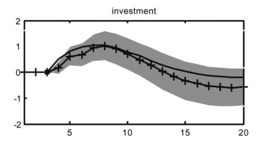
126 These plots are taken from Figure 1 of Christiano, Eichenbaum, Evans, JPE