Book Review: The Volatility Surface. A Practitioner s Guide (Jim Gatheral, Wiley-Finance, 2006)

Transcription

1 Book Review: The Volatility Surface. A Practitioner s Guide (Jim Gatheral, Wiley-Finance, 2006) Anatoliy Swishchuk University of Calgary Bankers Hall, Calgary, AB, Canada May 17, 2011 PRMIA Calgary Chapter s Talk

2 Book s Cover

3 Outline of Presentation 1. Introduction to the Book 2. Contents of the Book 3. Review of Chapters Short Description of Chapters Conclusion

4 Intro to the Book: About the Author Jim Gatheral is a Managing Director at Merrill Lynch and also an Adjunct Professor at the Courant Institute of Mathematical Sciences, New York University. Dr. Gatheral obtained a PhD in theoretical physics from Cambridge University in From 1997 to 2005, Dr. Gatheral headed the Equity Quantitative Analytics droup at Merrill Lynch. His current research focus is equity market microstructure and algorithmic trading.

5 Jim Gatheral s Picture

6 Intro to the Book: Purpose The purpose of The Volatility Surface is not to just present results, but to provide you with ways of thinking about and solving practical problems that should have many other areas of application.

7 Intro to the Book: Purpose Understandin the volatility surface is a key objective for both practitioners and academics in the field of finance.

8 Intro to the Book: Purpose Implied volatilities evolve randomly and so models of the volatility surface-which is formed from implied volatilites of all strikes and expirations-need to explicitele reflect this randomness in order to accurately price, trade, and manage the risk of derivative products.

9 Intro to the Book: Focus The first half of the book focuses on setting up the theoretical framework, while the later chapters are oriented towards practical applications.

10 Intro to the Book: Focus The Volatility Surface : Contains a detailed derivation of the Heston model and explanations of many other popular models such as SVJ, SVJJ, SABR, and CreditGrades Discusses the characteristics of various types of exotic options from the humble barrier option to the super exotic Napoleon

11 Contents of the Book Book contains: 11 Chapters Bibliography (74 sources) Index Many figures (47) 12 Tables

12 Chapters 1-3 Short Descriptions Chapter 1 Stochastic Volatility and Local Volatility : Provides an explanation of stochastic (SV) and local volatility (LV); local variance is shown to be the risk-neutral expectation of intantaneous variance, a result that is applied repeatedly in later chapters.

13 Chapters 1-3 Short Descriptions Chapter 2 The Heston Model : Presents the still supremely popular Heston model and derive the Heston European option pricing formula. It s also shown how to simulate the Heston model.

14 Chapters 1-3 Short Descriptions Chapter 3 The Implied Volatility Surface : Derives a powerful representation for implied volatility (IV) in terms of local volatility and applies this to build intuition and derive some properties of the impled volatility surface (VS) generated by the Heston model and compare with the empirically observed SPX surface; deduces that SV cannot be the whole story.

15 Chapters 1-3 Review Book s Cover

16 Chapter 1: Stochastic Volatility (SV) and Local Volatility (LV)

17 Structure of Chapter 1: Stochastic Volatility (SV) and Local Volatility (LV) 1. SV: Derivation of the Valuation Equation 2. LV: History, Brief Review of Dupire s Work 3. LV in Terms of Implied Volatility (IV) 4. LV as a Conditional Expectation of Instantaneous varinace

18 Chapter 1: Stochastic Volatility (SV) and Local Volatlity (LV) In this chapter, author introduces SV-the notion that volatility varies in a random fashion. LV then is then shown to be conditional expectation of the instantaneous variance so that various quantities of interest (such as option prices) may sometimes be computed as though future volatility were detrministic rather than stochastic.

19 Chapter 1: Stochastic Volatility (SV) Sense to model SV as a RV: observations of equity market (the stock market crash of October 1987). SV models are useful because they explain in a self-consistent way why options with different strikes and maturities have different Black-Scholes implied volatilities-that is, the volatility smile. Moreover, unlike alternative models that can fit the smile (such as LV models, e.g.), SV models assume realistic dynamics for the underlying.

20 Chapter 1: Stochastic Volatility (SV) Although SV price processes are sometimes accused by being ad hoc, on the contrary, they can be viewed as arising from Brownian motion subordinated to a random clock. This clock time, often referred to as trading time, may be identified with the volume of trades or the frequency of trading (Clark 1973); the idea is that as trading activity fluctuates, so does volatility.

21 Chapter 1: Stochastic Volatility (SV) From a hedging perspective, traders who use the Balck-Scholes model must continuously change the volatility assumption in order to match market prices. Their hedge ratios change accordingly in an uncontrolled way; SV models bring some order into this chaos. The prices of exotic options given by models based on Black- Scholes assumptions can be widely wrong and dealers in such options are motivated to find models that can take the volatility smile into account.

22 Chapter 1: Stochastic Volatility (SV) In Figure 1.1, the log returns of SPX over a 15-year period is plotted; we see that large moves follow large moves and small moves follow small moves (so-called volatility clustering ).

23 SPX Daily Log Returns (Dec 31, 1984-Dec 31, 2004)

24 Chapter 1: Stochastic Volatility (SV) In Figure 1.2, the frequency distribution of SPX log returns over the 77-year period from 1928 to 2005 is plotted. The distribution is highly peaked and fat-tailed relative to the normal distribution.

25 Frequency Distribution of 77 Years of SPX Daily Log Returns

26 Chapter 1: Stochastic Volatility (SV) The Q-Q plot in Figure 1.3 shows just how extreme the tails of the empirical distribution of returns are relative to the normal distribution. (This plot would be a straight line if the empirical distribution were normal).

27 Q-Q Plot of SPX Daily Log Returns

28 Chapter 1: Stochastic Volatility (SV) Fat tails and the high central peak are characteristics of mixtures of distributions with different variances. This motivates to model variance as a RV. The volatility clustering feature implies that volatility (or variance) is auto-correlated. In the model, this is a consequence of the mean revertion of volatility.

29 Chapter 1: Stochastic Volatility (SV) (Derivation of the Valuation Equation) In this section, author follows Wilmott (2000). Suppose that the stock price S and its variance v satisfy the following SDEs: with ds t = µ t S t dt + v t S t dz 1 dv t = α(s t, v t, t)dt + ηβ(s t, v t, t) v t dz 2 (1) dz 1, dz 2 = ρdt. (2)

30 Chapter 1: Stochastic Volatility (SV) (Derivation of the Valuation Equation) The process S t followed by the stock price is equivalent to the one assumed in the derivation of B-S (1973). This ensures that the standard time-dependent volatility version of the B-S formula (as derived in Sec. 8.6 of Wilmott (2000), e.g.) may be retrieved in the limit η 0. In practical applications, this is a key requirement of a SV option pricing model as practitioners intuition for the behaviour of option prices is invariably expressed within the framework of the B-S formula. No assumption wrt the form of functions α and β.

31 Chapter 1: Stochastic Volatility (SV) (Derivation of the Valuation Equation) In the B-S case, there is only one source of randomness, the stock price, which can be hedged with stock. In the present case, ranom changes in volatility also need to be hedged in order to form a riskless portfolio. So we set up a portfolio Π containing the option being priced, whose value we denote by V (S, v, t), a quantity of the stock and a quantity 1 of another asset whose value V 1 depends on volatility.

32 Chapter 1: Stochastic Volatility (SV) (Derivation of the Valuation Equation) Equation for V has the following form: V t vs2 2 V S 2 + ρηvβs 2 V v S η2 vβ 2 2 V v2 + rs V S rv = (α φβ v) V v, where we have written the arbitrary function of S, v, t as (α φβ v), where α and β are the drift and volatility functions from the SDE (1).

33 Chapter 1: Stochastic Volatility (SV) (Market Price of Volatility Risk) Function φ(s, v, t) is called market price of volatility risk. To see why, we follow Wilmott s argument. Consider the portfolio Π 1 consisting of a delta-hedged option V. Then Π 1 = V V S S and applying Itô s lemma and taking into account of deltahedged option (the coefficient of ds is zero), we have dπ 1 rπ 1 dt = β v V v [φdt + dz 2].

34 Chapter 1: Stochastic Volatility (SV) (Market Price of Volatility Risk) We see that the extra return per unit of volatility risk dz 2 is given by φdt and so in analogy with the CAPM, φ is known as the market price of volatility risk. Defining the risk-neutral drift as α = α β vφ we see that, as far as pricing of options is concerned, we could have started with the risk-neutral SDE for v, dv = α dt + β vdz 2 and got identical results with no explicit price of risk term because we are in the risk neutral world.

35 Chapter 1: Stochastic Volatility (SV) (Risk-Neutral World) In what follows, we always assume that the SDEs for S and v are in risk-neutral terms because we are invariably interested in fitting models to option prices. Effectively, we assume that we are imputing the risk-neutral measure directly by fitting the parameters of the process that we are imposing.

36 Chapter 1: Local Volatility (LV), History Given the computational complexity of SV models and difficulty of fitting parameters to the current prices of vanilla options, practitioners sought a simpler way of pricing exotic options consistently with the volatility skew. Since before Breeden and Litzenberger (1978), it was undestood that the risk-neutral density could be derived from the market prices of European options.

37 Chapter 1: Local Volatility (LV), History The breakthrough came when Dupire (1994) (continuous time version) and Derman and Kani (1994) (discrete time binomial tree version) noted that under risk neutrality, there was a unique diffusion process consistent with these distributions. The corresponding unique state-dependent diffusion coefficient σ L (S, t), consistent with current European option prices, is known as the local volatility function.

38 Chapter 1: Local Volatility (LV), History As if any proof were needed, Dumas, Fleming and Whaley (1998) performed an empirical analysis that confirmed that the dynamics of the implied volatility surface were not consistent with the assumption of constant local volatilities. Later on, we show that LV is indeed an average over instantaneous volatilites, formalizing the intuition of those practitioners who first introduced the concept.

39 Chapter 1: Local Volatility (LV): A Brief Review of Dupire s Work For a given expiration T and current stock price S 0, the collection C(S 0, K, T ) of undiscounted option prices of different strikes yields the risk-neutral density function φ of the final spot S T through the relationship C(S 0, K, T ) = K (S T K)φ(S T, T ; S 0 )ds T.

40 Chapter 1: Local Volatility (LV): A Brief Review of Dupire s Work Differentiate this twice wrt K to obtain φ(s T, T ; S 0 ) = 2 C K 2 so the Arrow-Debreu prices for each expiration may be recovered by twice differentiating the undiscounted option price wrt K.

41 Chapter 1: Local Volatility (LV): A Brief Review of Dupire s Work Given the distribution of final spot prices S T for each time T conditional on some starting spot price S 0, Dupire shows that there is a unique risk neutral diffusion process which generates these distributions. That is, given the set of all European option prices, we may determine the functional form of the diffusion parameter (LV) of the unique risk neutral diffusion process which generates these prices.

42 Chapter 1: Local Volatility (LV): A Brief Review of Dupire s Work Let us write the process as ds S = µ tdt + σ(s t, t; S 0 )dz. Application of Itô lemma together with risk neutrality, gives rise to a partial DE for functions of the stock price, which is a straightforward generalization of B-S. In particular, the pseudoprobability densities φ = 2 C K 2 must satisfy the Fokker-Planck equation.

43 Chapter 1: Local Volatility (LV): A Brief Review of Dupire s Work This leads to the following equation for the undiscounted option price C in terms of the strike price: C T = σ2 K 2 2 C 2 K 2 + (r t D t )(C K C K ), where r t is the risk-free rate, D t is the dividend yield and C is short for C(S 0, K, T ).

44 Chapter 1: Local Volatility (LV): Derivation of the Dupire Equation Here, φ is the pseudo-probability density of the final spot time T. It evolves according to the Fokker-Planck equation: S 2 T (σ 2 S 2 T ) S (µs T φ) S T = φ T.

45 Chapter 1: Local Volatility (LV): Derivation of the Dupire Equation Differentiting wrt K gives and C + K = ds T φ(s T, T ; S 0 ), K 2 C K 2 = φ.

46 Chapter 1: Local Volatility (LV): Derivation of the Dupire Equation Differentiating C wrt T (and taking into account above φ T ) gives { C + 1 T = 2 } ds T (σ 2 ST 2 K 2 ) S (µs T φ) (S T K). S T S 2 T Integrating by parts twice gives: C T = σ2 K 2 2 C C + µ(t )( K 2 K2 K ) which is the Dupire equation when the underlying stock has riskneutral drift µ.

47 Chapter 1: Local Volatility (LV): Derivation of the Dupire Equation That is, the forward price of the stock at time T is given by F T = S 0 exp( µ tdt). 0 Were we to express the option price as a function of the forward price F T, we would get the same expression minus the drift term. That is, T C T = 1 2 σ2 K 2 2 C K 2, where C = C(F T, K, T ).

48 Chapter 1: Local Volatility (LV): Derivation of the Dupire Equation Inverting this gives σ 2 (K, T, S 0 ) = C T 1 2 K2 2 C K 2 The right-hand side of the last equation can be computed from known European option prices. So, given a complete set of European option prices for all strikes and expirations, LVs are given by the last equation. We can view this equation as a definition of the LV function regardless of what kind of process (SV, e.g.) actually governs the evolution of volatility.

49 Chapter 1: Local Volatility (LV): LV in Terms of Implied Volatility (IV) Market prices of options are quoted in terms of B-S IV σ BS (K, T ; S 0 ). In other words, we may write C(S 0, K, T ) = C BS (S 0, K, σ BS (K, T ; S 0 ), T ). More convenient to work in terms of two dimensionless variables: the B-S implied total variance w defined by and the log-strike y defined by w(s 0, K, T ) := σ 2 BS (K, T ; S 0)T y = log( K F T ), where F T = S 0 exp( T 0 µ t dt) gives the forward price of the stock at time 0.

50 Chapter 1: Local Volatility (LV): LV in Terms of Implied Volatility (IV) In terms of these variables, the B-S formula for the future value of the option price becomes C BS (F T, y, w) = F T [N(d 1 ) e y N(d 2 )] = F T [N( y w + w 2 ) ey N( y w w 2 )] and the Dupire equation becomes C T = v L C 2 [ 2 y 2 C ] + µ(t )C y with v L = σ 2 (S 0, K, T ) representing the LV.

51 Chapter 1: Local Volatility (LV): LV in Terms of Implied Volatility (IV) Using Black-Scholes formula and Dupire equation we get: v L = w T 1 y w w y ( 1 4 w 1 + y2 w 2)( w y ) w y 2

52 Chapter 1: Local Volatility (LV): LV in Terms of Implied Volatility (IV): Special Case: No Skew If the skew w y is zero, we must have (see previous slide) v L = w T. So the LV in this case reduces to the forward B-S IV. The solution to this is w(t ) = T 0 v L(t)dt.

53 Chapter 1: Local Volatility (LV): LV as a Conditional Expectation of Instantaneous Variance This result was origimally independently derived by Dupire (1996) and Derman and Kani (1998). Follwing now the elegant derivation by Derman and Kani, assume the same stochastic process for the stock price ds t = µ t S t dt + v t S t dz but write it in terms of the forward price F t,t = S t exp[ T t µ s ds] : Note that df T,T = ds T. df t,t = v t F t,t dz.

54 Chapter 1: Local Volatility (LV): LV as a Conditional Expectation of Instantaneous Variance The undiscounted value of a European option with strike K expiring at time T is given by C(S 0, K, T ) = E Q [(S T K) + ]. Differentiating once wrt K gives K C = E Q[θ(S T K)], where θ is the Heaviside function. Differentiating again wrt K gives 2 C K 2 = E Q[δ(S T K)], where δ is the Dirac δ function. Now a formal application of Itô s lemma to the terminal payoff of the option (and using df T,T = ds T ) gives the identity d(s T K) + = θ(s T K)dS T v T S 2 T δ(s T K)dT.

55 Chapter 1: Local Volatility (LV): LV as a Conditional Expectation of Instantaneous Variance Taking conditional expectations of each side, and using the fact that F t,t is a martingale, we get dc = de Q [(S T K) + ] = 1 2 E Q[v T S 2 T δ(s T K)]dT. Also, we can write E Q [v T S 2 T δ(s T K)] = E Q [v T S T = K] 1 2 K2 E Q [δ(s T K)] = E Q [v T S T = K] 1 2 K2 2 C K 2.

56 Chapter 1: Local Volatility (LV): LV as a Conditional Expectation of Instantaneous Variance Putting this together, we get C T = E Q[v T S T = K] 1 2 K2 2 C K 2. Comparing this with the definition of LV, we see that σ 2 (S 0, K, T ) = E Q [v T S T = K]. That is, LV is the risk-neutral expectation of the instantaneous variance conditional on the final stock price S T being equal to the strike price K.

57 Chapter 2: The Heston Model Book s Cover

58 Chapter 2: The process (Heston (1993)) with dz 1 t, dz2 t = ρdt. ds t = µ t S t dt + v t S t dz 1 t dv t = λ(v t v)dt + η v t dz 2 t This is an affine process: the drifts and covariance are linear in S t and v t.

59 Chapter 2: The Heston Model (The valuation equation) V t vs2 2 V S 2 + ρηvs 2 V v S η2 v V v + rs V S rv = λ(v v) V v. Note that Gatheral has assumed that the original process is already in the pricing measure.

60 Chapter 2: The Heston Model (European option pricing) The valuation equation rewritten Consider a call option expiring at T with strike price K. Set x = ln F t,t K, where F t,t is the T -forward price of the stock index at time t. Set τ = T t. Write C(τ, x, v) = e rτ V (t, S, v).

61 Chapter 2: The Heston Model (European option pricing) C τ vc xx 1 2 vc x η2 vc vv + ρηvc xv λ(v v)c v = 0 with final time condition C(0, x, v) = K(e x 1) +. According to Duffie, Pan, Singleton (2000), we can look for the solution in the form C(τ, x, v) = K ( e x P 1 (τ, x, v) P 0 (τ, x, v) ).

62 Chapter 2: The Heston Model (European option pricing) P equations: for j = 0, 1 P j τ + 2 v P j x ( 1)j v P j 2 x + η2 v P j 2 v + ρηv 2 P j v x + (a b jv) P j v = 0 where a = λv and b j = λ jρη. Final time conditions: lim τ 0 P j (τ, x, v) = 1 {x>0}.

63 Chapter 2: The Heston Model (Fourier transforms) Set, for j = 0, 1, so that P j (τ, u, v) = P j (τ, x, v) = 1 2π R e iux P j (τ, x, v)dx, R eiux P j (τ, u, v)du.

64 Chapter 2: The Heston Model (Transformed equations) The P equations have constant coefficients in x, and transform into where v[α j P j β j P j v + γ P j v ] + a P j v P j τ = 0, α j = u2 2 iu 2 + iju β j = λ ρηj ρηiu γ = η2 2.

65 Chapter 2: The Heston Model (Transformed equations) We look for solutions of this in the form P j (τ, u, v) = e C j(τ,u)v+d j (τ,u)v P j (0, u, v).

66 Chapter 2: The Heston Model (European option pricing) The result is a set of Riccati equations for C j and D j : where C j τ = λd j; r ± j = β j ± β 2 j 4α jγ 2γ D j τ = γ(d j r + j )(D j r j ), =: β j ± d j η 2. Given that C j (0, u) = D j (0, u) = 0, Gatheral deduces D(τ, u) = r j where g j = r j /r+ j. 1 e d jτ 1 g j e d jτ ; C(τ, u) = λr j τ 2λ η 2 ln 1 g je d jτ 1 g j,

67 Chapter 2: The Heston Model (European option pricing The final step is to compute P j (τ, x, v) = π 0 R e C j(τ,u)v+d j (τ,u)v+iux iu du, and compute the option value via C(τ, x, v) = K ( e x P 1 (τ, x, v) P 0 (τ, x, v) ).

68 Chapter 2: The Heston Model (European option pricing) Next Picture: Black Scholes implied volatilities from Heston option prices

69

70 Chapter 2: Simulation) The Heston Model (European option pricing: The SDE again with dz 1 t, dz2 t = ρdt. ds t = µ t S t dt + v t S t dz 1 t dv t = λ(v t v)dt + η v t dz 2 t

71 Chapter 2: The Heston Model (European option pricing: Euler discretization) The variance process becomes v i+1 = v i λ(v i v) t + η v i tz. The convergence is extremely slow.

72 Chapter 2: The Heston Model (European option pricing: Milstein discretization) Incorporating higher order terms in the Itô-Taylor expansion leads to v i+1 = v i λ(v i v) t + η v i tz + η2 = ( vi + η 2 4 t(z2 1) tz ) 2 λ(vi v) t η2 4 t. The stock process should be discretized in terms of x i = log S i /S 0 : x i+1 = x i v i 2 t + v i tw, where E[ZW ] = ρ.

73 Chapter 3: The Implied Volatility Surface Book s Cover

74 Structure of Chapter 3: The Implied Volatility Surface Ch.1 Brief review Getting Implied Volatilities from Local Volatilities Local Volatility in the Heston Model Implied volatility in the Heston model The SPX Implied Volatility Surface

75 Chapter 3: Main objective - Ch.1 - how to compute local volatilities from implied volatilities - Ch.3 - how to compute implied volatilities from local volatilities: - estimate local volatilities generated by a given SV model using the fact that the local variance (LV) is a conditional expectation of instantaneous variance - given an SV model we can approximate the implied volatility surface - conversely, given the shape of an actual implied volatility surface we can deduce some characteristics of the underlying process

76 Chapter 3: 1. Getting implied volatilities from local volatilities - Understanding implied volatility - Ch.1 derived a formula for local volatility in terms of implied volatility - it is not an easy task to invert this formula - instead, by exploiting the work of Dupire (1998), derive a general path-integral representation of Black-Scholes implied variance

77 Chapter 3: 1. Getting implied volatilities from local volatilities - Understanding implied volatility - Using x t := log S t /S 0 we have: v K,T (t) = v L (x t, t)q(x t )dx t, where q(s t ) looks like a Brownian Bridge density for the stock.

78 Chapter 3: 1. Getting implied volatilities from local volatilities - Understanding implied volatility - This suggests that some Taylor expansion can be written for q (2nd order) and v L (first order) around the peak x t so one can approximate: v K,T (t) v L ( x t, t) so: σ BS (K, T ) 2 1 T T 0 v L ( x t )dt - In words, the BS implied variance of an option with strike K and maturity T is given approximately by the integral from 0 to T of the local variances along the path x t that minimizes the Brownian Bridge density q(x t ).

79 Chapter 3: 2. Local volatility in Heston model When µ = 0, we can rewrite the Heston model dynamics: dx t = v t /2dt + v t dz t dv t = λ(v t v)dt + ρη v t dz t + 1 ρ 2 η v t dw t where dw t and dz t are orthogonal. Eliminating v t dz t, we get: dv t = λ(v t v)dt + ρη(dx t + v t /2dt) + 1 ρ 2 η v t dw t Idea: Compute local variances for the Heston model and integrate local variances from valuation date to expiration date using the formula derived previously.

80 Chapter 3: 2. Local volatility in Heston model - The unconditional expected instantaneous variance at time t is: ˆv s := E[v s ] = (v 0 v)e λs + v - The expected total variance to time t is: ŵ t := T 0 ( 1 e λt ˆv s ds = (v 0 v) λ ) + vt Finally we need to compute u t := E[v t x T ].

81 Chapter 3: 2. Local volatility in Heston model - Under some assumptions the last term approaches zero: du t λ (u t v )dt + ρη x T ŵ T ˆv t dt with λ = λ ρη/2 and v = vλ/λ. The solution of this equation is: u T ˆv T + ρη x T ŵ T T 0 ˆv s e λ (T s) ds with ˆv s := (v ˆv)e λ s + v

82 Chapter 3: 2. Local volatility in Heston model - Since from Ch.1 σ 2 (K, T, S 0 ) = E[v T x T ], the above equation gives an accurate approximate for the local variance within the Heston model (extremely accurate when ρ = ±1). We see that in the Heston model, local variance is approximately linear in x : u T = E[v T x T ] = ˆv T + ρη x T ŵ T T 0 ˆv s e λ (T s) ds

83 Chapter Implied volatility in Heston model - Combining the results from 1 and 2 we can now compute the implied variance by integrating the Heston local variance along the most probable stock price path joining the initial stock price to the strike price at expiration. σ BS (K, T ) 2 1 T T σ 2 x t,t dt = 1 T T u t ( x t )dt 0 0

84 Chapter Implied volatility in Heston model - Substituting this into the equation for u T we have: σ BS (K, T ) 2 1 T T u t ( x t )dt 1 T 0 T 0 ˆv tdt + ρη x T 1 ŵ T T T 0 dt t 0 ˆv s e λ (t s) ds

85 Chapter 3: 3. Implied volatility in Heston model - The term structure of Black-Scholes Implied volatility in the Heston model - The at-the-money term structure of BS implied variance in the Heston model is obtained by setting x T = 0. σ BS (K, T ) 2 K=FT 1 T T 0 ˆv tdt = 1 T T 0 [(v v )e λ t + v ] dt = (v v ) 1 e λ T λ + v T - when T 0 the at-the-money BS implied variance converges to the level of instantaneous variance v and as T the atthe-money BS implied variance reverts to v.

86 Chpater 3: 4. The SPX implied volatility surface - the SVI parametrization - Gatheral (2004) proposes the following stochastic volatility inspired (SVI) parametrization for the volatility smile: σ BS (k) = a + b ( ρ(k m) + (k m) 2 + σ 2) where k is the log-strike and a, b, ρ, σ and m are some parameters depending on the expiration.

87 Chpater 3: 4. The SPX implied volatility surface - the SVI parametrization - Figure 1 below shows the surface from a nonlinear SVI fit to observed implied variance as a function of k for each expiration on September 15, 2005

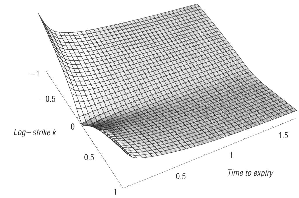
88

89 Chpater 3: 4. The SPX implied volatility surface - the SVI parametrization - Figure 2 below shows the SVI fit of the SPX implied volatilities for each of the eight listed expirations as of the close on September 15, Strikes are on the x-axis and implied volatilities are on the y-axis. The black and grey diamonds represent bid and offer volatilities respectively and the solid line is the SVI fit.

90

91 Chpater 3: 4. The SPX implied volatility surface - the SVI parametrization - Figure 3 below shows the plot of at-the-money skews as a function of time. The solid and dashed lines show the results of fitting the approximate formula: ρη 1 (1 λ 1 e λ T ) T λ T - The solid line takes all points into account while the dashed line drops the first three time to expirations - The observed variance skew increases faster as T 0 than the one implied by an SV model. Including jumps might solve the problem.

92

93 Chapter 3: 4. The SPX implied volatility surface - A Heston fit to the data - The parameters are: v = , v = , η = , ρ = and λ =

94 Chapter 3: 4. The SPX implied volatility surface - A Heston fit to the data - Figure 4 below shows a comparison between the empirical SPX implied volatility surface with the Heston fit on Nov 15. Heston fits well enough long maturity options, but does a poor job for short expirations. The upper surface is the empirical one. The Heston fit surface has been shifted down by five volatility points.

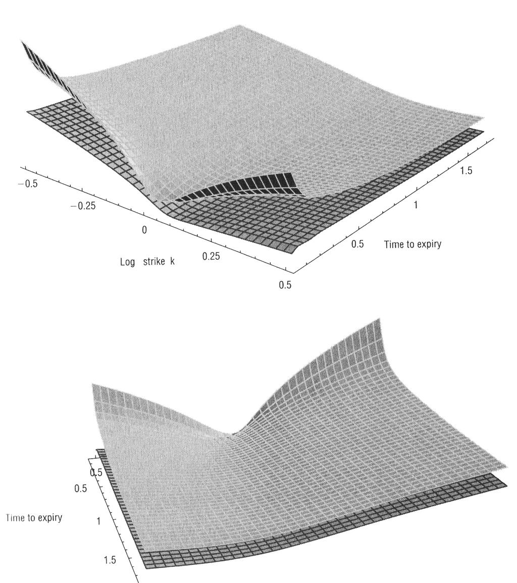
95

96 Contents of the Book: 4-11 Chapters Short Descriptions Book s Cover

97 Contents of the Book: 4-11 Chapters Short Descriptions Chapter 4 The Heston-Nandi Model : Chooses specific numerical values for the parameters of the Heston model, ρ = 1 as originally studied by Heston and Nandi and demonstartes that an approximate formula for implied volatility derived in Chapter 3 works particularly well in this limit. As a result, we are able to find parameters of LV and SV models that generate almost identical European option prices.

98 Contents of the Book: 4-11 Chapters Short Descriptions Chapter 5 Adding Jumps : Explores the modelling of jumps showing first why jumps are required; introduces then characteristic function techniques and applies these to the computation of IV in models with jumps; concludes by showing that the SVJ (SV with jumps in the stock price) is capable of generating a volatility surface that has most of the features of the empirical surface.

99 Contents of the Book: 4-11 Chapters Short Descriptions Chapter 6 Modelling Default Risk : Applies the work on jumps to Merton s jump-to-ruin model of default; explains the Credit- Grades model.

100 Contents of the Book: Chapters Short Descriptions Chapter 7 Volatility Surface Asymptotics : examines the asymptotic properties of the VS showing that all models with SV and jumps generate VS that are roughly the same shape.

101 Contents of the Book: 4-11 Chapters Short Descriptions Chapter 8 Dynamics of the Volatility Surface : shows how the dynamics of V can be deduced from the time series properties of VS; shows also why it is the dynamics of the VS generated by LV models are highly unrealistic.

102 Contents of the Book: 4-11 Chapters Short Descriptions Chapter 9 Barrier Options : presents various types of barrier options (BO) and shows how intuition may be developed for these by studying two simple limiting cases.

103 Contents of the Book: 4-11 Chapters Short Descriptions Chapter 10 Exotic Cliquets : studies in detail three actual exotic cliquet transactions that happen to have matured so that we can explore both pricing and ex post performance, specifically, a locally capped and globally floored cliquet, a reverse cliquet, and a Napoleon.

104 Contents of the Book: 4-11 Chapters Short Descriptions Chapter 11 Volatility Derivatives (the longest of all): focuses on the pricing and hedging of claims whose underlying is quadratic variation, explains why the market in volatility derivatives is suprisingly active and liquid.

105 Conclusion 1. Introduction to the Book 2. Contents of the Book 3. Chapters 1-3 Review 4. Chpaters 4-11 Short Description

106 Acknowledgements: Thank to all our faculty and grad students very much for doing review of this book at the Lunch at the Lab finance seminar (September 2010-March 2011): A. Badescu, D. Sezer, A. Ware, A. Gezahagne, K. Cui, K. Zhao, P. Dovoedo! Many thanks to MITACS for supporting our Lunch at the Lab finance seminar! (For all Chapters review see our Lunch at the Lab finance seminar s web:

107 Acknowledgements: Many thanks to Scott Dalton and PRMIA Calgary Chapter for the opportunity to give this talk!

108 Thank You for Your Time and Attention! Q&A Time!