Multi-factor Stochastic Volatility Models A practical approach

Transcription

1 Stockholm School of Economics Department of Finance - Master Thesis Spring 2009 Multi-factor Stochastic Volatility Models A practical approach Filip Andersson 20573@student.hhs.se Niklas Westermark 20653@student.hhs.se Abstract Since the legendary Black-Scholes (1973) model was presented, both academics and practitioners have made efforts to relax its assumptions and generate option pricing models that allow for non-normal return distributions and non-constant volatility. In this thesis, we examine the performance of four structural models ranging from the single-factor stochastic volatility model of Heston (1993) to a two-factor stochastic volatility model allowing for lognormally distributed jumps in the stock return process. We apply a practical view on the models by assuming that they are all to some degree misspecified. As a result, we do not pursue the classical route of trying to find the true model parameters using multiple crosssections in the model estimation, but estimate the models daily in order to find parameters that match today s market prices as closely as possible. The structural models are benchmarked against an ad-hoc Black-Scholes model, popular among practitioners. Our results show that adding an additional stochastic volatility factor to the return process significantly improves pricing performance, both in- and out-of-sample. We also show that the benefits of adding jumps to the return process are negligible in our sample, partly explained by the exclusion of very short-dated options. Lastly, we also provide some evidence on the estimation and implementation difficulties that are the drawbacks of the more sophisticated models. Tutor: Assistant professor Roméo Tédongap. Date and time: May 12 th 2009, 10:15. Location: Room 550. Discussants: Alok Alström and Anna Blomstrand. Acknowledgements: We would like to thank our tutor Roméo Tédongap for helpful advice during the writing of this thesis. We are also grateful to Misha Wolynski for valuable comments and suggestions and to Jacob Niburg for inspiring discussions.

2 Table of Contents 1. Introduction Purpose and research questions Theoretical framework Risk-neutral valuation Stock price dynamics Valuing options using characteristic functions and the Fast Fourier Transform Implied volatility and the volatility surface Previous research Stochastic volatility and jump models Multi-factor stochastic volatility models Local volatility models Other models Model introduction Stochastic volatility model (SV) Stochastic volatility model with jumps (SVJ) Multifactor stochastic volatility model (MFSV) Multifactor stochastic volatility model with jumps (MFSVJ) The Practitioner Black-Scholes model (PBS) Previous empirical findings Methodology Estimation Evaluation Data description Results Parameter estimates Pricing performance In-sample performance Out-of-sample performance Sub-sample analysis Estimation and implementation issues Conclusions References Appendix A: Figures and tables Appendix B: Volatility surface parameterization Appendix C: Derivation of the call price formula using characteristic functions and the FFT Appendix D: Data cleaning Appendix E: Estimation Appendix F: The approximate IV loss function i

3 1. Introduction Over 35 years have now passed since the publication of the famous Black & Scholes (1973) paper. Since then, an immense literature on option pricing theory has emerged in order to address the inconsistencies between the Black-Scholes model and empirical findings. In particular, the assumptions of normally distributed returns and constant volatility have been shown to be the major draw-backs of the model 1. As a result, academics and practitioners have tried to develop models that allow for non-normal return distributions and non-constant volatility. Models that allow negative correlation between the underlying stock price performance and its volatility are examples of such models that have become very popular in the literature. The development of more sophisticated models however comes at the cost of increased complexity. While the Black-Scholes model only has one unknown parameter (volatility), stochastic volatility models and further extensions often have between five and fifteen parameters. The increased parameterization imposes a risk of over-fitted models, with poor outof-sample performance as a consequence. Extensions of the original stochastic volatility models include multi-factor models, with two or more stochastic volatility factors. Previous literature has focused on the use of multi-factor models for capturing the variation in option prices or, equivalently, the implied volatility surface over long time periods, sometimes up to 10 years, with only one set of model parameters. The idea of using a long time period for model estimation may seem appealing from a theoretical point of view, as we expect the estimated model parameters to converge to the true parameters as the size of the sample gets sufficiently large. Convergence to true model parameters, however, relies on the assumption that there actually exist some true parameters or, in other words, that the model is correctly specified. Although this assumption is sometimes necessary in order to perform a meaningful analysis, it does not necessarily hold true. 1 See Hull (2006) for a description of the Black-Scholes model and Cont (2001) for some stylized facts on asset returns and volatility. 1

4 Christoffersen & Jacobs (2004) argue that all option pricing models are to some degree misspecified and, as a consequence, that the standard notion that a large enough sample will result in convergence to the true model parameters no longer is valid. The argument carries particular implications for practitioners. For traders, speculators and investors, the main objective of any option pricing model is to price options, as of today, as accurately as possible. The practical approach to option price modeling should thus be to find a model that, when incorporating all available information as of today, prices options as accurately as possible. In other words, as the notion of convergence to true model parameters is no longer valid, optimal model parameters should not be based on past information. In this thesis, we bring the practical approach to option price modeling to the field of multi-factor stochastic volatility models. We explore the subject by evaluating four structural option pricing models, ranging from a single-factor stochastic volatility model to a multi-factor stochastic volatility model that allows for log-normally distributed jumps in the return process of the underlying spot price. To further emphasize the practical perspective, the sophisticated structural models are compared to an ad-hoc Black-Scholes model, often referred to as the Practitioner Black-Scholes model. The models are applied to a universe of call options written on the EURO STOXX 50 index between January 1 st and December 31 st From the results, several interesting conclusions can be drawn. Partially contradicting the results of Christoffersen & Jacobs (2004), we find that the ad-hoc Black-Scholes model is outperformed by all structural models, especially out-of-sample. Furthermore, contrary to e.g. Bates (1996a, 2000) and Bakshi, Cao & Chen (1997), we do not find significant improvements in pricing performance of the structural models through the addition of jumps to the spot price process, not even in the short-maturity category. However, the addition of jumps does not make the models over-fitted, despite non-zero estimates of the jump factor parameters, and the out-of-sample results of the jump models are very similar to the jump free counterparts. On the other hand, expanding the parameter set by introducing additional stochastic volatility factors significantly increases pricing performance both in- and out-of-sample. Our results show that multi-factor models are not only of academic interest for explaining the long-term development of the implied volatility surface, but also carry significant interest to practitioners looking for accurate option pricing models. To complete the analysis we would 2

5 encourage further studies of multi-factor models using single cross-section estimation, in particular with regards to the topics of hedging and exotic option pricing. 2. Purpose and research questions The purpose of this thesis is to apply a practical view on the pricing performance of four structural option pricing models and to compare their performance to an ad-hoc Black-Scholes model. In order to pursue this route, some limitations must be discussed. First of all, one must decide on a finite number of models to consider. A reasonable approach is to make this choice either to include at least one model from a range of categories in order to draw conclusions about the relationship between model structure and performance. Alternatively, one could include a number of models from within the same category in order to evaluate the effect of expanding existing models. For the purpose of this thesis, we limit our attention to five option pricing models, four of which are structural stochastic volatility based models and one is a benchmark ad-hoc Black-Scholes model, popular among practitioners. Second, one must decide whether to look at pricing or hedging performance or, if possible, include both aspects. Pricing refers to the models abilities to price various options, ranging from plain vanilla calls and puts to exotic options with complicated pay-off structures 2. Hedging, on the other hand, refers to the models abilities to extract hedge parameters that can be used to manage already existing positions. In other words, hedging refers to the knowledge of which offsetting positions to engage in order to neutralize an option position s sensitivity to changes in underlying variables. The two aspects are both essential: pricing allows us to know the fair price at which to buy or sell an option and hedging allows us to manage the position once the trade has settled. Hence, any decision to engage in an option position will need input with regards to both pricing and hedging. In terms of modeling, the two characteristics are also closely connected. In simple models, such as e.g. the standard Black-Scholes model, where analytical formulas exist for the price of many options, hedge parameters can be easily obtained by differentiating the price function. In more 2 See Zhang (1998) for an overview of exotic options. 3

6 complex models, where hedge parameters have to be obtained numerically, the connection between pricing and hedging is perhaps even closer since the numerical derivative of the price function is attained by re-calculating the option price after imposing small changes in the underlying variables. In order to enable in-depth analysis within the limited scope of this thesis, we concentrate on the pricing aspects of model performance and leave hedging performance as a topic for further studies. We also restrict the analysis to the pricing performance of plain vanilla options for which reliable price data can be acquired. This can be viewed as a first step towards a complete evaluation of the models at hand, as any such evaluation must start at parameter estimation and vanilla option pricing, before engaging into the more sophisticated fields of hedging and exotic option pricing. Option pricing models exist in various degrees of complexity and model evaluation will always be subject to a trade-off between aspects such as pricing performance, robustness, estimation difficulties, transparency and speed. In order to provide a clear and structured evaluation of the models, we focus on answering the following three research questions: 1. Does increased model complexity enhance pricing performance? 2. Do market conditions, in terms of volatility, affect the relative performance of the models? 3. What problems arise when estimating and implementing the models? The first question focuses purely on the performance of the models with respect to pricing errors, and leads to a suggestion which model should be adapted if pricing performance is the only benchmark. The second question aims to investigate the robustness of the models, from which conclusions can be drawn about potential biases in the performance with respect to the chosen time period and the underlying index. The third question is of a more qualitative nature, as estimation difficulty and complexity are rather subjective attributes. The aim of this question is however to shed light on potential difficulties and issues arising when using the different models rather than an attempt to measure the level of complexity. 4

7 3. Theoretical framework Andersson & Westermark 3.1. Risk-neutral valuation Risk-neutral valuation dates back to Cox & Ross (1976) who extend the results of Black & Scholes (1973). Cox & Ross recognized that if it is possible to derive an analytical expression in the form of a differential or difference-differential equation that a contingent claim must satisfy, in which one model parameter does not appear, this parameter can be altered in the model to make the underlying asset earn the risk-free rate. The value of the claim can then be calculated as its expected value using the modified parameter discounted at the risk-free rate. Harrison & Kreps (1979) extended this analysis by introducing the theory of equivalent martingale measures. They show that Cox and Ross method of adjusting the model parameters is equivalent to changing probability measure from the real-world probability measure P to an equivalent martingale measure 3 Q, also referred to as the risk-neutral probability measure. Under the riskneutral measure, the price of a derivative can be expressed as: Π t = e r(t t) E Q t f S T (1.1) where f S T is the pay-off function of the derivative and r is the constant risk-free rate of return 4. We use the short-hand notation E t E F t, in which F t is a filtration containing all available information at time t. The existence of an equivalent martingale measure Q ensures that the price is arbitrage free. In case the measure is unique, we refer to the market as complete, in which case all derivatives can be replicated using other assets. This also implies that the arbitrage free price is unique (Björk, 2004). In layman s terms, the risk-neutral probability measure can be viewed as a different approach to modeling risk. Instead of compensating for risk through the use of a higher discount rate, the probabilities of good outcomes are adjusted to be more conservative, resulting in a lower expected value. Another way of looking at the risk-neutral probability measure is to imagine a 3 The term martingale measure arises from the fact that under Q, the discounted price process of the underlying asset is a martingale. Two probability measures P and Q are said to be equivalent if, on a measurable space Ω, F, P A = 0 Q A = 0 A F. 4 Under stochastic interest rates, the corresponding expression is Π t = E Q t e T t r s ds f S T. Note that the discount factor in this case must be inside the expectation brackets, as it is unknown at time t. 5

8 parallel world where all assets have exactly the same prices as in our world, but all investors are risk-neutral. Since risk-neutral investors only care about expected value, and thus discount all investments at the risk-free rate, the expected values of risky assets must be adjusted to be lower for asset prices to be equal to prices in the real world. Hence, in the risk-neutral world, probabilities of good and bad outcomes must differ from the corresponding real-world probabilities. The transformation from P to Q eliminates the issue of computing an appropriate discount rate to account for risk, as the risk-neutral expectation in (1.1) is discounted at the risk-free rate. The valuation problem is thus reduced to finding the distribution of S T under the equivalent martingale measure in order to evaluate the risk-neutral expectation of f S T Stock price dynamics In order to evaluate the expectation of f S T, some information about the distribution of S T must be known. Rather than making any assumptions about this distribution directly, it is most often obtained from modeling the asset price as following a continuous stochastic process. One example of a simple stochastic process is the geometric Brownian motion that the stock return is assumed to follow (under P) in the Black-Scholes model: ds t S t = μdt + ςdw t P (1.2) where μ and ς denote the drift and volatility, respectively. The Wiener process W t P has independent normally distributed increments, dw t P ~N(0, dt). Since the value of the stock is known today, the assumption of an underlying stochastic process of the stock return enables the derivation of a distribution of the stock price at some future time point. It is important to note the link between risk-neutral valuation and modeling of stock-price dynamics. Risk-neutral valuation requires that we use the stochastic process of the asset price under the risk-neutral measure, rather than under the real-world probability measure. In other words: the use of the stochastic process for option pricing requires the knowledge of the riskneutral model parameters. 6

9 Finding the risk-neutral model parameters can be approached in two different ways. One method is to assume a process of the stock price under the real-world probability measure and use historical stock price data to estimate the parameters of the model. This approach is however troublesome if the model contains some parameter that is difficult to observe, such as e.g. the market price of volatility risk. A more commonly used estimation method that mitigates this problem is to first derive the process under the risk-neutral measure and then estimate the parameters using observed option price data, disregarding the historical performance of the underlying stock price. The latter method has an advantage in particular when a model describes an incomplete market. Recall that in an incomplete market, the equivalent martingale measure is not unique and several arbitrage free prices exist. This does however not mean that derivatives can be priced arbitrarily: conditional on the prices observed on the market; only one arbitrage free price will exist. Hence, the real-world modeler will face the challenge of finding the particular equivalent martingale measure chosen by the market and calculate prices accordingly. However, using the latter method and calibrating the risk-neutral model directly to option prices observed results, as required, in parameters according to the markets choice of Q Valuing options using characteristic functions and the Fast Fourier Transform In order to find the distribution of S T, or enough information about it, characteristic functions can be used. The characteristic function of a random variable X is defined as: φ u = E e iux (1.3) where i refers to the imaginary unit, i.e. i = 1. The characteristic function is defined for all u and exists for all distributions. As implied by its name, the characteristic function characterizes the distribution uniquely in the sense that every random variable possesses a unique characteristic function (Gut, 2005). Hence, there is a one-to-one relationship between the characteristic function of a random variable and its distribution. Denoting by s T the natural logarithm of the terminal spot price of the underlying asset i.e. s T = ln S T, the characteristic function of s T under Q is: 7

10 φ T u = E Q e ius T = e ius T q T s T ds T R (1.4) where q T (s) denotes the risk-neutral density of s T. It turns out that if the characteristic function (1.4) is known analytically, semi-analytical expressions of vanilla option prices can be obtained through the application of Fourier analysis (see e.g. Bakshi, Cao & Chen, 1997; Bates, 1996a; Heston, 1993 and Scott, 1997). Assuming that the characteristic function of the log-stock price is known analytically 5, the price of plain vanilla options can be determined using the Fast Fourier Transform (FFT) method first presented by Carr & Madan (1999) 6. In this approach, the call price is expressed in terms of an inverse Fourier transform of the characteristic function of the log-stock price under the assumed stochastic process. The resulting formula can then be re-formulated to enable computation using the FFT algorithm that significantly decreases computation time compared to standard numerical methods. The pricing formula for European call options using the FFT method takes the form: where C T k = e αk π 0 e iξk ψ T ξ dξ (1.5) ψ T ξ = e rt φ T ξ α + 1 i α 2 + α ξ 2 + i 2α + 1 ξ (1.6) in which φ T ( ) denotes the characteristic function of s T, k denotes the log of the strike price and α is a damping parameter of the model. In order to calculate call prices, (1.5) is (after some modification) computed numerically using the FFT. Put prices are obtained using the put-call parity 7. The derivations of (1.5), (1.6) and the discrete form of (1.5) allowing for evaluation using the FFT are shown in Appendix C. 5 See e.g. Applebaum (2004), Carr & Madan (1999), Gatheral (2006) and Kahl & Jäckel (2005) for discussions of how to obtain the characteristic functions of different processes. 6 Alternative methods are suggested by e.g. Heston (1993) and Gatheral (2006) and extensions have been provided by e.g. Lee (2004) and Cont & Tankov (2004). 7 It is worth noting that the put-call parity relies on the assumption of no short-sale constraints. Hence, in cases when the underlying asset is a single stock or a smaller index, where short-sale possibilities are limited, methods with explicit put price formulas may be more appropriate. 8

11 3.4. Implied volatility and the volatility surface In the context of the Black-Scholes model, the price of a European option is a function of the the spot price (S t ), strike price (K), interest rate (r), time to maturity (T t), dividend yield (q) and volatility (ς). There is generally no disagreement on the values of the first five parameters, whereas the treatment of ς has become a science in itself. The Black-Scholes model assumes that ς is a constant, namely the volatility of the underlying asset. If the assumptions of the Black-Scholes model were true, the implied volatility, i.e. the volatility that makes the Black-Scholes price coincide with the market price 8, of options with the same underlying asset would be constant independent of both expiry time and strike price. It turns out, however, that the implied volatility varies both with regards to time to expiry and strike price. One reason for the variation in implied volatility over different maturities, referred to as the volatility term structure, is that volatility is considered to be mean-reverting (Cont, 2001). Hence, when current volatility is low with respect to historical values, the volatility term structure tends to be upward-sloping, implying that investors expect volatility to increase, and vice versa. The term structure of volatility is also event-driven in the sense that implied volatilities will be higher for short maturities when there is an upcoming event that is likely to largely affect the stock price. Rubinstein (1994) found that the assumption of constant implied volatilities over all strike prices was fairly correct until the stock market crash in Since then, the implied volatility as a function of the strike price, called the volatility skew, typically has a form seen in Figure 1 below. Rubinstein suggested crash-o-phobia as an explanation to this, meaning that traders price out-of-the-money (OTM) puts and in-the-money (ITM) calls relatively higher than ITM puts and OTM calls, in order to protect themselves against the risk of a new stock market crash. Another observation, shown by e.g. Black (1976), is that the risk of a company increases with leverage. As equity decreases, the volatility increases due to the higher risk, and vice versa. In that context, the volatility is expected to be a decreasing function of price, which in turn gives rise to the common smirk shape of the volatility skew (Figlewski & Wang, 2000). 8 Since all other parameters are assumed to be known, the price essentially only depends on ς. Hence, for a given market price, we can solve for the value of sigma that makes the model price equal the market price. 9

12 Figure 1 below shows the volatility skew and term structure for the EURO STOXX 50 index as of July 17 th Skew plots for all maturities on the same date are shown in Appendix B. As can be seen, both plots confirm that the assumption of constant volatility over different strike prices and maturities is inconsistent with observed implied volatilities in the market. Hence, regardless of choice of ς, the Black-Scholes model will be unable to replicate market prices as a constant ς implies a horizontal line in both plots. Figure 1 Volatility skew and term structure of EURO STOXX 50 on July 17 th 2008 The left plot shows how the implied volatility decreases with strike price for call options with 32 days to maturity. The right plot shows how the implied volatility differs between ATM options with different maturities. Both plots are conflicting with the Black-Scholes assumption of constant volatility. In order to study the implied volatility patterns in more detail, it is necessary to look at the term structure for every strike price, as well as the skew for every maturity simultaneously. To incorporate all available information with regards to both term structure and skew, we would thus need one graph for each strike price showing the term structure, as well as one graph for each maturity displaying the skew. The problem is readily solved by showing the implied volatility as a two-variable function of time and strike price in a 3D-graph. The resulting surface is referred to as the volatility surface, and shows all available information with regards to term structure and skew at a given time point. Figure 2 below shows the volatility surface of the EURO STOXX 50 index as of July 17 th The surface is obtained by interpolation of the skew plots shown in Appendix B, where the calibration procedure is also described in detail. 10

13 Figure 2 Volatility surface of EURO STOXX 50 July 17 th 2008 The plot shows the implied volatility (calculated from option prices) at the specific date for days to maturity and strike price. The surface is obtained by interpolating the skew plots from Appendix B. The volatility surface plays an important role in the pricing of options. The first step towards a useful pricing model is that the model is able to replicate plain vanilla prices observed in the market. This is essentially equivalent to matching the observed implied volatilities, i.e. the market s volatility surface. Obviously, the Black-Scholes model is unable to accomplish this, as volatility in the Black-Scholes model is assumed to be constant for all maturities and strikes, implying a flat volatility surface. 4. Previous research In this section, we present previous research on stochastic volatility models, jump models, multifactor models and local volatility models. A summary of the empirical performances of the models are presented at the end of Section 5, after the models used in this thesis have been presented in more detail. 11

14 4.1. Stochastic volatility and jump models In stochastic volatility models, the volatility in addition to the stock price, is allowed to develop according to a stochastic process. Many different models have been proposed with the common property that volatility is modeled by its own diffusion process 9. In order to find a reasonable diffusion model for volatility, one must first consider some empirical facts of asset returns and volatilities. As mentioned, one of the most well-known properties of volatility is that it tends to be high in bear markets and low in bull markets, partially explained by the leverage effect. The negative correlation to asset returns is very important in the modeling of option prices, as it allows the model to generate the empirically observed volatility smirk. Additional well-documented properties that affect the prices of options and should be incorporated into any plausible stochastic volatility model, pointed out by e.g. Gatheral (2006), are volatility clustering and mean-reversion. Many stochastic volatility models, such as the Heston (1993) model indeed encompass these features. One short-coming of the stochastic volatility models is, however, their inability to capture the large short-term movements of stock prices that are observed frequently in the market. To this end, so called jump-diffusion models have been developed. The idea of adding a jump factor to the modeling of stock prices is not a new idea, but was introduced by Merton (1976) 10 short after the publication of the Black-Scholes model. The jump feature especially enables the model to explain the probabilities of large short-term moves in the stock price implied by far out-of-the money bid prices. Gatheral (2006) shows examples of 5 cent bid prices for 67 % OTM call options expiring the following morning, implying that traders are willing to pay 5 cents for options that, under normally distributed returns, have zero (to about 40 decimal places) probability of ending up in the money. Stochastic volatility models without jumps are unable to capture this implied probability of large short-term moves, and produce lower implied volatilities, and thus lower prices, for far OTM options with short maturities compared to observed prices in the market. Allowing for jumps is one way of mitigating this 9 See e.g. Hull & White (1987), Johnson & Shanno (1987), Melino & Turnbull (1990), Scott (1987), Stein & Stein (1991) and Wiggins (1987), although some of these models are obsolete in light of more recent models. 10 Merton s model is however a pure jump model, i.e. a model with deterministic volatility. 12

15 problem, as it will incorporate a certain probability of large instantaneous moves in the stock price. Several different jump-models have been proposed, with and without stochastic volatility, and with different distributions of the jump size. Cox, Ross & Rubinstein (1979) suggest a pure jump model with constant jump size, whereas Merton (1976) proposes a pure jump model with lognormally distributed jump size. Extensions of the latter include Bates (1996a) who incorporates stochastic volatility as well as log-normally distributed jumps in the stock price process. Zhu (2000) conducts an extensive analysis of option pricing models, including models with lognormally distributed jumps, Pareto distributed jumps and different types of stochastic volatility diffusion processes Multi-factor stochastic volatility models Bates (2000) and Christoffersen, Heston & Jacobs (2009) both propose two-factor stochastic volatility models as an alternative or extension to jump models in order to model the evolution of the implied volatility surface. The rationale behind the multi-factor model is that it is able to capture both long- and short-term movements in the volatility process. This enables the model to explain differences in both level and slope of the implied volatility surface over time. Christoffersen, Heston & Jacobs (2009) highlight that the two-factor model has a particular advantage when estimating models using multiple cross-sections of options, as the one-factor model will suffer from structural problems when the slope and level of the implied volatility surface change simultaneously over time. The model of Bates (2000) also allows for lognormally distributed jumps in the stock price process, in addition to having two stochastic volatility factors. This extension is natural, as jumps and multiple stochastic volatility factors serve different purposes and thus should not necessarily be seen as substitutes Local volatility models In local volatility models also referred to as deterministic volatility function models the volatility of the underlying asset is assumed to be a function of the level of the spot price and calendar time, i.e. ς t = ς(s t, t). In continuous time, the risk-neutral stock return process in the local volatility framework is hence of the form: 13

16 ds t S t = (r q)dt + ς S t, t dw t Q (4.1) where r and q denote the interest and dividend yield, respectively. The local volatility model was introduced in a discrete setting (using an implied tree method) by Derman & Kani (1994) and Rubinstein (1994), and extended to continuous time by Dupire (1994). The local volatility function ς t = ς(s t, t) is derived to make the model consistent with observed market prices or, equivalently, consistent to the observed implied volatility surface (see e.g. Rebonato (1999) for the derivation of the local and the relation to implied volatility). Since ς t is a function of a stochastic quantity (S t ), ς t will also be stochastic. Local volatility models differ from many other option pricing models in the sense that the purpose not is to model the actual evolution of the implied volatility surface, but rather provide a (not as harsh as Black & Scholes ) simplification in order to enable pricing of options consistent with existing prices of vanilla options (Gatheral, 2006). The notion is confirmed by Dumas, Fleming & Whaley (1998) who conclude that the local volatility model is unable to explain the empirical dynamics of the implied volatility surface. Instead, Dumas, Fleming & Whaley propose a different type of deterministic volatility function model, in which a function of strike price and maturity, i.e. ς t = ς(k, T t), is fitted to the observed implied volatility surface. Obviously, this function cannot be inserted into the stock price process, as doing so would lead to different processes for the same underlying stock depending on the strike price and maturity of the option at hand. Instead, the function is used to derive the implied volatility of non-traded options in order to enable pricing using the standard Black-Scholes formula Other models Eraker (2004) extends the modeling of stochastic volatility to allow for jumps also in the volatility process, following in the tracks of Bates (2000) who concludes that volatility jump models are necessary for capturing the volatility shocks observed in the S&P 500 futures market. Other popular models include the variance-gamma model, proposed by Carr, Chang & Madan (1998), in which the stock price return follows a geometric Brownian motion conditional on the realization of a gamma-distributed random time. Extensions of the variance-gamma model, put 14

17 forward by e.g. Carr, Geman, Madan & Yor (2001), include models where the underlying stock price is allowed to follow other Levý processes 11, driven by stochastic clocks. 5. Model introduction In this section, we introduce the models under evaluation in more detail. For each model, we provide some intuition to the features of the model making it appealing for option pricing and, where relevant, specify the assumptions of the underlying stock price process and the corresponding characteristic function of the log-stock price. The presentation, especially with regards to the characteristic functions, is in some parts rather technical, but the reader finding it difficult to interpret the technical details may pass those parts over without any substantial loss in intuition. For all models, we consider the risk-neutral dynamics of the stock price. We let S = S t, 0 t T denote the stock price process and V = {V t, 0 t T} denote the stochastic variance process. φ T ( ) denotes the characteristic function of the natural logarithm of the terminal stock price s T = ln S T. The constants r and q will denote the, both constant and Q continuously compounded, interest rate and dividend yield, respectively. Further, we let W t denote a Q-Wiener process Stochastic volatility model (SV) Allowing for the volatility of the stock price to be stochastic by itself is a well-known way of mitigating the aforementioned problems in the underlying assumptions of the Black-Scholes model. Stochastic volatility obviously allows for non-constant volatility, and also permits nonnormal distributions of returns. Many different stochastic volatility models have been proposed, but we will limit our attention to the Heston (1993) stochastic volatility model, henceforth denoted SV, in which the spot price is described by the following stochastic differential equations (SDEs) under Q: 11 See Applebaum (2004) for more on applications of Lévy processes in finance. 12 A Q-Wiener process is a process that fulfills the requirements of a Wiener process under the equivalent martingale measure Q. See Björk (2004) for a more detailed description of Wiener processes. 15

18 ds t S t = r q dt + V t dw t Q (1) dv t = κ θ V t dt + ς V t dw t Q 2 (5.1) (5.2) Cov t dw t Q 1, dwt Q 2 = ρdt (5.3) where the parameters κ, θ and ς represent the speed of mean reversion, the long-run mean and the volatility of the variance, and ρ represents the correlation between the variance and stock price processes, respectively. In addition to these parameters, the model requires the estimation of the instantaneous spot variance V 0. Pricing of plain-vanilla call options using the SV model can be done in several ways. Heston (1993) proposes a closed-form solution for the call price, also implemented and extended by e.g. Gatheral (2006). The closed form solution however requires numerical evaluation of the integral obtained from inversion of the characteristic function, and does thus not have the computational advantage of closed-form solutions that can be evaluated analytically (such as e.g. the Black- Scholes model). In order to minimize computation time, we will instead use the method of Carr & Madan (1999), described in Section 3 and Appendix B, and price options using the Fast Fourier Transform (FFT). Albrecher, Mayer, Schoutens & Tistaert (2006) show that the characteristic function of s T in the SV model requires some consideration in order to avoid numerical problems when pricing vanilla options using Fourier methods 13. The characteristic function of the SV model, regardless of specification, includes a logarithm of complex numbers. The numerical problem, first recognized by Schöbel & Zhu (1999), arises due to the fact that the logarithm function is discontinuous in its imaginary part along the negative real axis. Hence, in order to avoid discontinuities, it is important that the argument of the logarithm function does not cross the negative real axis, which Albrecher, Mayer, Schoutens & Tistaert show can be achieved by re-formulating the characteristic function. Hence, we deviate from the original characteristic function proposed by Heston (1993) and instead use the alternative formulation proposed by Albrecher, Mayer, 13 Kahl & Lord (2006) provide an alternative proof using a rotation count algorithm presented by Kahl & Jäckel (2005). Their conclusion is however identical to that of Albrecher, Mayer, Schoutens & Tistaert, namely that the proposed representation mitigates the problems of the original characteristic function in Heston (1993). 16

19 Schoutens & Tistaert. Using the same representation of the parameters as in equations (5.1) (5.3), the characteristic function of s T takes the following form: where φ T SV u = S 0 iu f(v 0, u, T) (5.4) f V 0, u, T = exp A u, T + B u, T V 0 (5.5) A u, T = r q iut + κθ 1 ge dt (κ ρςiu d)t 2 ln ς2 1 g B u, T = (5.6) κ ρςiu d 1 e dt ς 2 (5.7) 1 ge dt d = ρςiu κ 2 + ς 2 (iu + u 2 ) (5.8) g = (κ ρςiu d)/(κ ρςiu + d) (5.9) The derivation of (5.4) is rather complicated and is thus omitted. The interested reader is referred to Gatheral (2006) or Kahl & Jäckel (2005). Vanilla call prices in the SV model are calculated by substituting the characteristic function (5.4) into the Carr & Madan (1999) pricing formula (1.5) and evaluating using the FFT. The SV model also allows for straightforward pricing of exotic options using Monte Carlo simulation. Once the parameters have been estimated, sample paths of the process (5.1) can be simulated, allowing for the pricing of any contingent claim Stochastic volatility model with jumps (SVJ) We extend the SV model in the previous section along the lines of Bates (1996a), by adding lognormally distributed jumps to the stock price process. In this model, denoted SVJ, the return process of the spot price is described by the following set of SDEs under Q: ds t S t = r q λμ J dt + V t dw t Q (1) + Jt dy t (5.10) dv t = κ θ V t dt + ς V t dw t Q 2 (5.11) Cov t dw t Q 1, dwt Q 2 = ρdt (5.12) where Y = Y t, 0 t T is a Poisson process with intensity λ > 0, i.e. Q dy t = 1 = λdt and Q dy t = 0 = 1 λdt, and J t is the jump size conditional on a jump occurring. All other 17

20 parameters are defined as in (5.1) (5.3). The subtraction of λμ J in the drift term compensates for the expected drift added by the jump component, so that the total drift of the process, as required for risk-neutral valuation, remains (r q)dt. As mentioned, the jump size is assumed to be log-normally distributed: ln 1 + J t ~ N ln 1 + μ J ς J 2 2, ς J 2 (5.13) Q (1) Further, it is assumed that Y t and J t are independent of each other as well as of W t Q and W (2) t. In the SVJ model, the total variance of the return depends both on V t and on the variance added by the jump factor. Denoting the variance added by the jump component V J,t, the total variance of the return process equals (Bakshi, Cao & Chen, 1997): where Var t ds t S t = V t dt + V J,t dt (5.14) V J,t = Var t J t dy t = λ μ J 2 + e ς J μ J 2 (5.15) It should also be noted that the SVJ model nests the SV model, as choosing λ = μ J = ς J = 0 will reduce the SVJ model to the SV model 14. Hence, we would expect the SVJ model to always outperform the SV model in-sample. Out-of-sample, however, its performance is not necessarily superior to the SV model due to the risk of over-parameterization (a hazard that will re-appear as we expand the parameter set even further). Following the independence between Y t, J t and the two Wiener processes, it can be shown (see e.g. Gatheral, 2006 or Zhu, 2000) that the characteristic function of the SVJ model is: φ SVJ T (u) = φ SV T (u) φ J T (u) (5.16) where: 14 In fact, setting λ = 0 or μ J = ς J = 0 is sufficient, as both cases eliminate the effect of the jump component. 18

21 φ T J = exp[ λμ J iut + λt((1 + μ J ) iu exp(ς J 2 (iu/2)(iu 1)) 1)] (5.17) and φ SV T (u) is defined as in (5.4). As in the SV model, vanilla call prices can be obtained using the FFT method and exotic option prices can be calculated using Monte Carlo simulation Multifactor stochastic volatility model (MFSV) Christoffersen, Heston and Jacobs (2009) propose a two-factor stochastic volatility model as an alternative extension to the Heston (1993) SV model. They argue that the two-factor model is able to capture the time-variation in the volatility smirk better than the one-factor SV model. In particular, this will prove to be effective when the model is estimated using multiple crosssections of options (Christoffersen, Heston & Jacobs use daily option data during one year for each estimation), as the one factor model will be unable to capture the variation in the slope and level of the volatility smile over time. In light of the observation that the slope and level of the volatility smile often differ substantially between maturities even in a single cross-section, the multi-factor model will likely provide a better fit even in that setting. Hence, it is of interest to examine if the multi-factor model is able to outperform the SV model also in a one-dimensional cross-section. In particular, the out of sample performance will be of interest, since the addition of parameters might lead to overparameterization. We denote the multi-factor stochastic volatility model MFSV and let the following set of SDEs describe the return process under the risk-neutral measure: ds t S t = r q dt + V t (1) dwt Q (1) + V t (2) dwt Q (2) (5.18) dv t 1 = κ1 θ 1 V t 1 dv t 2 = κ2 θ 2 V t 2 dt + ς 1 V t 1 dwt Q 3 (5.19) dt + ς 2 V t 2 dwt Q 4 (5.20) where the parameters have the same meaning as in (5.1) (5.3). 19

22 The dependence structure is assumed to be as follows: Cov dw t Q 1, dwt Q 3 Cov dw t Q 2, dwt Q 4 = ρ 1 dt (5.21) = ρ 2 dt (5.22) Cov dw t Q i, dwt Q j = 0, i, j = 1,2, 1,4, 2,3, (3,4) (5.23) In other words, each variance process is correlated with the corresponding Wiener process in the return process, i.e. the diffusion term of which the respective variance process determines the magnitude. The dependence structure also implies that the total variance of the spot return equals the sum of the two variance factors, i.e. Var t ds t S t = V t 1 + Vt 2 dt (5.24) We obtain the characteristic function of the terminal log-stock price in the MFSV model by applying the methodology of Albrecher, Mayer, Schoutens & Tistaert (2006) to the characteristic function presented in Christoffersen, Heston & Jacobs (2009), extending it to allow for a continuous dividend yield q. The result follows by recognizing that the MFSV process (5.18) is the sum of the SV process (5.1) and an additional stochastic volatility term. By the independence of the two Wiener processes in the return process with respect to each other as well as each other s diffusion processes, the added term is independent of the nested SV model return SDE. Since the characteristic function of the sum of two independent variables is the product of their individual characteristic functions, the characteristic function of the MFSV model is determined as: φ T MFSV (u) = E 0 Q e ius T = S 0 iu f V 0 1, V0 2, u, T (5.25) where: f V 0 1, V0 2, u, T = exp A u, T + B1 u, T V B2 u, T V 0 2 (5.26) A u, T = r q iut + 2 j =1 ς j 2 κ j θ j κ j ρ j ς j iu d j T 2 ln 1 g j e d j T 1 g j (5.27) B j u, T = ς 2 1 e d j T j (κ j ρ j ς j iu d j ) 1 g j e d j T (5.28) 20

23 g j = κ j ρ j ς j iu d j κ j ρ j ς j iu + d j (5.29) d j = ρ j ς j iu κ j 2 + ς j 2 (iu + u 2 ) (5.30) The existence of a closed form characteristic function makes pricing in the MFSV model no more difficult than in the SV and SVJ models. The potential problem, as discussed in context of the SVJ model, arises out of sample as the model might suffer from over-parameterization. It is however important to notice that the MFSV model does not nest the SVJ model. Hence, it is possible for the SVJ model to outperform the MFSV model even in-sample Multifactor stochastic volatility model with jumps (MFSVJ) As explained in the context the SVJ model, jumps help the model explain the implied probability of large short-term movements in the underlying stock price. Adding jumps thus enables the model to better price far out of the money options with short expiry times. Hence, as jumps serve a different purpose than the additional stochastic volatility factor in the MFSV model, adding jumps might enhance the performance of the MFSV model. Obviously, the jump factor extends the parameter set of the model even further, and the aforementioned potential problem of overparameterization arises once more, making out-of-sample performance vital for assessing the model s performance. In the MFSVJ model, the risk-neutral stock price dynamics are described by the following set of SDEs: ds t S t = r q λμ J dt + V t (1) dwt Q (1) + V t (2) dwt Q (2) + Jt dy t (5.31) dv t 1 = κ1 θ 1 V t 1 dv t 1 = κ2 θ 2 V t 2 dt + ς 1 V t 1 dwt Q 3 (5.32) dt + ς 2 V t 2 dwt Q 4 (5.33) where all parameters and variables are defined as in equations (5.1) (5.3) and (5.10). The distributions of J t and Y t are log-normal and Poisson, respectively, according to equations (5.10) and (5.13), and the two variables are independent, both of each other and of the four Wiener 21

24 processes. The dependence structure between the Wiener processes is the same as in the MFSV model according to equations (5.21) (5.23). Given the total spot return variances of the SVJ and MFSV models, the total return variance of the MFSVJ can easily be established as: Var t ds t S t = V t 1 + Vt 2 dt + V J,t dt (5.34) where V J,t is defined as in equation (5.15). Due to the independence between the added jump factor and the SDE of the MFSV model, the characteristic function of s T is obtained in the same way as in the SVJ model, i.e. as the product of the jump-term characteristic function and the characteristic function of the MFSV model: φ MFSVJ T (u) = φ MFSV T (u) φ J T (u) (5.35) where φ T MFSV (u) and φ T J u are defined in (5.25) and (5.17), respectively The Practitioner Black-Scholes model (PBS) The PBS model originates from local volatility models in which the volatility is described as a deterministic function of time and the underlying stock price. Dumas, Fleming & Whaley (1998) find that local volatility models perform worse than an ad hoc method that smoothes implied volatilities from option data and then uses the traditional Black-Scholes pricing formula with the fitted implied volatilities. It is the latter method that is often referred to as the Practitioner Black- Scholes model (PBS), due to its popularity among practitioners. The difference between local volatility models and the PBS model is that the volatility in the PBS model is a function of strike price and time to maturity, rather than the spot price and calendar time. Christoffersen & Jacobs (2004) confirm the PBS models validity and find that, in their sample, the PBS model actually outperforms the more advanced stochastic volatility model of Heston (1993). Berkowitz (2001) provides a mathematical justification for the use of the PBS model and shows that the PBS model, when re-calibrated sufficiently frequently to a large number of options, will become arbitrarily accurate. 22

25 The PBS model is implemented by fitting a deterministic function of strike price and time to maturity to observed implied volatilities in the market. Several functions of different complexity have been proposed, but we will constrain our study to the most general function proposed by Dumas, Fleming & Whaley (1998), also used by Christoffersen & Jacobs (2004): ς = α 0 + α 1 K + α 2 K 2 + α 3 T + α 4 T 2 + α 5 KT (5.36) Plain vanilla call and put prices in the PBS model are simply calculated through the standard Black-Scholes formula using the implied volatility obtained from the fitted function (5.36) by inserting the strike price and time to maturity. As the implied volatility surface is under constant change, the model must be recalibrated at certain time intervals in order assure acceptable accuracy. Due to the straight-forward pricing method using the standard Black-Scholes formula, this is fairly simple and not very computer intensive, and can be done in a matter of minutes, or even seconds, depending on the number of options at hand Previous empirical findings In Table 1 below, we present a summary of previous studies on the empirical performance of the introduced models. It should be noted that the findings presented in the table are those relevant for the subject of this thesis, and thus not necessarily the main general results of the articles. In the table, the parameter time span refers to the time period used for estimation of the parameters. For example, a model estimated using one day s option data will have daily time span, whereas a model estimated using an option universe from a time period of one year will have an annual time span. The stochastic volatility model with jumps (SVJ) was, as mentioned, introduced by Bates (1996a), and has been the focus of several succeeding studies. Papers studying jump factors often discuss the importance of jumps in both returns and volatility, where the latter jump factor will increase explanatory power for time varying volatility. Eraker, Johannes & Polson (2003) is the only paper that supports jumps in volatility, while most other papers find this jump factor redundant. Eraker (2004) is the only paper finding both jump factors redundant, while most other papers conclude that the return jump factor increases in-sample performance. However, the effect 23

26 on out-of-sample performance is found to be very small. Broadie, Chernov & Johannes (2007) show that the addition of jumps significantly improves the performance of stochastic volatility models when certain parameters are restricted based on historical estimates. Two possible explanations to why the results regarding the jump factor are different across the previous research are given by Broadie, Chernov & Johannes (2007) and Eraker (2004). Broadie, Chernov & Johannes suggest the fact that the different papers use different sample periods, number of options per cross-section and test statistics, while Eraker points to the difference between using historical returns or option prices for model estimation. Christoffersen, Heston & Jacobs (2009) show that the MFSV model performs better both in- and out-of-sample than the SV model, indicating that adding additional stochastic volatility factors to the underlying stock price process is desirable. They however argue that the main benefits of adding a second stochastic volatility factor arise when the model is estimated using multiple cross-sections, as the parameter estimates are then required to be valid throughout a varying volatility environment. To the best of our knowledge, the only study elaborating on models with several stochastic volatility factors as well as jumps is Bates (2000), who however conducts his analysis using annual estimation of the model parameters, consistent with the argumentation of Christoffersen, Heston & Jacobs (2009) that multi-factor models are mainly suited for estimation using multiple cross-sections of options. As expected, the in-sample errors of the multi-factor models in Bates study are lower than their single-factor counterpart, but he does not perform any out-of-sample analysis from which further conclusions can be drawn. The main conclusion is rather that multifactor stochastic volatility models and jump models produce more plausible parameter estimates than single-factor stochastic volatility models, indicating that the out-of-sample performance of these models ought to be superior to the SV model. Dumas, Fleming & Whaley (1998) find that the PBS model outperforms the binomial tree models of Rubinstein (1994) and Derman & Kani (1994), in which the trees are fitted to exactly match observed implied volatilities introducing a severe over-fitting problem. Christoffersen & Jacobs (2004) discuss the importance of the loss function in estimation and evaluation, and use the PBS and SV models to illustrate their point. Their results with respect to the relative performance of 24

27 the models are inconclusive and depend on the loss function used for estimation and evaluation, but their results still show that the PBS model is a viable competitor to stochastic volatility models. The authors however do not make any comparison of the models using the implied volatility loss function used in this thesis (presented in the next section). Table 1 Summary of previous studies The table below summarizes previous findings on the empirical performance of the models used in this thesis. The findings are the ones relevant for the purpose of this thesis, and not necessarily the main result of each paper. Paper Data / Time period Parameter time span Findings Bates (1996a) Bakshi, Cao & Chen (1997) Dumas, Fleming &Whaley (1998) Bates (2000) Andersen, Benzoni & Lund (2002) Pan (2002) Deutsche Mark call and put options (USD) years SVJ more efficient than SV in modeling return distributions. SV cannot explain the volatility smirk, except under implausible parameters. S&P 500 call options day Stochastic volatility of first importance for model (SV). Further performance improvement when jumps are added (SVJ), especially for short-term options. S&P 500 call and put options S&P 500 call and put options week PBS has better out-of-sample performance than DVF models that fit observed data exactly. Main reason is over-fitting problems in the DVF approach. 5 years SV gives implausible parameter values. By adding jumps, more plausible parameters are obtained (for MFSVJ and SVJ). All models exaggerated volatility during the sample period. S&P 500 index day Reasonable descriptive continuous time models must allow for discrete jumps and stochastic volatility (i.e. SVJ or extensions of SVJ). S&P 500 call and put options, and index day Jumps in returns key component to capture the smirk pattern. Jumps in volatility not as important. 25

28 Eraker, Johannes & Polson (2003) Eraker (2004) Schoutens, Simons & Tistaert (2003) S&P 500 and NASDAQ 100 index , S&P 500 call options and index EURO STOXX 50 call options 1 day Jump components important. Including jumps in volatility to return jumps significantly increases performance. 1 day Jumps in both stock price and volatility add little pricing performance compared to simple SV models. 1 day SVJ outperforms SV using four different loss functions. Christoffersen & Jacobs (2004) Broadie, Chernov & Johannes (2007) Christoffersen, Heston & Jacobs (2009) 7 Oct S&P 500 call options day Emphasize the importance of being consistent in loss functions when comparing models. Superior performance of PBS and SV depends on loss function. S&P 500 call options 1 day SV with jumps in return improves fit with 50 %. Modest evidence for jumps in volatility. S&P 500 call options year MFSV outperforms SV with 24% in-sample and 23% out-of-sample. Better results from improvements in modeling of both term structure and skew. 6. Methodology 6.1. Estimation The first step towards using the models presented above for pricing options is to find optimal parameter values. Not surprisingly, this problem becomes all the more difficult as the number of parameters increases and, in the words of Jacquier & Jarrow (2000), the estimation method becomes as crucial as the model itself. A deep discussion of estimation techniques is however more mathematical than financial, and lies beyond the scope of this thesis. Instead, we refer the interested reader to Brito & Ruiz (2004), Renault (1997), and the recently mentioned Jacquier & Jarrow (2000) for a detailed discussion of estimation of stochastic volatility models. 26

29 As discussed in the previous section, all models are defined under the risk-neutral measure. Hence, parameter estimates are obtained by calibrating the model to fit observed option prices (i.e. by making the model match observed option prices by altering the parameters). More formally, optimal parameter estimates under the risk-neutral measure are obtained by solving an optimization problem on the form: Θ = arg min Θ L {C(Θ, Λ)} n, C n (6.1) where Θ is the parameter vector and Λ the vector of spot variances 15. {C(Θ, Λ)} n is a set of n option prices obtained from the model, C n is the corresponding set of observed option prices in the market and L is some loss function that quantifies the model s goodness of fit with respect to observed option prices. The most frequently applied loss functions in the literature are the dollar mean squared error ($ MSE), the percentage mean squared error (% MSE) and the implied volatility mean squared error (IV MSE): $ MSE Θ, Λ = 1 n % MSE Θ, Λ = 1 n IV MSE Θ, Λ = 1 n n i=1 n i=1 n i=1 w i C i C i Θ, Λ 2 w i C i C i Θ, Λ C i w i ς i ς i Θ, Λ 2 2 (6.2) (6.3) (6.4) where ς i is the Black-Scholes implied volatility of option i, and ς i Θ, Λ denotes the corresponding Black-Scholes implied volatility obtained using the model price as input. w i is an appropriately chosen weight, discussed in more detail below. The choice of loss function is important and has many implications. The $ MSE function minimizes the squared dollar error between model prices and observed prices and will thus favor parameters that correctly price expensive options, i.e. deep ITM and long-dated options. The % MSE function, on the other hand adjusts for price level, making it less biased towards correctly pricing expensive options. On the contrary, the % MSE function will put emphasis on options 15 In our case, as the models are estimated daily, Λ will be a scalar for the SV and SVJ models (i.e. Λ = V 0 ). For the MFSV and MFSVJ models, we have that Λ = V 0 1 V 0 2. The PBS model does not incorporate any spot variance term. 27

30 with prices close to zero, i.e. deep OTM and short-dated options. The IV MSE function minimizes implied volatility errors, making options with higher implied volatility carry higher importance in the estimation. Due to the shape of the volatility smirk, this will in general put more weight on options with low strike prices, and less weight on options with high strike prices. There will also be a difference in weighting across maturities, depending on the shape of the term structure 16. The existing literature has focused on the choice of loss function both for evaluation purposes (e.g. Christoffersen & Jacobs, 2004), as well as for computational purposes. The reason for the latter is that most commonly proposed loss functions are non-convex and have several local (and perhaps global) minima, making standard optimization techniques unqualified (Cont & Hamida, 2005). Detlefsen & Härdle (2006) study four different loss functions for estimation of stochastic volatility models and conclude that the most suitable choice once the models of interest have been specified is an implied volatility error metric, as this best reflects the characteristics of an option pricing model that is relevant for pricing out-of-sample. Detlefsen & Härdle also show that this choice leads to good calibrations in terms of relatively good fits and stable parameters. On another technical note, the IV MSE function is sometimes preferred to the $ MSE and % MSE loss functions also because it does not have the same problems with heteroskedasticity that can affect the estimation (Christoffersen & Jacobs, 2004). It has also been shown, e.g. by Mikhailov & Nögel (2003), that the choice of weighting (w i ) has a large influence on the behavior of the loss function for optimization purposes, and thus must be chosen with care. Two common methods are to either include the bid-ask spread of the options as a basis for weighting or to choose weights according to the number of options within different maturity categories. In this thesis, we have chosen to apply an implied volatility mean squared error metric using the effective bid-ask spread as weightings: 16 See Section 3 for a common shape of the volatility surface, illustrating the relationship between implied volatility and both strike price and maturity. 28

31 IV MSE Θ, Λ = 1 n n i=1 w i ς i ς i Θ, Λ 2 1 n where V i BS denotes the Black-Scholes Vega 17 of option i and w i = n i=1 w i C i C i Θ, Λ V i BS 1 ask i bid i / 2 1 j. ask j bid j (6.5) The approximation in (6.5), where the pricing error is divided by the Black-Scholes Vega, is obtained by considering the first order approximation: C i Θ, Λ C i + V i BS ς i Θ, Λ ς i (6.6) Assuming that the first order approximation is fairly accurate 18, we get: ς i Θ, Λ ς i C i Θ, Λ C i V i BS (6.7) Similar methods are used by Christoffersen, Heston & Jacobs (2009), Carr & Wu (2007), Bakshi, Carr & Wu (2008) and Trolle & Schwartz (2008a, 2008b), among others, and significantly reduce computation time 19. The choice of w i in (6.5) is logical. If an option is quoted with a wide bid-ask spread, there is less certainty about the true price of the option, and we assign less weight to that observation. The denominator simply rescales the weights to sum to one. A similar approach is implemented by Huang & Wu (2004) who instead account for the bid-ask spread by defining the error between the model price and the true price as zero if the price falls within the bid-ask spread. As mentioned, an additional advantage of the loss function (6.5) is that it is much better behaved than loss functions of squared dollar errors or squared percentage errors, in the sense that the optimization is faster and more stable. The computational details of the estimation process are described in Appendix E. 17 Vega is the sensitivity of the option price with respect to volatility in the Black-Scholes model, i.e. V BS i = C BS i / ς i. 18 The accuracy of the approximation is discussed in Appendix F. 19 The reason for this is that no closed formula exists to calculate Black-Scholes implied volatility. Hence, the implied volatility has to be obtained numerically. 29

32 6.2. Evaluation Evaluation refers to the different measures used for evaluating the models once optimal parameters have been obtained from the estimation procedure. As the focus of this thesis is on pricing performance, relevant metrics will relate to the models abilities to replicate observed prices in the market. The first category of measures is referred to as in-sample-errors. As the term implies, the insample-errors are calculated as the pricing errors with respect to the options that have been used in the estimation of the models. A natural starting point for this analysis is to consider the error obtained directly from the loss function used to estimate the models, i.e. the implied volatility mean squared error (IV MSE). Furthermore, as the IV MSE loss function was chosen partly with respect to optimization issues, we will not refrain from using the dollar mean squared error ($ MSE) and percentage mean squared error (% MSE) loss functions (equations (6.2) and (6.3)) in our evaluation of the models. In a sense, this contradicts the results of Christoffersen & Jacobs (2004), who argue that it is essential to use the same loss function for estimation and evaluation. However, their results are based on evaluating models using the same loss function, when the models have been estimated using different loss functions. Nevertheless, the results under the loss functions other than the one used also for estimation should be treated with some caution. The in-sample $ RMSE and % RMSE were obtained by calculating the respective loss function values using the estimated parameters and spot variances from the IV MSE estimation. We also calculate categorized in-sample errors in a similar fashion, by calculating the value of the loss functions using only the options belonging to each category as input. Note that this means that we do not estimate the model to fit the option prices in the specific category, but merely calculate the pricing error in each category using the parameters obtained from estimating the models to the entire sample. It is important to keep in mind that some of the models included in the evaluation nest other models, meaning that they include all parameters of the nested model and at least one more. As a consequence, the in-sample errors of the more complex model under the loss function used for estimation will always be less than or equal to the in-sample errors of the nested model, as the more complex model always can be reduced to the simpler form by choosing the additional 30

33 parameter values to zero in the optimization procedure. Hence, in-sample-errors will not be able to detect models that suffer from over-fitting, i.e. models that include superfluous parameters. It should be noted, however, that the over-fitting problem mainly arises when the degrees of freedom is small, i.e. when the number of parameters is close to the number of observations. Hence, if the number of observations is large, the models will be less likely to become over-fitted as redundant parameters will bear little or no significance. In order to test for over-fitting, out-ofsample evaluation is conducted. In the out-of-sample evaluation, we calculate the IV MSE, $ MSE and % MSE of the models with respect to today s option prices, using parameter estimates from previous days. Hence, the out-of-sample evaluation enables us to draw conclusions as to whether the models are over-fitted, in which case the redundant parameters will affect the out-of-sample errors negatively (as, in that case, the non-zero parameter estimates were only due to variations within the particular sample to which the model was estimated). Out-of-sample errors will, for the loss function used both in estimation and evaluation, by definition be higher than in-sample-errors, as the in-sample errors constitute a lower bound for the specified loss function and the given data sample. One of the most important features of the out-of-sample errors, however, is that a nested model will not necessarily have a higher out-of-sample error than the more complex model. Hence, out-ofsample evaluation constitutes an important complement to in-sample evaluation, in particular when evaluating models of varying complexity. The out-of-sample errors were obtained by calculating the loss function values using parameter estimates corresponding to estimations one and five days prior to the option prices used as input. Note that days here refers to business days, so five days most often corresponds to seven days if weekends are included. For the structural models, we follow the method of Christoffersen, Heston & Jacobs (2009) and Huang & Wu (2004) and allow for re-estimation of the spot variance also in the out-of-sample evaluation. Recall that the spot variance is the initial value of the variance process (V 0 ) and thus only affects the starting value of the variance process, and not the process itself. Hence, V 0 is treated as exogenously given each day, also in the out-of-sample evaluation. The categorized out-of-sample errors were calculated in the same way as the categorized in-sample errors. 31

34 7. Data description The data used for our analysis are European style call options written on the EURO STOXX 50 index during the period January 1 st to December 31 st The choice of data is interesting in several ways. First of all, the time period constitutes an exciting period in the financial markets, with volatilities rising to extreme levels subsequent to the crash of Lehman Brothers, making subsample analysis and tests of the models performance with respect to changes in market conditions possible. Secondly, most previous studies have been conducted using data on the S&P 500 index. Although we would not expect our results to differ widely from previous findings, the choice of European data nevertheless constitutes a test of the models robustness with respect to the underlying asset. The initial data set, obtained from ivolatility.com 20, consists of all quoted call options on the index during For all options in the dataset, we extract information about maturity, strike price, current index level and bid and ask quotes. From the bid and ask prices, we calculate the mid prices as simple averages. Each day we normalize all observations to correspond to an index level of 100. This way, strike prices are easily interpreted in terms of fractions of the spot price, and comparisons of dollar errors between days are not distorted by a changing index level. To the original data set, we apply a cleaning procedure along the lines of Bakshi, Cao & Chen (1997) and Dumas, Fleming & Whaley (1998), which reduces the number of options to The filters include removing options with no traded volume or open interest, options with extremely low prices and options with very high or very low strike prices. The cleaning procedure is described in detail in Appendix D

35 Table 2 Sample characteristics of EURO STOXX 50 call options The table shows average quoted bid-ask prices for each maturity and moneyness category, together with average bidask spread (within brackets) and number of options in each category {in braces}. The sample period extends from January 1 st 2008 through December 31 st 2008, with a total of call options. F t,t denotes the forward price and K the strike price. The moneyness categories are sorted into three subgroups: out-of-the money (OTM), at-the-money (ATM) and in-the-money (ITM) options. Moneyness (F t,t /K) Days to maturity < >720 All OTM (0.0545) (0.1003) (0.1845) (0.2898) (0.5594) (0.3167) {937} {1 631} {1 853} {2 291} {3 728} {10 440} (0.0551) (0.1084) (0.1917) (0.2813) (0.5694) (0.2566) {919} {1 084} {1 042} {1 105} {1 235} {5 385} ATM (0.0694) (0.1223) (0.1938) (0.2719) (0.5648) (0.2526) {923} {1 054} {1 024} {1 013} {1 112} {5 126} (0.0883) (0.1308) (0.2111) (0.2825) (0.5776) (0.2479) {848} {933} {909} {941} {745} {4 376} ITM (0.1408) (0.1826) (0.2702) (0.3009) (0.6756) (0.2597) {719} {780} {817} {739} {256} {3 311} (0.1879) (0.2970) (0.3469) (0.4358) (0.9149) (0.3702) {518} {451} {501} {279} {222} {1 971} All (0.0903) (0.1363) (0.2158) (0.2921) (0.5786) (0.2828) {4 864} {5 933} {6 146} {6 368} {7 298} {30 686} 33

36 Interest rates and dividend yields are obtained from Datastream. For every day in our sample, we use the expected annual dividend yield as an approximation for the continuous dividend yield of the index. We construct the yield curve every day by linear interpolation between LIBOR quotes of maturities ranging from 1 month to 6 years, in steps of 1 month. For all options with maturity less than one month, we use the 1 month LIBOR rate. The quarterly compounded LIBOR quotes are re-calculated to be continuously compounded according to r c = 4 ln(1 + r q /4), where r c and r q denote the continuously and quarterly compounded interest rates, respectively. Table 2 above shows average mid prices, average bid-ask spread and total number of observations for each category, sorted by moneyness (F t,t /K) and maturity. The categorization by moneyness rather than strike price is common practice, and is especially useful in a sample such as ours, with call options with a wide variety of maturities. The usefulness stems from the forward price in the numerator that makes the same moneyness category contain long-dated options with higher strike prices than short-dated options 21. This makes sense from an economic perspective, as an option one day to maturity and strike price 110 % is much less likely to end up ITM than an option with the same strike price, but one year to maturity. 8. Results In this section, we present the main results of the empirical study. We start out by presenting the estimated model parameters and discuss their validity. Second, we present the results of the performance evaluation, divided into in- and out-of-sample analysis. Thirdly we conduct a subsample analysis, where the data set is divided into high- and low volatility sub-samples. Lastly, we discuss the complications arising when implementing the various models. The four parts are closely connected to the three research questions presented in Section 2. The analysis of the parameter estimates and the performance evaluation aims to answer the question whether increased model complexity enhances model performance, whereas the sub-sample analysis is a comparison of the models relative performance under varying market conditions. The last part provides an answer to the question of which problems that arise when estimating and implementing the models. 21 This holds true if r > q, which is the case for the vast majority of options in our sample. 34

37 8.1. Parameter estimates The average parameter estimates and their corresponding standard deviations from the 253 daily estimations are shown in Table 3 below. Beginning with the structural models, several interesting characteristics can be observed. Firstly, the volatility filtering procedure seems to be effective, as the average spot volatilities for the four structural models all lie in the range %, with the empirical average implied volatility 22 over the 253 days being roughly 27 %. Furthermore, we note that the correlation between return and volatility is negative in all models. The mean estimates of ρ are in all models between 81 % and 99 %, indicating significant negative skewness in the return distribution. This is in accordance with a priori expectations and gives rise to the well-known empirical property that volatility tends to increase in bear markets (Cont, 2001). In terms of options, this implies that the models are able to generate the observed smirk shape in the volatility skew. The estimated long-run mean of the stochastic variance process (i.e. the long-run mean of V t ) is also reasonable in magnitude for all the models, with an average long-run mean volatility 23 in the interval %. The width of the interval is due to the multi-factor models having a higher average long run mean volatility than the single-factor models. This is seemingly the first indication of over-parameterization of the multi-factor models with respect to the sample size, as the θ estimates, especially in the MFSVJ model, are extraordinarily high on some occasions, implying long run mean volatilities of up to 70 %. The high estimates of the long run mean volatility are in all cases a result of one theta estimate being high, whereas the second estimate is close to zero. On average, the values are however similar to the results of Christoffersen, Heston & Jacobs (2009) whose estimates of θ 1 and θ 2 in the MFSV model imply an average long-run mean volatility of 34 % during their 15 year sample period. Considering that the average observed implied volatility in our sample is 27 %, whereas the corresponding number in 22 Bates (1996b) discusses different methods to assess weighted implied volatility. As our data set has been cleaned for options with extreme strike prices, we use the method first introduced by Schmalensee & Trippi (1978) and N calculate the average implied volatility each day using equal weights, i.e. ς t = 1/N t t i=1 ς i, where N t is the total number of option contracts available at time t and ς i is the implied volatility of option i. 23 The long-run mean volatility is defined as θ and θ 1 + θ 2 for the SV and MFSV models, respectively, and as θ + λ 2 ς J 2 + μ J 2 λ and θ 1 + θ 2 + λ 2 ς J 2 + μ J 2 λ for the SVJ and MFSVJ models, respectively. 35

38 Christoffersen, Heston & Jacob s sample is 19 %, our average long-run mean volatilities of up to 41 % are not extraordinary. Table 3 Average parameter estimates The average parameter estimates calculated from the sample of 253 days, together with the corresponding standard deviations (in brackets). For comparative purposes, the parameters of the PBS model have been obtained using the strike price in fractions of the spot price, making the estimates of α 1 and α times larger and the estimate α larger than the corresponding estimates if actual strike prices are used. κ θ σ ρ λ μ J σ J V 0 SV (7.9816) (0.0532) (0.3824) (0.0363) (0.1285) SVJ (7.0616) (0.0587) (0.3969) (0.0412) (1.4537) (0.1509) (0.5122) (0.1300) MFSV (1.9512) (0.1161) (0.9156) (0.2148) (0.0852) (7.8017) (0.1297) (1.0074) (0.3180) (0.0928) MFSVJ (1.6531) (0.2034) (1.7757) (0.1649) (3.3314) (0.5542) (1.5390) (0.0609) (7.0161) (0.0429) (0.9279) (0.2327) (0.0902) α 0 α 1 α 2 α 3 α 4 α 5 PBS (0.6390) (1.1729) (0.5601) (0.1855) (0.0334) (0.1023) Bates (2000) calibrates (slight variations of) the MFSV and MFSVJ models to a data set of almost options on the S&P 500 index and obtains estimates of θ implying long run means of the volatility process in the order of 240 % 24 and 130 %, respectively, pointing towards similar problems as encountered in our estimation. Bates however elaborates further with alternative estimation methods and successfully obtains more plausible parameter estimates, indicating that the problem might lie in the estimation technique rather than in the model specification. Bates 24 Bates uses a different (but equivalent) representation in which θ equals a fraction between the two estimated parameters α and β. However, his estimate of β 1 in the MFSV model is reported as 0.00, making us unable to deduce the estimated θ 1 = α 1 /β 1. The number above constitutes a lower bound of the long-run mean volatility, assuming β 1 =

39 analysis is however focused on parameter estimation, and it remains a topic for further research to examine if also the pricing performance can be enhanced through alternative estimation methods. As for the single-factor models, the estimates of θ is in general slightly higher than corresponding estimates in e.g. Bakshi, Cao & Chen (1997) and Bates (1996a, 2000), but of similar magnitude to Christoffersen, Heston & Jacobs (2009) and Schoutens, Simons & Tistaert (2005). The discrepancy is however natural as the sample periods differ substantially in terms of observed average implied volatility. Turning to the estimates of the speed of mean reversion (κ) we find that for both the SV and SVJ models, our estimates of the speed of mean reversion, κ, are larger than in other studies. This implies that the risk-premium of volatility risk may be smaller in our sample than in previous studies 25. The relationship between volatility risk and speed of mean reversion is straightforward: if the level of volatility is rapidly mean-reverting, then investors will not be as affected by volatility shocks and thus require less risk premium for carrying volatility risk. Looking more closely at the individual estimates of κ, we find that an important cause of the high mean estimates of κ is a few days with very large κ estimates. The extreme values of κ arise from the implementation of the Feller (1951) condition in the estimation procedure, discussed in Appendix D, that ensures that the variance process stays strictly positive. To impose the Feller condition, we estimate the model using the auxiliary variable Ψ = 2κθ ς 2, instead of κ, thereafter calculating κ as κ = (Ψ + ς 2 )/2θ. Hence, estimations with relatively large values of ς and Ψ and a low estimate of θ can result in very large values of κ. Similar to Christoffersen, Heston & Jacobs (2009) and Bates (2000), our average parameter estimates indicate that one stochastic volatility factor consistently has a higher κ than the other. Our average estimates of κ are however higher than in the two previous studies. In particular, our estimate of κ 1, i.e. the speed of mean reversion in the more slowly reverting process, is significantly higher than corresponding estimates of Christoffersen, Heston & Jacobs and Bates. 25 The risk premium of volatility risk is commonly defines as η = κ P κ Q (Eraker, 2004). Since we do not estimate κ P, we cannot draw any detailed conclusions about the risk-premium, but if the speed of mean-reversion is assumed to be constant under the real-world probability measure (i.e. the actual speed of mean-reversion of volatility), then η is obviously decreasing in κ Q. 37

40 The estimates of the volatility of the variance process, ς, are also similar to estimates in previous studies, although, as expected, of slightly larger magnitude due to the high volatility, both of the index level and the volatility itself (shown in Figure 4 in Section 8.3., where we discuss the impact of index volatility further). The pattern that the volatility of the variance factor is lower for the volatility factor with the higher speed of mean reversion, found in both Bates (2000) and Christoffersen, Heston & Jacobs (2009) is confirmed in our sample as well, shown by the mean estimates of ς 1 and ς 2 in Table 3. The magnitude of the ς estimates is higher than the estimates in Bates study. Compared to Christoffersen, Heston & Jacobs, however, our mean estimate ς 1 is smaller and less volatile whereas our estimate of ς 2 is higher. Our results also confirm the previous finding that the absolute value of the correlation is lower for the volatility factor with the higher speed of mean reversion. Christoffersen, Heston & Jacobs suggest that this implies that this volatility factor thus is a less important driver of skewness and kurtosis in the return distribution. For the two jump models considered, the jump frequency is on average positive and the mean jump size negative. Note however the large standard deviation of the mean jump size component in the MFSVJ model, indicating that positive estimates of the mean jump size is frequently occurring. The pattern is similar to the results in previous studies, although the parameter estimates of the jump factors seems to differ more widely between studies than the parameters of the stochastic volatility factor. For example, the estimates of Bates (1996a) point towards frequently occurring, small jumps (λ = 15.01, μ J = 0.001), whereas the results of Bakshi, Cao and Chen (1997), Eraker (2005) and Schoutens, Simons & Tistaert (2005) instead indicate infrequently occurring, larger jumps with jump parameters λ, μ J, ς J being (0.59, 0.05, 0.07), (0.50, 0.02, 0.06) and (0.14, 0.18, 0.13), respectively. In order to interpret the specific values of α 0 α 5, recall the implied volatility function of the PBS model: ς(k, T) = α 0 + α 1 K + α 2 K 2 + α 3 T + α 4 T 2 + α 5 KT (8.1) Beginning with the intercept α 0, the most notable feature is the large variation in the sample. Although the mean value is 0.45, α 0 is actually negative for 59 of the 253 days. This is interesting mainly from a Black-Scholes perspective. If actual implied volatilities were constant, 38

41 or close to constant, as in the Black-Scholes model, we would anticipate the average α 0 to be positive and lie around the mean implied volatility observed in option prices. As this is obviously not the case, we can easily conclude that the PBS model is able to capture (at least some of) the variation in implied volatility over different strike prices and maturities in the parameters α 1 α 5. The values of α 1, α 2 and α 5 show that, on average, implied volatility is decreasing in strike price for short and medium maturities and increasing in strike price for long maturities and high strike prices, which is consistent with the frequently observed downward sloping volatility skew, often most evident for short maturities 26. The negative average value of α 2 however contradicts the notion of a volatility smirk, as a negative coefficient for the quadratic term implies that the function is concave with respect to the strike price. In the relevant interval, i.e. for strikes between 80 % and 120 % of the spot price, the concave property is however fairly insignificant. The coefficients for the time to maturity variables, α 3 α 5 show that, on average, we have a downward sloping and convex term structure for all strike prices. This is consistent with commonly observed patterns in the market, although the volatility term structure tends to exhibit more variation and show a wider range of different shapes than the volatility skew, as the term structure to a larger extent is affected by expectations of the market volatility over different time horizons. The standard deviations of the PBS model parameter estimates indicate that the variation in all parameters is high throughout the sample period. This pattern is confirmed by Christoffersen & Jacobs (2004), who conclude that the parameter estimates of the PBS model are especially volatile when the model is estimated using an implied volatility loss function. This poses a potential problem, especially for the out-of-sample pricing performance of the model, and we will return to the topic of parameter stability frequently in subsequent sections. All-in-all, the parameter estimates for the structural models are in line with a priori expectations and empirical facts with regards to stock price return behavior as well as the results of previous studies. Hence, the analysis of the parameter estimates verifies the validity of the four structural models, although we find some indications of over-parameterization in the multi-factor models. 26 See Appendix B for an example of the volatility smirk for a range of maturities. 39

42 Judging from the parameter estimates, however, the problem does not appear to be severe providing us with good hope that the multi-factor models will prove to be effective in the pricing of options using daily parameter estimation. The estimates of the PBS model indicate that the model is able to capture the slope and level of the volatility surface to some degree, but the high standard errors of the estimates indicate that the model might perform poorly out-of-sample. To visually illustrate the properties of the models, and to show the models abilities to generate the desired smirk shape of the volatility skew, as well as their abilities to capture the volatility term structure, we show in Appendix A the implied volatility surfaces generated by the five models, respectively, on the 17 th of July 2008 (the same date for which the observed empirical implied volatility surface is shown in Figure 2 in Section 3) Pricing performance As discussed in section 6, we measure pricing performance through the mean squared errors of three loss functions: implied volatility mean squared error (IV MSE), dollar mean squared error ($ MSE) and relative price mean squared error (% MSE). For clearness, we use the common practice of presenting the root mean squared errors (RMSE) rather than the MSEs, as the RMSEs are measured in the same unit as the variable subject to the loss function (i.e. percentage, dollars and percentage, respectively) In-sample performance The average in-sample errors from each of the three loss functions and the corresponding standard deviations are shown in Table 4. To further illustrate the variation over time, we show plots for the in-sample errors for each day in the sample period and each loss function in Appendix A. The results in Table 4 reveal that the in-sample results are decreasing in increased complexity in the structural models, under all loss functions. The pattern was anticipated under the IV loss function, as the more complex models nest the less complex, except for the SVJ model that is not nested by the MFSV model 27, whereas the fact that the relation holds under all loss functions is more interesting. The results show that none of the structural models, relative to the other models, loses significant pricing ability measured in $ or % when estimated to minimize 27 As discussed in section 6, a model that nests another model will always result in a lower in-sample error for the loss function used in both estimation and evaluation, as the more complex model can be reduced to equal the less complex model by choosing the additional parameters to equal zero. 40

43 IV MSE. Although, as pointed out by Christoffersen & Jacobs (2004), one should be careful when considering different loss functions in evaluation than in estimation, it makes sense from a practical perspective to consider several loss functions when evaluating the models. If the objective of the model is to calculate a fair price of an option, we would require from a good model that it gives at least reasonable prices for all options, which is equivalent to saying that we require the model to not blow up under any loss function. Table 4 Average in-sample error for each loss function The table shows the average in-sample errors for all models and loss functions. The figure within brackets is the standard deviation corresponding to the mean value above. SV SVJ MFSV MFSVJ PBS IV RMSE 1.37 % 1.29 % 1.10 % 1.03 % 1.73 % (0.37 %) (0.36 %) (0.27 %) (0.23 %) (0.80 %) $ RMSE (0.0858) (0.0843) (0.0711) (0.0517) (0.3329) % RMSE 9.56 % 9.33 % 8.46 % 7.28 % 9.60 % (4.32 %) (4.25 %) (4.57 %) (3.75 %) (3.25 %) Opposite to Christoffersen & Jacobs (2004), we find that the PBS model is outperformed insample by all structural models, under all loss functions. The only category in which the PBS model can compete with some of the structural models is under the % MSE loss function, where it produces an in-sample RMSE of similar magnitude to the single-factor structural models. Under the $ MSE loss function, the PBS model s in-sample RMSE is almost 100 % worse than the MFSVJ model, and more than 55 % worse than the SV model. Both results indicate that the PBS model is poor in pricing expensive options, as the expensive options carry a higher weight in the $ MSE loss function, whereas it is fairly good at pricing cheap options that are favored in the % MSE loss function. This indicates that the PBS model lacks some of the flexibility of the structural models, in the sense that minimizing the in-sample error with respect to a chosen loss function causes the model to perform poorly under other loss functions. The degree of this problem depends mostly on the end objective of the model. If the objective is fulfilled through good performance under a specific loss function, then this poses a small problem. As mentioned, however, in a more general setting where we would like a good model to be well-behaved in 41

44 several aspects simultaneously the lacking flexibility of the PBS model might be a considerable drawback. Table 5 t-statistics for in-sample errors The t-statistics are obtained by comparing the sample means of the RMSEs for all models within each loss function category. A positive t-statistic indicates that the model on the top row has a higher (inferior) sample mean. Values within brackets indicate significance on the 5 % level. IV RMSE SV SVJ MFSV MFSVJ PBS SV { } { } { } {6.3660} SVJ {2.4579} { } { } {7.8601} MFSV {9.2785} {6.7194} { } { } MFSVJ { } {9.5940} {3.0687} { } PBS { } { } { } { } $ RMSE SV SVJ MFSV MFSVJ PBS SV { } { } {9.3280} SVJ { } { } {9.8887} MFSV {6.4466} {4.8016} { } { } MFSVJ { } {8.5374} {3.5769} { } PBS { } { } { } { } % RMSE SV SVJ MFSV MFSVJ PBS SV { } { } SVJ { } { } MFSV {2.7777} {2.2187} { } {3.2133} MFSVJ {6.3462} {5.7690} {3.1892} {7.4304} PBS { } { } Further, we note that the standard deviation of the average IV RMSE of the PBS model is substantially higher than in the structural models, even when adjusting for the higher mean. This implies that the PBS model is more sensitive to the characteristics of the specific daily sample. The relationship is reversed for the % RMSE, for which the PBS model in addition to providing the lowest RMSE also has the lowest standard deviation. Both patterns are easily confirmed by visual inspection of Figure A2 in Appendix A. From the graphs we can clearly see that the PBS model has severe problems during the high volatility period of the fall 2008, an aspect we will return to in the sub-sample analysis in the next section. Table 5 shows the t-statistics when comparing the sample means of the in-sample errors between the models. A positive t-statistic indicates that the corresponding model on the top row has a 42

45 higher (inferior) sample mean than the model in the first column. The brackets indicate that the difference between the means is significant on the 5 % level (two-sided). The t-statistics shed more light on the difference in performance between the models. Starting with the PBS model, we can conclude that the superior performance of the structural models is significant in all cases but two, namely the differences in % RMSE between the PBS model and the SV and SVJ models. Moving on to the structural models, both multi-factor models significantly increase in-sample performance compared to the single-factor models, regardless of loss function. In a sense, this contradicts the discussion of Christoffersen, Heston & Jacobs (2009), who argue that under a daily calibration scheme, the benefits of additional stochastic volatility factors should be negligible. It should be pointed out that the fact that a model nests another model does not ensure that the in-sample performance will be significantly increased, but merely that the in-sample performance under the same loss function used for estimation cannot be worse than that of the nested model. Adding a supplementary variable with no true explanatory power will only lead to improvements in in-sample performance due to chance and the specific characteristics of the data set. Hence, our results point toward benefits of using multiple stochastic volatility factors, also in estimations using daily cross-sections. The results also show that adding jumps to the stochastic process of the stock price significantly increases in-sample performance, both for the single- and multi-factor models. For the singlefactor models, the difference is however only significant under the IV MSE loss function, whereas the RMSEs of the MFSVJ model are significantly lower than those of the MFSV model under all loss functions considered. An interesting conclusion that can be drawn from these results is that additional stochastic volatility factors should not be seen as substitutes to adding jump components, but rather as complements. Tables A1 to A3 in Appendix A show the performance of the models under the three loss functions, divided into 42 categories with respect to moneyness and maturity. The tables shed some more light on the performance of the PBS model. It seems that the poor performance of the PBS model stems mostly from extraordinary inferior performance in the pricing of long-dated options, whereas in the short-maturity and far OTM categories, the performance of the PBS 43

46 model is actually superior to the SV and SVJ models on some occasions. This indicates that the poor performance of the PBS model revealed in the overall average RMSEs and the corresponding t-tests might be biased by the PBS model s extremely poor performance in pricing options with long maturities. The severity of the problem is determined by the objective of the model. If the objective is to price short- to mid-dated options, then the PBS model is clearly a viable alternative, whereas it is not suited for pricing of long-dated options. In order to further examine the impact of long-dated options on the performance of the PBS model, we estimated the PBS model excluding all options with more than 1 year to maturity. Using this modified data set, the in-sample performance of the PBS model is drastically enhanced, and the IV RMSE is as low as 0.97 %, i.e. lower than the IV RMSEs of all the structural models from the original estimation. The improvement is however not as significant out-of-sample, where the PBS model has the highest IV RMSE (2.33 %) even in the modified sample. Note however that we did not estimate the structural models using the modified data set, and that a more thorough analysis of the models relative performances in different sub-sets would require estimating all models using the different sub-sets and analyzing parameter estimates, as well as in- and out-of-sample performance. Such an investigation lies beyond the scope of this thesis, but would be an interesting topic for further studies. Among the structural models, the categorized in-sample analysis does not add as much new information as for the PBS model. The MFSVJ model has the lowest RMSE in almost all categories, for all three loss functions, followed closely by the MFSV model and the single-factor models. Rather surprisingly, there does not seem to be any distinct trends with regards to the structural model s relative performance in the different categories. Especially, we would have anticipated the jump models to better capture the prices of far OTM options with short maturities (Gatheral, 2006). One explanation for this finding could be that the number of options within the short maturity category (i.e. expiries less than 60 days) that have really short maturities is rather small. The small number of really short-dated options stems from the fact that the span of maturities is discontinuous, with gaps of approximately 30 days. As we have excluded options with less than 6 days to maturity, the shortest dated option in a daily sample will on average have 21 days to expiry. 44

47 Out-of-sample performance Before we present the results from the out-of-sample, some features of out-of-sample analysis must be discussed. Out-of-sample analysis may fill several purposes. For one, it constitutes a test of the stability of the models. This is mainly useful when a model is assumed to be correctly specified, in which case the out-of-sample performance of the model should be enhanced the closer the estimated parameters are to the true parameters. From the practical perspective, however, where we assume that the models are misspecified and do not search for any true parameters, the out-of-sample valuation has a different purpose, namely to test if the in-sample performance of the models is due to over-parameterization or if the models are actually capable of capturing the current market conditions and their effect on option prices. Ideally, we would thus like to test the models abilities to match market prices of options on the same day (or in the same moment) as the models were estimated. The problem is however that we, at the same time, want to incorporate all available information in the estimation of the models, thus not leaving any un-priced options for out-of-sample evaluation on the same day. Instead, as a proxy for current prices, we test the models performance 1 and 5 days out-of-sample, meaning that we evaluate the loss functions by pricing options using model parameters from estimations 1 and 5 days earlier, respectively. From the practical perspective, our main interest lies in the 1-day out-ofsample evaluation, as this is the closest we get to an out-of-sample evaluation under similar market conditions as when the models were estimated, whereas the 5-day out-of-sample should be seen as a complement to give an indication of the robustness of the models. Table 6 shows the average 1-day and 5-day out-of-sample RMSEs for the five models. Plots showing the development of the RMSEs for all models and loss functions are shown in Figures A3 and A4 in Appendix A. The out-of-sample results reveal several interesting facts. Looking first at the structural models, we can see that the multi-factor models outperform the single-factor models under all loss functions. This indicates that the multi-factor models, despite having between eight and eleven structural parameters, do not suffer from the possible overfitting problem. The superior performance of the multi-factor models over the single-factor models is also statistically significant in all cases, indicated by the corresponding t-statistics shown in Table A4 in Appendix A, further supporting the result from the in-sample analysis that 45

48 the additional volatility factors of the multi-factor models add to the pricing performance of the models, even in daily cross-sections. Table 6 Average 1- and 5-day out-out of sample errors The table shows the average out-of-sample errors for all models and loss functions. The figure within brackets is the standard deviation corresponding to the sample mean above. SV SVJ MFSV MFSVJ PBS IV RMSE 1-day 1.49 % 1.43 % 1.24 % 1.20 % 2.98 % (0.44 %) (0.44 %) (0.39 %) (0.38 %) (2.78 %) 5-day 1.65 % 1.61 % 1.36 % 1.34 % 4.26 % (0.58 %) (0.60 %) (0.48 %) (0.51 %) (3.81 %) $ RMSE 1-day (0.1243) (0.1240) (0.1320) (0.1592) (1.8995) 5-day (0.2472) (0.2486) (0.1809) (0.2318) (2.2255) % RMSE 1-day % % 9.37 % 8.45 % % (4.70 %) (4.67 %) (4.72 %) (4.12 %) (11.81 %) 5-day % % % 9.22 % % (5.31 %) (5.17 %) (5.20 %) (4.38 %) (18.34 %) The relationship between the multi-factor models is however inconclusive. The MFSVJ model has a lower average 1-day out-of-sample error under all loss functions, whereas the relationship is reversed for the 5-day out-of-sample RMSE under the $ MSE loss function. The difference between the models is small in both cases and the corresponding t-statistics shown in Table A4 in Appendix A testify that the differences are insignificant on the 5 % level, with the exception that the MFSVJ model s 1-day out-of-sample % RMSE is significantly lower than the corresponding % RMSE of the MFSV model. The same unambiguous results appear when comparing the RMSEs of the two single-factor models. Although the SVJ model produces lower RMSEs both 1- and 5-days out-of-sample under all loss functions, the difference is not significant on the 5 % level. Hence, our results show that the addition of jumps neither improves, nor worsens the performance of the stochastic volatility models. As for the PBS model, the out-of-sample results confirm the results from the in-sample evaluation, that the PBS model lacks the flexibility of the structural model and is very sensitive to sample specific characteristics. Especially, we can see that the PBS model has the highest RMSE 46

49 in all categories, both 1- and 5-day out-of-sample. The instability of the PBS model is also evident by visual inspection of the plots in Figure A3 and Figure A4 in Appendix A, showing the out-of-sample errors for the whole sample period. On some occasions, the PBS model blows up, and produces errors of magnitudes up to eight times larger than the maximum error of any other model. This is also captured by the very large standard deviations of the average RMSEs for the PBS model as compared to the structural models. As in the in-sample evaluation, the large errors of the PBS model stems mostly from poor pricing of long-dated options, as shown in Table A5 to A10 in Appendix A, displaying the 1- and 5-day out-of-sample RMSEs divided into 42 categories by moneyness and maturity. The main difference between the in- and out-of-sample results is, however, that the out-of-sample RMSEs of the PBS model are higher than for the structural models, also in the short- and midmaturity categories. Hence, excluding long-dated options from the evaluation merely makes the PBS model improve from catastrophic to poor. This notion is also confirmed by the short sub-set analysis discussed above, where the PBS model was estimated using the same data set, but excluding options with maturity longer than 1 year. In that sub-set, the average out-of-sample performance of the PBS model was still significantly inferior to all four structural models. As in the in-sample analysis, the structural models do not show any particular patterns in their relative performance with respect to the different moneyness and maturity categories. Hence, the main benefit of extending the single-factor models by adding additional factors seems to be a generally improved in- and out-of-sample performance, rather than improvements in flexibility and the pricing ability of any particular type of options Sub-sample analysis In this section, we examine the relative performance of the models after dividing the days in the sample into two equal sub-sets, based on implied volatility, simply by choosing the 126 days with the highest average implied volatility to constitute the high-volatility sub-sample and the 126 days with the lowest average implied volatility to make up the low-volatility sub-sample. As volatility is the main driver of option prices, the question whether market conditions in terms of volatility affects the performance of option pricing models bears significant interest. 47

50 Figure 4 PBS in-sample IV RMSE and average implied volatility The left plot shows the in-sample IV RMSE of the PBS model during the sample period and the right plot shows the average implied volatility for the same period. Note the period of high volatility towards the end of 2008 and the corresponding IV RMSEs of the PBS model. Comparing the average implied volatility of the options throughout the sample period and the insample IV RMSE of the PBS model, shown in Figure 4, we are lead to believe that there, at least for the PBS model, is a close connection between pricing performance and market implied volatility. Looking at Figure A2 in Appendix A, however, the pattern does not seem to be present for the structural models. Table 7 show the pair-wise correlations between the RMSEs for all models and loss functions and the market implied volatility. Table 7 Pair-wise correlations between in-sample errors and average implied volatility The table shows the correlation between the in-sample errors and the average implied volatility on each day, calculated as an arithmetic average over all options observed each day. SV SVJ MFSV MFSVJ PBS IV RMSE % % % % % $ RMSE % % % % % % RMSE % % % % % Looking at the pair-wise correlations, we can immediately see that the level of implied volatility in the market obviously has a large impact on the RMSEs of the models. Although the results may look surprising at first, especially the very negative correlation between implied volatility and % RMSE, they are in fact natural consequences of the properties of the loss functions. As volatility rises, prices of options go up and as options become more expensive, the squared dollar error will on average increase. The same reasoning explains the negative correlation between implied volatility and % RMSE. As option prices increase, the denominator of the % MSE loss 48

51 function increases, resulting in a lower % RMSE 28. The effect on the IV RMSE is not as obvious. By the same reasoning that lead to the conclusion that $ RMSE is increasing in implied volatility due to increasing dollar prices, the IV RMSE should be increasing in implied volatility simply because the numerator of the loss function increases in magnitude. In this respect, it is important to remember that the IV RMSE differs from the other errors since it was used in the loss function used for estimating the models. Hence, the IV RMSE is the only metric of the three that had a chance to adapt properly to the changing market conditions, resulting in lower correlation to the market implied volatility. Note that using a % MSE loss function most likely would have resulted in less negative correlation between implied volatility and RMSE, not because the % RMSE would have been higher during the high volatility period, but because it would have been lower overall. For these reasons, the only relevant measure when comparing the performance of the models between the two sub-samples is the IV RMSE. Table 8 In-sample IV RMSE for two sub-periods The t-statistic is calculated by comparing the in-sample means of the IV RMSE for each model in the low- and highvolatility sub-samples. A positive value of the t-statistic indicates that the first low-volatility sub-sample had a higher average IV RMSE. A number in brackets indicates significance on the 5 % level. IV RMSE SV SVJ MFSV MFSVJ PBS Low volatility 1.24 % 1.19 % 1.08 % 1.03 % 1.42 % High volatility 1.50 % 1.39 % 1.13 % 1.03 % 2.03 % t-statistic { } { } { } Table 8 shows the in-sample IV RMSEs of the five models divided into the two sub-samples. The t-statistic is calculated comparing the sample means of the two sub-samples where a negative value indicates a higher sample mean in the high-volatility sub-sample and a value within brackets indicates significance on the 5 % level. As can be seen, both single-factor models and the PBS model performs worse in the highvolatility sub-sample, whereas the difference is insignificant for the multi-factor models. 28 The numerator also increases due to rising option prices, but not enough to offset the effect of the denominator. This is rather obvious: if option prices on average increase by 10 %, the denominator will consequently also increase by 10 %. The numerator, however, is the difference between the market price and the model price. As the model price adjusts to accommodate the increasing market prices, the numerator will increase only by a fraction of the 10 %. 49

52 Interestingly, the MFSVJ model has a lower average IV RMSE in the high-volatility sub-sample, although the difference is very small and statistically insignificant. To further enlighten the models dependence on market conditions, Table 9 shows the 1-day outof-sample IV RMSEs of the five models divided into the two sub-samples. The t-statistics are interpreted as in Table 8. Table 9 1-day out-of-sample IV RMSE for two sub-periods The t-statistic is calculated by comparing the 1-day out-of-sample means of the IV RMSE for each model in the lowand high-volatility sub-samples. A positive value of the t-statistic indicates that the first low-volatility sub-sample had a higher average IV RMSE. A number in brackets indicates significance on the 5 % level. IV RMSE SV SVJ MFSV MFSVJ PBS Low volatility 1.32 % 1.28 % 1.14 % 1.12 % 2.00 % High volatility 1.67 % 1.58 % 1.34 % 1.27 % 3.96 % t-statistic { } { } { } { } { } Out-of-sample, all models yield higher IV RMSEs in the high-volatility sub-sample. One important difference between the structural models and the PBS model in this respect is that the out-of-sample error calculation for the structural models involve filtering the spot volatility to match the correct day. Hence, the structural models have a certain flexibility to adjust for changes in the volatility level, whereas the estimates of the PBS model are static, making the PBS model unable to compensate even for parallel shifts in volatility from 1 day to another. The larger IV RMSE of the PBS model during the high volatility period arises rather as a consequence of more frequent and larger parallel shifts in the volatility surface, rather than a high level of volatility. This idea is also confirmed by noting that the correlation between the 1-day out-of-sample IV RMSE of the PBS model and the absolute value of the first difference of the average implied volatility 29 is as high as 69 %. Interestingly, the corresponding correlations for the structural models are also relatively high, between 46 % and 53 %. One possible explanation for this is that the volatility filtering is ineffective, and unable to adjust the model to changes in spot volatility. A more plausible explanation, however, is that large changes in volatility make traders re-evaluate more parameters 29 The absolute value of the first-difference of the average implied volatility is defined as Δς t = ς t ς t 1. We use the absolute value, as we are only interested in the magnitude of the change in average implied volatility, disregarding if there is an upward or downward shift. 50

53 than the spot volatility, and adjust their prices (i.e. the market prices we observe in our sample) accordingly. This makes sense from an economical perspective, as ceteris paribus mainly is a theoretical concept, and changes in fundamental economic variables such as volatility most often are the cause or effect of changes in related variables Estimation and implementation issues The first issue arising when expanding the complexity of structural models is that the estimation procedure becomes more difficult. As the number of model parameters increase, the pricing function becomes more complex leading to increased complexity in minimizing the loss function through non-linear optimization. To mitigate this problem, the optimization of the multi-factor models requires more attention than the less parameterized single-factor models. The practical implications of this on the estimation procedure are three-fold. First, each estimation is more costly numerically the more parameters are included in the models, significantly increasing computation time. Second, as the optimization is less stable, we are required to run the optimization with an increased number of starting values for the parameter vector, in order to ensure that the local optimizer does not get stuck in a local minimum, far from the desired global minimum. Third, the number of iterations required between the volatility filtering and the parameter estimation is on average higher the more parameters are included. All three aspects make the estimation of the multi-factor models more time consuming than the single-factor models. In this respect, the PBS model has an obvious advantage. As the pricing of options in the PBS model is carried out by evaluating an analytical formula, the estimation of the PBS model is significantly faster than the structural models. To quantify the differences we estimate all models to option prices observed on July 17 th 2008 using ten different starting values. The starting values are chosen randomly on a uniformly distributed interval of μ i ± ς i, where μ i and ς i denote the mean and standard deviation of the parameter estimates for the whole sample period. Table A11 in Appendix A shows the average parameter estimates and their corresponding standard deviations, the mean IV RMSE, its standard deviation and the average computation time The estimation was carried out in MATLAB using a computer with an Intel Core 2 Duo 2.10 GHz processor. 51

54 Beginning with the PBS model, we note the exceptional difference in estimation speed. Whereas the structural models take on average between 1 and 10 minutes per estimation, each estimation in the PBS model takes on average half a second. Notable is also that the standard deviations of the parameter estimates of the PBS model are very large in contrast to the low standard deviation of the corresponding IV RMSE. This implies that the IV MSE loss function when applied to the PBS model has several local minima, with widely differing parameter estimates, but with loss function values close to the global minimum. The structural models indicate similar patterns, however not to the extent of the PBS model. The most interesting observation in the structural models is perhaps the estimate of κ in the SVJ model. The mean value of 9.23 and standard deviation of reported in Table A11 does not tell the whole story. It turns out that 9 of the 10 κ estimates lie in the narrow range of , whereas the 10 th estimate is This illustrates the problem with local optimizers, as they run a risk of returning values from a local minimum far from the global minimum. The problem does not only affect the parameter estimates, but also distorts the loss function values. For example, the estimation providing the extraordinary estimate of κ results in an IV RMSE over 50 % higher than the average over the other 9 estimations. The SV model shows similar, but not as severe, problems. Whereas most of the κ estimates of the SV model lie around 2, the mean value of κ over the 10 estimations is 7.92 due to some estimates around 15. These estimates do however not seem to affect the IV RMSEs of the SV model, that lie in the range 1.12 % to 1.14 % for all 10 estimations. It should be pointed out that all other parameter estimates of the single-factor models are reasonably well behaved. Also for the multi-factor models, the parameter causing most problems is κ. The problem is most evident in the MFSVJ model, where the estimate of κ 1 has a mean value of 3.89 and a standard deviation of 7.70 over the 10 estimations. The high standard deviation stems from two estimates of (i.e. the same value, independent of each other as the starting values were randomly chosen on a defined interval), whereas the mean value of the remaining 8 estimations is merely In contrast to the SV model, the different parameter estimates of the MFSVJ model have a large impact on the IV RMSE. In both cases where κ 1 = 18.47, the IV RMSE is over 60 % higher than the lowest observed IV RMSE over the 10 estimations. This illustrates the fact that great care has to be taken when estimating the multifactor models, as erroneous estimations can significantly affect the results. 52

55 The jump factor parameters of both the SVJ and MFSVJ models are surprisingly well-behaved with low standard errors. The main drawback of adding jumps from an estimation perspective instead seems to be that the estimation time is much higher for the jump models. The increased estimation time is however a natural result of expanding the parameter set, as it is obviously a more computer intensive task to optimize a function of 11 variables (MFSVJ) instead of 4 (SV). The high estimation time of the MFSVJ model, being on average almost 11 minutes per estimation, in addition to the difficulties arising in the resulting parameters, is potentially a drawback of the MFSVJ model. This is however mostly a problem for evaluating purposes, where we have to estimate the models to a large number of days. In practice, the severity of the problem would depend on the re-estimation frequency required to obtain desired accuracy. Our evaluation results however show that daily estimation is sufficient to obtain small pricing errors. Hence, although 10 or more estimations would be necessary to ensure that reliable parameter estimates are obtained, the fact that only one parameter set needs to be obtained, an estimation time of 1 2 hours does not pose a serious problem. It should also be pointed out that the calibration time depends on both the software and hardware used and the estimation method and that it might be possible to significantly reduce computation time through the use of different methods and applications. 9. Conclusions This paper evaluates the performance of four structural stochastic volatility models (SV, SVJ, MFSV and MFSVJ) and one ad-hoc Black-Scholes benchmark model (PBS). Our results show that the parameter estimates of all four structural models are plausible and in line with previous research. This is interesting for several reasons. First, this shows that multi-factor models generate similar parameter estimates when estimated to daily cross-sections of data as when estimated to multiple cross-sections, as in previous studies by Bates (2000) and Christoffersen, Heston & Jacobs (2009). Given the superior performance of the multi-factor models, shown especially by Christoffersen, Heston & Jacobs, the parameter estimates indicate that the multifactor models have good chance in outperforming single-factor models also in single crosssections. The parameter estimates of the PBS model are more volatile than in the structural models, indicating that the PBS model might have difficulties pricing options out-of-sample. 53

56 The in-sample evaluation confirms the validity of the multi-factor models in single-cross sections, and the multi-factor models produce statistically significant lower average in-sample errors than the single-factor models, regardless of loss function used in evaluation. Further, the single-factor stochastic volatility models significantly outperform the PBS model that has the worst performance under all loss functions. The performance of the PBS model is however distorted by extremely poor performance in the pricing of long-dated options, and in a subsample excluding options with more than one year to maturity, the in-sample IV RMSE of the PBS model is actually lower than the RMSEs of the structural models from the full-sample estimation. The improved performance of the PBS model in the short-maturity sub-sample is however not persistent out-of-sample, where the 1-day IV RMSE again is higher than the IV RMSE of the structural models. The short-maturity sub-sample investigation in this thesis should however be considered a back of an envelope analysis, and a more thorough study of the PBS model in different sub-samples would be necessary to draw more well-founded conclusions. The hierarchy among the models remains out-of-sample, where the multi-factor models again produce significantly superior out-of-sample errors compared to the single-factor models, both 1- and 5-day out-of-sample under all loss functions. These results indicate that the multi-factor models do not suffer from the potential over-fitting problem, and further adds to the conclusion that the addition of a second stochastic volatility factor is useful also in single cross-sections. The out-of-sample performance of the PBS model is, as indicated by the volatile parameter estimates, significantly inferior to the performance of the structural models. When considering the out-ofsample performance of the PBS model it is however important to keep in mind the purpose of the out-of-sample evaluation from a practical perspective. As our aim is not to find a correctly specified model and estimate the true parameters, the out-of-sample evaluation is here used as a proxy for pricing options the same day as the estimation was carried out, as accurately as possible. Hence, as conditions may change significantly from one day to another, the 1-day outof-sample evaluation may be a rather poor proxy of the model s performance out-of-sample in the very moment it was estimated. Hence, a more fair evaluation of the PBS model might be to leave a number of options in each cross-section out of the estimation, and consider the pricing errors of these options for out-of-sample evaluation. 54

57 The impact of adding jumps to the return process is not as unambiguous as the additional stochastic volatility factor. In-sample, the performance of the MFSVJ model is significantly superior to the MFSV model under all loss functions, whereas the SVJ model only significantly outperforms the SV model under the IV MSE loss function. Out-of-sample, however, the results are different, and the only significant improvement in out-of-sample errors is the 1-day % RMSE of the MFSVJ model compared to the MFSV model. One explanation for the poor performance of the jump models in our sample is that we have excluded options with very short maturities (less than 6 days). Hence, the main advantage of jump models that they are able to price the implied probabilities of large short-term moves in observed option prices is partially lost. Including such options however comes at the cost of a risk of introducing liquidity biases in the observed option prices, as prices of very short-dated options can be affected by traders forced to buy or sell large positions. In a volatility based sub-sample analysis, we show that the performance of the models as measured by IV RMSE is worse in the high volatility sub-sample. The difference is especially significant for the PBS model, whose 1-day out-of-sample IV RMSE is almost 100 % higher during the high volatility sub-sample. It should be noted that a certain increase in IV RMSE was expected in the high volatility sub-sample, as the difference between model implied volatility and observed implied volatility naturally will be higher the larger the magnitude of the two quantities. One explanation for the poor out-of-sample performance of the PBS model out-of-sample is that the out-of-sample errors for the PBS model are calculated without any volatility filtering to adjust for changing levels in volatility. Hence, the out-of-sample errors of the PBS model will be very high in periods where the volatility of the volatility is high, as parallel shifts in the volatility surface will have a much larger impact on the out-of-sample performance of the PBS model compared to the structural models. We also show that the estimation of the multi-factor models, especially the MFSVJ model, is less stable and more time consuming than the other models. In this respect, the PBS model is outstanding with an average calibration time of less than a second, as compared to 10 minutes in the MFSVJ model. This fact is of great importance in the evaluation of the models. As has been shown, the out-of-sample performance of the PBS model deteriorates significantly the further out-of-sample the model is evaluated. The extremely fast estimation of the PBS model however 55

58 ensures that the model can be re-estimated frequently to match current market conditions even on a minute-to-minute basis, making it all the more interesting to undertake more studies of the PBS model with different evaluation techniques than the standard out-of-sample evaluation. 56

59 10. References Albrecher, Hansjörg, Philip Mayer, Wim Schoutens and Jurgen Tistaert, 2006, The Little Heston Trap, Technical Report, Katholieke Universiteit Leuven. Andersen, Torben G., Luca Benzoni and Jesper Lund, 2002, An Empirical Investigation of Continuous-time Models for Equity returns, Journal of Finance 57, Applebaum, David, 2004, Lévy Processes From Probability to Finance and Quantum Groups, Notices of the American Mathematical Society 51, Bakshi, Gurdip, Peter Carr and Liuren Wu, 2008, Stochastic Risk Premiums, Stochastic Skewness in Currency Options and Stochastic Discount Factors in International Economics, Journal of Financial Economics 87, Bakshi, Gurdip, Charles Cao and Zhiwu Chen, 1997, Empirical Performance of Alternative Option Pricing Models, The Journal of Finance 52, Bates, David S., 1996a, Jumps and Stochastic Volatility: Exchange Rate Processes Implicit in Deutsche Mark Options, The Review of Financial Studies 9, Bates, David S., 1996b, Testing Option Pricing Models, in Maddala, G.S. and C.R. Rao, eds, Handbook of Statistics, Vol. 14, Statistical Methods in Finance, Elsevier, Amsterdam, Bates, David S., 2000, Post-87 Crash Fears in S&P 500 Futures Options, Journal of Econometrics 94, Berkowitz, Jeremy, 2001, Getting the Right Option Price with the Wrong Model, Working paper, University of California. Björk, Tomas, 2004, Arbitrage Theory in Continuous Time, 2 nd Edition, Oxford University Press, Oxford. Black, Fischer, 1976, Studies of Stock Price Volatility Changes, Proceedings of the 1976 Meetings of the Business and Economic Statistics Section, American Statistical Association, Black, Fischer and Myron Scholes, 1973, The Pricing of Options and Corporate Liabilities, Journal of Political Economy 81, Borak, Szymon, Kai Detlefsen and Wolfgang Härdle, 2005, FFT Based Option Pricing, SFB 649 Discussion Paper, Humboldt University Berlin. Broadie, Mark, Mikhail Chernov and Michael Johannes, 2007, Model Specification and Risk Premia: Evidence from Futures Options, Journal of Finance 62, Broto, Carmen and Esther Ruiz, 2004, Estimation for Stochastic Volatility Models: A survey, Journal of Economic Surveys 18,

60 Carr, Peter, Eric C. Chang and Dilip B. Madan, 1998, The Variance Gamma Process and Option Pricing, European Finance Review 2, Carr, Peter, Hélyette Geman, Dilip B. Madan and Marc Yor, 2001, Stochastic Volatility for Lévy Processes, EFA 2002 Berlin Meetings Presented Paper. Carr, Peter and Dilip B. Madan, 1999, Option Valuation Using the Fast Fourier Transform, Journal of Computational Finance 2, Carr, Peter and Liuren Wu, 2007, Stochastic Skew in Currency Options, Journal of Financial Economics 86, Christoffersen, Peter and Kris Jacobs, 2004, The Importance of the Loss Function in Option Pricing, Journal of Financial Economics 72, Christoffersen, Peter, Steven Heston and Kris Jacobs, 2009, The Shape and Term Structure of the Index Option Smirk: Why Multifactor Stochastic Volatility Models Work so Well, Working Paper, McGill University. Cont, Rama, 2001, Empirical Properties of Asset Returns: Stylized Facts and Statistical Issues, Quantitative Finance 1, Cont, Rama and Sana Ben Hamida, 2005, Recovering Volatility from Option Prices by Evolutionary Optimization, Journal of Computational Finance 8, Cont, Rama and Peter Tankov, 2004, Financial Modeling With Jump Processes, Chapman & Hall/CRC Press, Boca Ranton. Cox, John C. and Stephen A. Ross, 1976, The Valuation of Options for Alternative Stochastic Processes, Journal of Financial Economics 3, Cox, John C., Stephen A. Ross and Mark Rubinstein, 1979, Option Pricing: a Simplified Approach, Journal of Financial Economics 7, Derman, Emanuel and Iraj Kani, 1994, The Volatility Smile and Its Implied Tree, Goldman Sachs Quantitative Strategies Research Notes. Detlefsen, Kai and Wolfgang Härdle, 2006, Calibration Risk for Exotic Options, SFB 649 Discussion Paper, Humboldt University Berlin. Dumas, Bernard, Jeff Fleming and Robert E. Whaley, 1998, Implied Volatility Functions: Empirical Tests, The Journal of Finance 53, Dupire, Bruno, 1994, Pricing with a Smile, Risk 7, Eraker, Bjørn, 2004, Do Stock Prices and Volatility Jump? Reconciling Evidence from Spot and Option Prices, The Journal of Finance 59, Eraker, Bjørn, Michael Johannes and Nicholas Polson, 2003, The Impact of Jumps in Volatility and Returns, Journal of Finance 58,

61 Feller, William, 1951, Two Singular Diffusion Problems, The Annals of Mathematics 54, Figlewski, Stephen and Xiaozu Wang, 2000, Is the Leverage Effect a Leverage Effect?, Working Paper, NYU Stern School of Business. Gatheral, Jim, 2004, A Parsimonious Arbitrage-free Implied Volatility Parameterization Application to the Valuation of Volatility Derivatives, Merrill Lynch Global Derivatives & Risk Management. Gatheral, Jim, 2006, The Volatility Surface, John Wiley & Sons, New Jersey. Gut, Allan, 1995, An Intermediate Course in Probability, Springer, New York. Harrison, Michael J. and David M. Kreps, 1979, Martingales and Arbitrage in Multiperiod Securities Markets, Journal of Economic Theory 20, Heston, Steven L., 1993, A Closed-Form Solution for Options with Stochastic Volatility with Application to Bond and Currency Options, The Review of Financial Studies 6, Huang, Jing-Zhi and Liuren Wu, 2004, Specification Analysis of Option Pricing Models Based on Time-Changed Lévy Processes, Journal of Finance 59, Hull, John and Alan White, 1987, The Pricing of Options on Assets With Stochastic Volatilities, Journal of Finance 42, Hull, John, 2006, Options, Futures and Other Derivatives, 6 th Edition, Pearson Prentice Hall, New Jersey. Jacquier, Eric and Robert Jarrow, 2000, Bayesian Analysis of Contingent Claim Model Error, Journal of Econometrics 94, Johnson, Herb and David Shanno, 1987, Option Pricing when the Variance is Changing, The Journal of Financial and Quantitative Analysis 22, Kahl, Christian and Peter Jäckel, 2005, Not-So-Complex Logarithms in the Heston Model, Wilmott Magazine 5, Kahl, Christian and Roger Lord, 2006, Why the Rotation Count Algorithm Works, Working Paper, University of Wuppertal. Lee, Roger W., 2004, Option Pricing by Transform Methods: Extensions, Unification and Error Control, Journal of Computational Finance 7, Melino, Angelo and Stuart M. Turnbull, 1990, Pricing Foreign Currency Options with Stochastic Volatility, Journal of Econometrics 45, Merton Robert C., 1976, Option Pricing when Underlying Stock Returns are Discontinuous, Journal of Financial Economics 3,

62 Mikhailov, Sergei and Ulrich Nögel, 2003, Heston s Stochastic Volatility Model Implementation, Calibration and Some Extensions, Wilmott Magazine 4, Pan, Jun, 2002, The Jump-Risk Premia Implicit in Options: Evidence from an Integrated Time- Series Study, Journal of Financial Economics 63, Rebonato, Riccardo, 1999, Volatility and Correlation in the Pricing of Equity, FX and Interest- Rate Options, John Wiley & Sons, Chichester. Renault Eric, 1997, Econometric Models of Option Pricing Errors, Advances in Economics and Econometrics: Theory and Applications: Seventh World Congress. Cambridge University Press Rubinstein, Mark, 1994, Implied Volatility Trees, Journal of Finance 49, Schmalensee, Richard and Robert R. Trippi, 1978, Common Stock Volatility Expectations Implied by Option Premia, Journal of Finance 33, Schoutens, Wim, Erwin Simons and Jurgen Tistaert, 2004, A Perfect Calibration! Now What?, Wilmott Magazine 2, Schöbel, Rainer and Jianwei Zhu, 1999, Stochastic Volatility with an Ornstein-Uhlenbeck process: An Extension, European Finance Review 3, Scott, Louis O., 1987, Pricing Stock Options in a Jump-Diffusion Model with Stochastic Volatility and Interest Rates: Applications of Fourier Inversion Methods, Mathematical Finance 7, Stein, Elias M. and Jeremy C. Stein, 1991, Stock Price Distributions with Stochastic Volatility: An Analytic Approach, The Review of Financial Studies 4, Trolle, Anders B. and Eduardo S. Schwartz, 2008a, A General Stochastic Volatility Model for the Pricing of Interest Rate Derivatives, Working Paper, UCLA. Trolle, Anders B. and Eduardo S. Schwartz, 2008b, Unspanned Stochastic Volatility and the Pricing of Commodity Derivatives, EFA 2008 Athens Meeting Paper. Wiggins, James B., 1987, Option Values under Stochastic Volatility: Theory and Empirical Estimates, Journal of Financial Economics 19, Zhang, Peter G., 1998, Exotic Options, 2 nd Edition, World Scientific Publishing, Singapore. Zhu, Jianwei, 2000, Modular Pricing of Options, Springer, Heidelberg. 60

63 Appendix A: Figures and tables Figure A1 Implied volatility surfaces on July 17 th, 2008 The plots show the implied volatility surface for the five models evaluated. Note that the implied volatility has the same scale in all plots to enhance comparability. All models except the PBS show a similar pattern of volatility skew and term structure. 61

64 62

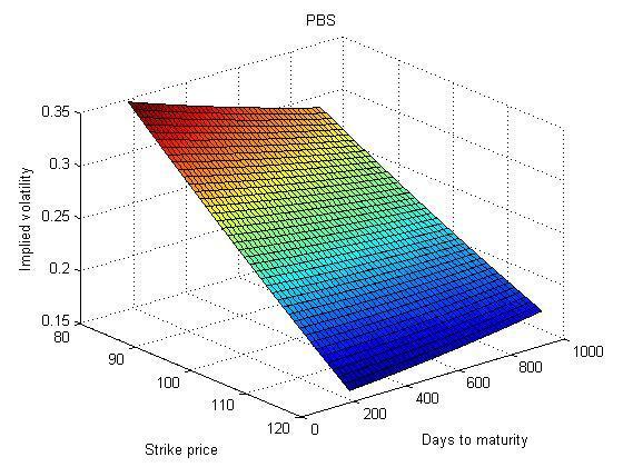
65 63