ReservePrism Simulation

Transcription

1 ReservePrism Simulation For Actuarial Loss Reserving and Pricing This document This document is made from ReservePrism Version

2 Table of Contents Preface... 4 Reserve Prism Simulation Models... 5 Planning Model... 5 Reserving Model... 5 Synthetic Claims vs. Real Claims... 6 What are Synthetic Claims?... 6 An IBNER Claim and Transaction Example... 6 What Can We Achieve from ReservePrism Simulation?... 9 True Stochastic... 9 Test existing method... 9 ReservePrism Stochastic Concepts ReservePrism Workflow ReservePrism R Architecture ReservePrism Structures and Parameters Simulation Project Overall Properties Accident Dates Range Random Seed Covariate Frequency Copula Correlation Annual Frequency Properties (Line Level) Annual Frequency, Trend, Exposure, Seasonality Occurrence to Claim Report Lag, Settlement Lag, and Valuation Frequency (Type Level) Severity Properties (Type Level) Size of Loss or Size of Each Payment Distribution Limit and Deductible P(0) Trend and Alpha Case Reserving Properties (Type Level) ReservePrism Simulating Example, A Claim s Life How ReservePrism Fits Data Claim Data Fitting Report Lag Fitting Annual Frequency Fitting Identify IBNR Claims Payment Lag or Settlement Lag Fitting

3 Heterogeneous Distribution Fitting Size of Loss Fitting, Survival Model Size of Loss and Payment Lag Copula Fitting Case Reserve Fitting on Outstanding Claims (IBNER) Triangle Fitting Use Report Count Triangle to Fit Annual Frequency and Report Lag Use Report Count and Close Count Triangle to Fit Settlement Lag Distribution Probability Fitting Brute Force Simulation Fitting Paid Loss Triangle (Brute Force) Fitting How to use ReservePrism Option 1: Prepare and Import Claim Transaction Data Example 1, Aggregated Data Example 2, Detail Transaction Level Data Import claim file Option 2: Prepare and Import Raw Triangle Data Triangle Sample in CSV format Import Triangle Data Run Simulations (once parameters are re-fit) Simulation Result Presentation Single Iteration Result Presentation In Planning Mode In Reserving Mode Rectangles Ultimate Loss, Ultimate Payment, and Reserves Confidence Intervals Presentation (from All Iterations) Confidence Level on Reserves, Ultimate Loss, Ultimate Payments Confidence Level on Ultimate Loss by Accident Years (Ultimate Summary Based) Rectangle Confidence Interval Appendix A - ReservePrism Tools and Utilities Distribution Tools Simple Distribution and Random Number Generator Mixture Distribution and Sampling Heterogeneous Distribution and Sampling Copula (Multivariate Distribution) and Sampling Distribution Fitting Tools Distribution Fitting Tool Copula Fitting Tool Mixture Distribution Fit

4 Convenient Stochastic Utilities Stage Bootstrapping LDF Curve Fitting Appendix B - Statistical Distribution References Beta Exponential Gamma Gaussian (Normal) Geometric Lognormal NegativeBinomial Pareto Poisson Weibull Apendix C - An Example to verify Traditional LDF Method

5 Preface ReservePrism is an enterprise actuarial platform useful for stochastic loss reserving, pricing, and planning. ReservePrism analyzes, parameterizes, and fits your claim data into its advanced R simulation engine. By simulating synthetic data that have similar statistical characteristics (e.g. lags, payments, frequency, case reserves, adjustment, etc), ReservePrism produces IBNR claims, develops the Outstanding claims, and combines the existing Closed claims, which will finally yield confidence interval of ultimate losses and reserves. To understand much of this documentation requires knowledge of actuarial science found in the Casualty Actuarial Society s syllabus of examinations. Standard actuarial and statistical terminology is not necessarily explained. We use statements from the statistical language R in this documentation. This is the source language for the models. ReservePrism uses the theory of probability and statistics, but is not entirely an exercise in these disciplines. Many of the algorithms use common sense to generate their results. The Casualty Actuarial Society developed a public loss simulation model. ReservePrism does much more than the public model. We have tried to make ReservePrism consistent with the public model to the extent possible. 4

6 Reserve Prism Simulation Models ReservePrism has two simulation models: Planning Model and Reserving Model. Planning Model The Planning Model generates synthetic claims for accident years you specify. You do not need to input actual claim data for this model. You may use actual claim data to determine the model parameters or you can select the parameters based on your knowledge. Using this model, you can generate pure synthetic claims for planning, testing, research, advanced modeling, and education purposes. The model can determine the majority of the parameters using raw triangles that you provide. Reserving Model Please use the Reserving Model for actual reserving analysis. For this model, you input real claim data (typically this is claim data up though a valuation date) to fit back all stochastic properties. Then, ReservePrism will generate Synthetic "pure IBNR" claims (Incurred but Not Reported claims), and develops them until closed. ReservePrism develops the actual Case Outstanding claims until closing stage by simulating their future transactions. This determines the "IBNER" reserve, another name for the "development on case reserves". 5

7 ReservePrism simply uses existing Closed claims to help calculate ultimate loss and ultimate payment rectangles. Synthetic Claims vs. Real Claims What are Synthetic Claims? Synthetic Claims are machine-generated insurance claims using the parameters that the user specifies. One purpose of ReservePrism is to enable the user to produce synthetic claims that have the same important statistical characteristics with regard to Annual Frequency, Loss Severity, Report Lags, Settlement Lags, Case Reserves Transactions, Adjustments, Payment Ratios, etc. An IBNER Claim and Transaction Example The Reserving Model completes the development on real claims outstanding as of a valuation date. This is more complicated than generating a synthetic claim. For each case outstanding claim, the model first generates a synthetic claim whose settlement lag is at least as great as the difference between the valuation date and the actual claim's report date. The model then generates future transactions on the open claim using the synthetic claim's transactions as a pattern. The following example illustrates this procedure. Below we use one actual outstanding claim (blue section) to depict how ReservePrism generates possible synthetic claim transactions (yellow section) and then combines them together to fulfill the IBNER development. Please note that these synthetic transactions are only one of possible future developments from this real claim, following the same stochastic 6

8 properties as other claims (and this claim as well), like payment distribution, settlement distribution, and payment count distribution, etc. In this example: Evaluation Date is 12/31/2014, and the claim s Report Date is 10/11/2013. The column "Case Reserve" is the change in the case reserve. This algorithm is one of the common sense algorithms mentioned in the preface. We are merging historical claim transactions and information from the simulated claim to create a complete set of transactions 1 for the IBNER claim. 1 Transaction Code in the sample Excel sheet next page: RPT - Reporting; EVA Evaluation Date; RES - Case Reserve; PMT Payment; INT40, INT70, and INT90 (System Generated) Interpolation Dates 7

9 Simulation No Occurrence Claim Transaction No No Date Action CaseReserve Payment /11/2013 RPT /11/ /23/ /24/ /13/ /13/ /19/ /20/ /5/ /5/ /5/ /6/ /6/ /6/ /31/2014 EVA /31/2014 RES /11/2015 PMT /31/2015 RES /5/2015 INT /18/2015 PMT /30/2015 RES /30/2015 RES /31/2015 RES /31/2016 RES /12/2016 PMT /16/2016 INT /30/2016 RES /2/2016 PMT /30/2016 RES /31/2016 RES /25/2017 PMT /12/2017 INT /31/2017 RES /13/2017 PMT /27/2017 PMT Hai You: Blue section are existing real claim transactions, the simulationno, Occ No, and Claim No columns are added for grouping purpose only Hai You: Following the EVA are simulated future transactions. Valuations Dates are simulated at each quarter end. EVA is added for marking purpose. Hai You: INT40, INT70, and INT90 are system generated interpolation dates, Claim closes at last payment date of 06/27/2017 8

10 What Can We Achieve from ReservePrism Simulation? Help to understand the life cycle of claims Build up true stochastic foundation of modern analytical loss reserving/pricing Develop alternative to traditional Triangle Methods Test your existing method True Stochastic Knowing that simple averages and abstract models are hard to satisfy, actuaries have been struggling on finding true stochastic way to help their predictions. Most of the time, the truth passes by unnoticed. We believe true actuarial stochastic lies beneath the claims, and can be explored well through the revolutionary modern computing technology. For data observations in a triangular display to support the actuarial prediction of alternative future realities, creativity is required. Daniel Murphy For example, people think Bootstrap Method is true stochastic, but let s examine it: 1. Residual= (A-E)/E.5, where A = Actual Incremental Paid Loss E = Developed Incremental Paid triangle, after applying all year weighted average LDF on accumulated Paid Loss (So here is ChainLadder1!!) 2. After resampling Residual triangle (This is the trend-lost part, assuming residuals are under uniform distribution, but why?), we will get R ; then get back the Pseudo incremental triangle A =E+ R * E.5 3. Then do another round of LDF development on A, using imaginary all year weighted average LDF from A, to get the ultimate loss (So this is the ChainLadder2!!) 4. Repeat step 2 and 3 for thousands of times, to get the ultimate loss confidence level. 5. Of course you can go to stage 2 bootstrapping, a gamma sampling process on each cell to compensate the model error of trend-lost effect, in step 2. Are you confident enough? Test existing method Please see Appendix C, page 94, An Example to verify Traditional LDF Method. In the following chapters, we will illustrate ReservePrism important concepts, how ReservePrism fits your data, and how ReservePrism produces ranges of output to guide and maybe test your current methods. 9

11 ReservePrism Stochastic Concepts ReservePrism Workflow ReservePrism R Architecture ReservePrism is pure R, very fast, and has advanced Windows front-end GUI. We have developed our advanced ReservePrism R Bridge to communicate in between. All data is saved and managed by the ReservePrism Database. ReservePrism R Architecture Data Import Dummy Windows User Interface ReservePrism Database ReservePrism R Bridge Result ReservePrism R Simulation Engine ReservePrism R Fitting Engine ReservePrism R Core Libraries Public Common R Libraries 10

12 ReservePrism Structures and Parameters A simulation project is one where modeler enters properties for line of businesses and types and initializes the simulation. A typical project can contain multiple lines of business (LOB), with each line of business consisting of one or more types of claims. The Line object will mostly define Annual Frequency properties. The Type object defined in the ReservePrism can be used to define coverage for a line. It will contain most of the required coverage properties such as payment pattern, lags, severity, case reserve activities, and recovery adjustment properties. A tree structure is the best way to describe the relationships among them, as shown below. If you run simulations for the project, ReservePrism will save the synthetic results into database, and present all kinds of confidence interval statistical analysis in separate tree structures attached to the project. 11

13 Simulation Project Overall Properties Accident Dates Range The earliest and latest Accident Dates play key important role in entire simulation 1. If either Claim Data or Triangle data is provided, these two parameters will be fitted first. For example, when a yearly Accident Year Report Count Triangle is provided, the system will detect your triangle accident year rows and set these parameters. 2. Usually, the earliest accident date is set at a year-starting date and latest accident date is set at year-end date. These two dates will determine how many accident year rows the resulting rectangle will have 3. VERY INTERESTING FEATURE: For example, in above project, original accident date ranges are fitted between 1996 and 2010 from real claim data. In Reserving Model, besides IBNR and IBNER development, suppose you are also interested in projecting claims for two future accident years (Planning Concept). You can change the Latest Accident Date to 12/31/2012, and the Annual Frequency parameter at line level will look like the following: 12

14 KEEP YOUR ORIGINAL EVALUATION DATE OF 12/31/2010, and run simulation. Following is a simulated Accident Year Count rectangle. The orange section is the projection for 2011 and 2012, assuming you assign annual frequency as Poisson Lambda 1200 each. Those claims will be reported in the same pattern as existing or IBNR claims (same Report Lag, of course you can change). 13

15 Thus, you did a combined simulation of Reserving Mode and Planning Mode Random Seed Random Seed is a number used to initialize a pseudorandom number generator. The choice of a good random seed is crucial in the field of computer security. However, in our case it is mainly used for testing the simulated result. By fixing the seed, we ensure that users can generate the same result with the same seed number when the simulation is run under the same assumptions. Please note that the simulation results are still truly randomly generated. Covariate The Covariate parameter adds another characteristic besides Line and Type. In regression analysis we also use the term independent variable to mean a covariate. In the simulation model, think of a covariate as another field in the simulated claim record. Covariate structure: Assume a covariate has m distinct values corresponding to index j, where j =1, 2, m. We will call the covariate "State", but it can be given any name. Then for each affected distribution, we will specify which parameter varies by State. This has to be defined for each type of distribution. For example, I set 2 lines, Auto and Home, and each line has one Type. I created a covariate called State to reflect my company s location: WI, IL and CA. From my experience, I can set the following proportions for each distribution. 14

16 How do we interpret above ratios? For occurrence (frequency), if there are m states indexed from 1 to m, set the parameters by state as p 1, p 2, p m. (In our example, p 1 =2, p 2 =1, and p 3 =2 respectively for WI, IL, and CA for Auto Occurrence). First let us draw the occurrences as the model currently does without covariates. Then, if n is the number of occurrences, the number by state is multinomial with parameters (n, p 1, p 2, p m ). In R, you would draw the number of occurrences according to the Poisson distribution. Then if n is the resultant number of claims, you would draw the vector of occurrences by state using rmultinom(1, size = n, prob = c(p 1, p 2, p m ) ). Notice that the probabilities do not need to add to 1 since the rmultinom function normalizes them so they add to 1. For Severity, the covariate parameter varies by distribution. For example, for lognormal distribution, let the "meanlog" parameter of the distribution vary by State. Suppose your Auto/PD Size of Loss distribution is lognormal(meanlog=8, sdlog=0.5), then after applying the covariate proportion of 3, 10, 5, for WI, IL, and CA respectively in our example, WI loss will be lognormal(meanlog=8*(3/18), sdlog=0.5), IL loss will be lognormal(meanlog=8*(10/18), sdlog=0.5), and CA loss will be lognormal(meanlog=8*(5/18), sdlog=0.5). For limit and Deductible, we directly apply the normalized ratio to dollar amount generated by Limit/Deductible distribution. 15

17 Frequency Copula Correlation When you have multiple Lines defined under the project, this Copula parameter can help to ensure the proper monthly occurrences correlation between Lines. For more technical details, please visit the Annual Frequency section right below on how to generate monthly occurrence, and in Copula Sampling section from Appendix A to see how Copula works. Annual Frequency Properties (Line Level) Annual Frequency, Trend, Exposure, Seasonality Annual Frequency, a discrete distribution, is defined at the Line level, as an "accident" or "occurrence" frequency. The system converts the annual frequency to monthly frequency during simulation. Following is an example of how synthetic claims are born: 1. In above picture, we set Annual Frequency as Poisson (lambda=4800) for year 2000, and let us focus on how claims are generated in July, Monthly Exposure is defined as <2,1,1,2,1,1,2,1,1,2,1,1>. 16

18 Monthly exposure for a year is normalized so that it sums to 1.0. In this example, this is equivalent to dividing the sum by 16. We obtain the vector: <2/16,1/16,1/16,2/16,1/16,1/16,2/16,1/16,1/16,2/16,1/16,1/16> 3. Seasonality will be normalized during calculation. For example, let us define the monthly seasonality as <5,1,1,1,1,1,1,1,1,1,5,5>. The example assumes that most accidents happened during the snow months November, December and January. Monthly seasonality for a year is normalized so that it sums to Since the total of the vector elements above is 24, the normalizing process would divide each element by 24/12= 2.0. Thus we have a final seasonality vector: <2.5, 0.5, 0.5, 0.5, 0.5, 0.5, 0.5, 0.5, 0.5, 0.5, 2.5, 2.5> SEASONALITY CONFIGURATION FOR CAT MODEL: Suppose Aug is hurricane season, and one hurricane can usually generate around claims. We can model this situation simply as follows: define the seasonality as <0,0,0,0,0,0,0,1,0,0,0,0>, set the annual frequency of year 2001 to Poisson (lambda=1), and set the Occurrence to Claim ratio to Trend factor is defined monthly, and will be accumulated as: CumulTrend (j) = CumulTrend (j 1) * TrendInput (j). In another words, to obtain 8% effective annual trend for year 2000, one would enter the amount 1.08 ^ (1/12) = for the monthly trend factor. Then trend factors accumulated for the year 2000, when applied, are actually, < , , , , , , , , , , , > 5. Now let us determine the Monthly Frequency parameter, using July 2000 as an example. In steps 2, 3, and 4 above we calculated vectors of exposure, seasonality, and cumulative frequency trend by month for the year We will use the 7 th element of each vector since July is the 7 th month. Recall that we specified the "base" annual frequency for the model as Poisson with mean lambda=4800. The Poisson parameter for the monthly frequency for July 2000 is calculated as: Poisson Lambda for July =Base Annual Frequency Lambda * Monthly Exposure for July * Seasonality Factor for July * Accumulated Trend Factor for July = 4800 * 2/16 * 0.5 * =

19 The actual number of claims is then simulated: rpois(1, )=346 2 Conclusion: in 07/2000, we will have 346 occurrences, and their Accident Dates are uniformly distributed in 07/ Important actuarial notes on trend and other frequency parameters: The trend factors are applied starting with the first month of the accident period for the model (January 2000 in the example above). Therefore, you might think of the "base" annual frequency input to the model as the level applicable for the month December 1999 in this case. The monthly exposure vector represents the relative earned exposure level by month. It does not represent the written exposure by month. Because the frequency parameter for each month is the product of the "base" annual frequency and the various other frequency parameters, the implication is that the seasonality and exposure factors are independent. For some purposes, it may be easier to just have one set of factors to represent the combined effect of seasonality and earned exposure distribution. Occurrence to Claim The Claim/Acc parameters determine how many claims of each type will be generated. The following table shows that an occurrence has a 2/3 probability of generating 1 BI and 1 PD claim, and a 1/3 chance of generating 1 PD claim. The actual number of claims of each Type arising from an occurrence is modeled via a multinomial distribution. In our example, we have two Types, PD and BI. 2 In this statement, "346" is the result of a sample of one from the Poisson(lambda= ) distribution. 18

20 Sample above proportion, rmultinom(1, 346, c(2, 1)) ( 229,117 Conclusion: in 07/2000, among 346 occurrences, 229 of them will produce 229 PD claims and 229 BI claims with the same Accident Dates respectively (since every pair of the claims are from the same occurrence); and 117 BI claims arise from the other 117 occurrences. Report Lag, Settlement Lag, and Valuation Frequency (Type Level) Report Lag is the number of days between claim s accident date and report date. Payment lag is the lag from report date to payment date or between consecutive payment dates (for multiple payments). For single payment claim, the payment date is also the claim close date. Case Reserve valuation is carried monthly, quarterly, or yearly. 19

21 Severity Properties (Type Level) Size of Loss or Size of Each Payment Distribution For single payment coverage, the system treats this parameter as distribution of entire loss. For multiple payments, the total loss is a compound distribution, and the system treats this parameter as the distribution of each payment. In either case, you do not have the ground-up loss dollar amount, but only the payment information under the policy. The System will fit this distribution by applying Survival Model. Reinsurance is not in the basic model at this time. Please consult us on the reinsurance topic. Limit and Deductible In ReservePrism, Limit and Deductible are defined by multinomial distributions. For example, in the following Limit and Deductible property for a Property Damage Type, 20

22 We can expect that claims (simulated) for this PD Type will have 33.3% chance to have Deductible of $1000, and 66.6% chance having Deductible of $2000. Then the Limit distribution for Deductible item of $1000 is defined as, Basically, this is another multinomial distribution. Which means, any claim that has $1000 Deductible, will have 50% chances to have Limit of $1,000,000, and 50% chances to have Limit of $2,000,000. From this calculation, we can say, there are about 16.67% of the claims will have limit of $1,000,000 and deductible of $1,000; 33.3% of the claims will have limit of $2,000,000 and deductible of $1,000. Another important concept involved here is how to apply Limit and Deductible to an individual claim to get final payments. To get payments, we will first cap the loss by Limit, and then apply Deductible. For example, with limit=$4500 and deductible=$500, if the claim has incremental losses $1000, $0, $2000, $3000, and $4000 during five periods, the policy payments we generate will be $500, $0, $2000, $1500, and $0 respectively, after applying Limit and Deductible. Yet for SIR, we will apply SIR dollar amount first to losses, and then cap the final payments to Limit. P(0) P(0) is the (uniform) probability of claim closure without payment at payment date, for reasons other than failure to exceed the deductible. In another word, it is simply the claim turn down ratio. Trend and Alpha 21

23 Severity Trend is the change in mean loss size for newly incurred losses, considering cost per claim, inflation, etc, accumulated across accident years. The alpha [0,1] allows you adjust the trend along accident years, development years, and calendar years. For example, if monthly trend is set to at starting year of 2000, system will visualize the accumulated trend across accident years. The alpha 3 intelligently adjusted the accumulated trend factor between accident date and payment date, thus achieving the trending along accident years, development years and calendar years. System will provide a unit triangle, which assumes the loss from starting accident year and starting development age is 1, to illustrate the overall influence to the severity by the cumulative trend and alpha combined. Let us look at 3 examples with alpha set to 0, 0.5, and 1.0 respectively. 3 Butsic s alpha parameter was originally defined in Robert Butsic s paper on The Effect of Inflation on Losses and Premiums for Property-Liability Insurers, Casualty Actuarial Society Discussion Paper Program, 1981, pp

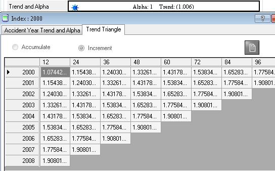
24 23

25 Case Reserving Properties (Type Level) Each insurer has a philosophy on how it sets and adjusts its Case Reserves between the report date and closing date of a claim. The Case Reserving Properties parameters enable the modeler to determine an adjustment procedure to apply to the simulated claims. To understand this, first rescale time so that time 0 is the report date and time 1.0 is the closing date. For example, time 0.40 is a time 40% of the way between the report date and the closing date. The System calculates case reserve adequacy factors sampled from distributions at four interpolating times: 0, 40%, 70, and 90%. The 100% point will always have factor 1.0, so there is no distribution needed. In the single payment model, if the loss is above the defined Threshold, system will also apply the Estimated P(0) ratio, to reflect the claim adjuster s estimation of P(0). Let us use an Excel example to see how Case Reserves are generated. o The four Adequacy distributions are defined by you from your experience. In the example, we set the sdlog to 0 so that random sampling always yields the mean value of the case reserve adequacy meanlog meanlog meanlog meanlog sdlog0 0 sdlog40 0 sdlog70 0 sdlog90 0 mean factor.. o o This is a single payment example with loss at $35,673. It is sampled from a lognormal (meanlog=10, sdlog=0.8) Size of Loss distribution, policy Limit is $1,000,000, deductible is $5000. So the Single Payment is $30,673. P(0) is defined as 0.4. System will do a random sampling to decide if the real payment is 0 or the $30,673 above. In our example, 1-runif(1)= > 0.4. So we have payment of $30,673, as shown in Cell(C, 22) 24

26 o o o o Threshold is defined as $100, which is less than the loss, so we will apply Est P(0), 0.4, as shown in column E with formula (1-Est P(0) ) * CaseReserve. Thus column E is the needed case reserve if the loss is paid times the estimated probability that the claim will be paid. Please be note Column F, where Incurred Loss = Case Reserve (Column E) * factor (Column B) + Cumulative Paid (Column C) at 0, 40%, 70% 90% and 100% points. Incurred Losses at other times use linear interpolation of the Incurred Loss determined at these five points. What is Column A? It is the rescaled time described above. For example, the claim report date is 03/10/2000 and payment date is 08/15/2002, when $30,673 is paid. Then the Payment Lag =08/15/ /10/2000 = 888 days. Cell(A2) represents the report date where valuation lag is 0; Cell(A3) represents a date of 888* /10/2000, which is 04/23/2000. This example does not yet reflect the system design that valuations are generated at monthly, quarterly, or yearly intervals. Instead, this example focuses on the case reserving concept. Column I is the final Case Reserve Transactions output. This method of generating case reserve changes is not intended to be a behavioral model of the claim adjusting process. It is designed to reflect the fact that case reserves cannot be set at the ultimately needed value, since the ultimate value is not known until the claim is closed. This process is also discussed in the documentation of the public Loss Simulation Model. 25

27 26

28 ReservePrism Simulating Example, A Claim s Life Following the previous chapters, let us combine the Frequency, Severity, and Case Reserving concepts together, to see how a synthetic claim is generated, developed, and closed. Then in later chapter, once real claims or triangle data are introduced, we can apply the same concept to develop IBNR and IBNER claims with real properties from real claims. Simulation Mode: Planning Mode, pure simulation. Simulation Accident Year Range: LOB: Commercial Auto, Type: BI Covariate: None Commercial Auto LOB Frequency Properties: Annual Frequency: Poisson, lambda=4800, for accident year 2000~2009 (before trend) Monthly Exposure: 2,1,1,2,1,1,2,1,1,2,1,1, for year 2000, all 1 for rest of the years Monthly Trend: , starting from 01/2000 Seasonality: 5,1,1,1,1,1,1,1,1,1,5,5, same for years 2000~2009 Occurrence to Claim: 100% to BI Type, with only BI Type exists under Commercial Auto LOB. Let us first focus on Accident Year 2000: Exposure Pro Rata vector:: <2/16,1/16,1/16,2/16,1/16,1/16,2/16,1/16,1/16,2/16,1/16,1/16> Seasonality Normalized vector: <2.5, 0.5, 0.5, 0.5, 0.5, 0.5, 0.5, 0.5, 0.5, 0.5, 2.5, 2.5> Accumulated Trend vector: < , , , , , , , , , , , > Monthly Frequency: Poisson with the following means: Lambda= 4800 * 2/16 * 2.5 * =1509 (Jan 2000); Lambda= 4800 * 2/16 * 0.5 * =314 (July 2000);. = 4800 * 1/16 * 0.5 * =152(Feb 2000); Sample from Monthly Frequency: rpois(12, c(1509, 152, 153, 308, 155, 156, 314,158, 159, 320, 805, 810)) Occurrences Generated for Accident Year 2000: BI Accidents Generated for Accident Year 2000: Do similar calculations for 2001 to 2009; these will be total accidents simulated for each year: Then let us switch back and focus on July, 2000: Among the 301 BI accidents, there is one claim with accident date: 07/23/2000, let us mark it ClaimNo=XX and let us examine this claim s whole life. 07/01/ as.integer(runif(1, 0, 30))= " " 27

29 ClaimNo AccidentDate Line Type XX 07/23/2000 Commercial Auto BI BI Type Lag Properties: Payment: Single Payment Report Lag Distribution: Exponential (rate= ), mean around 90 days Payment Lag Distribution: Exponential (rate= ), mean around 365 days Adjustment Lag Distribution: None (no re-opened claims) Sample from report lag to get Report Date= Accident Date + Report Lag in Days 07/23/ as.integer(rexp(1,rate= ))= Sample from Payment Lag to get Payment Date= Report Date + Payment Lag in Days 11/29/ as.integer(rexp(1,rate= ))= Since this is a Single Payment claim, it will be closed at 04/07/2001 also. ClaimNo AccidentDate ReportDate PaymentDate CloseDate Line Type XX 07/23/ /29/ /07/ /07/2001 Commercial Auto BI BI Type Severity Properties: Size of Loss Lognormal (meanlog= , sdlog= ) Distribution: Mean about $100,000 and Sd about $100,000 P(0): 0.2, means about 20% claims will be rejected by adjuster Severity Trend: monthly, starting on 01/2000 Butsic Alpha: 0.5 Deductible: $2000, proportion 2 Limit: $100,000 Deductible: $1000, proportion 1 Limit: $100,000, proportion 1 Limit: $200,000, proportion 1 Sample from uniform distribution and compare with P(0) to see if this claim needs payment: runif(1, 0, 1)= >0.2, unfortunately, need to pay this claim Sample from Size of Loss distribution to get loss dollar at accident date: rlnorm(1, meanlog= , sdlog= )= $ Apply trend and Alpha from Accident Date to Payment Date: 28

30 trend <- cum_trend_accident * ((cum_trend_payment /cum_ trend_accident) ^ alpha) = * ( / )^0.5 = Actual Loss dollar = Loss * trend= $ * =$ Among the total claims, limit and deductible for each claim are calculated as Step 1: rmultinom(1, 71193, c(2,1))= claims will have deductible of $2000 and claims have deductible $1000 Step 2: The claims with deductible $2000 all have limit of $100,000 Step 3: rmultinom(1, 23571, c(1,1))= Among the claims with deductible $1000, claims will have limit of $100,000 and claims have limit of $200,000 Our ClaimNo XX, whose total "ground up" loss is $65,879.32, happens to have Limit of $100,000 and deductible of $2000, so the final payment equals $63, after applying the deductible. Claim Accident Report Payment Close Line Type Limit Ded Loss Payment No Date Date Date Date XX 07/23/ /29/ /07/ /07/2001 CA BI $ $ Now let us examine Case Reserve Transactions for our Claim XX: BI Type Case Reserve Properties: Valuation Frequency: Monthly Est P(0): 0.4 Threshold: $300, actual loss $ is above the Threshold, so, apply Est P(0) Fast Track: $0, means, there is no fast track case reserves applied to claims 0% Case Reserve Adequacy: Lognormal(meanlog= , sdlog=0), mean % Case Reserve Adequacy: Lognormal(meanlog= , sdlog=0), mean % Case Reserve Adequacy: Lognormal(meanlog= , sdlog=0), mean % Case Reserve Adequacy: Lognormal(meanlog= , sdlog=0), mean Let us first lay out the valuation dates, payment date, and interpolation dates. There will be case reserve transactions generated at these dates. Incurred Loss will be interpolated between interpolation dates. Please see the following Excel calculation to see how to get all detail transactions. 29

31 Total payment lag T= =129 (days) 0.40 date INT40: 0.4 * = " " 0.70 date INT70: 0.7 * = " date INT90: 0.9 * = " " (report date, also INT 0) (valuation date 1, first month end) (valuation date 2) (INT 40) (valuation date 3) (INT 70) (valuation date 4) (INT 90) (valuation date 5) (payment date, also, claim close date) And this concludes (Claim XX) one synthetic claim s life with entire Transactions. Claim No Transaction Date Action Case Reserve Payment XX 07/23/2000 ACT 11/29/2000 REP 35,586 11/30/2000 RES 61 12/31/2000 RES 1,890 01/19/2001 INT40 1,158 01/31/2001 RES /27/2001 INT70-1,047 30

32 02/28/2001 RES 37 03/25/2001 INT /31/2001 RES 11,881 04/07/2001 PMT -50,018 63,879 31

33 How ReservePrism Fits Data Fitting Claim or Triangle Data is the foundation of Synthetic Claim Simulation in the Reserving Model.. The fitting process exposes your critical claim data properties, and more importantly, helps determine parameters for the later simulation process. STATISTICAL PHILOSOPHY 4 : CAN WE ENVISION FUTURE FROM HISTORY? For example, you have fitted and visualized the settlement lag distribution from your existing claims, but is your claim settlement pattern going to change in next quarter or next year? This assumption will affect the development of IBNR and Case Outstanding claims. We cannot answer this question. However, ReservePrism sets up a comprehensive and flexible platform on which you can either assume the future will follow the same historical pattern, or you can change the distribution property for future to reflect your vision and opinion. STATISTICAL PHILOSOPHY ON OPTIMIZATION OR FITTING (SUCH AS CURVE FITTING OR DISTRIBUTION FITTING): DOES THE OPTIMIZED THING REPRESENT THE TRUE THING? If you have claim data or triangle data imported (please see later chapter), you will see that most of the parameters in your project have STAR buttons. They are fitted by default or to be fitted parameters. WE STRONGLY RECOMMEND THAT YOU RE-FIT ALL OF THE PARAMETERS BEFORE SIMULATION. Simply click the star button to open the fitting window to fit the parameter. Once you accept the fitting result, the button on left will also be refreshed. At any time, you still can manually change the parameter value by clicking the button on left, ignoring the fitted values. Sample: Parameters that are fitted and can be fitted have a yellow star button on right side. Claim Data Fitting 4 A Statistical Philosophical question cannot be easily answered. It needs wisdom to accept. For example, is life determined? Or is life Stochastic? 32

34 In statistics, a probability distribution assigns a probability to each measurable subset of the possible outcomes of a random experiment. Insurance Claim data contains the richest stochastic information, such as Annual Frequency 5, Report Lag, Settlement Lag, Size of Loss (or Size of Each Payment), Limit and Deductible, Payment Patterns, and Case Reserving for IBNER, etc. ReservePrism will fit most of these important features in order to draw the whole picture of the complicated insurance claims. Report Lag Fitting Report Lag = Report Date Accident Date, as seen from the sample observation graph below, it is under a distribution. In every fitting window, the first tab tells you the fitting observation filtered by Type and Line; second tab shows its Empirical Graphs. 5 Frequency here means number of claims per time unit, not the number of claims per exposure unit. Reserve Prism does not use exposure or premium data. 33

35 In above window, I choose Homogeneous 6 Weibull distribution family to start the Report Lag fitting. Homogeneous means that the Weibull parameters do not vary by accident 6 Homogenous comes from the Greek for "same kind".in ReservePrism, Homogeneity represents the same category or distribution within the whole population. Its opposite is Heterogeneous Distribution, which means a population contains different distributions across years. Yet, a Mixture distribution is a combined distribution among population, without any time constraint. Markov Chain is also a mixture distribution, but its marginal stages are changing with certain switching probabilities. 34

36 period. The System will then fit back parameters automatically. Is it a good fit? QQ-Plot looks pretty well, but the KS Test has P-Value=0, and from the observation graph, you can see a little lump in Histogram or Density. Could it because Report Lag has been changed after certain accident year? Let us keep playing with this sample in the later Heterogeneous Distribution Fitting section. Annual Frequency Fitting Annual Frequency is automatically fitted every time Report Lag parameter is changed (either through re-fit or from a direct modification by user). System will show you the fitted Annual Frequency by accident years. How to obtain Annual Frequency from a Claim file? It is the procedure to obtain the ultimate claim count for each accident year. 1. Get each Accident Years real claim count C 2. Find the Report Lag distribution L, by fitting from the claims Report Date and Accident Date, as stated in previous section 3. Calculate the Integrated Probability P for distribution L. by integrating the Density Function along accident years (you can also use mid-year Cumulative Density for a very simplified calculation). This P represents the claims reporting probabilities along accident years. 4. Annual Frequency, the ultimate claim count for each accident year, AF=C / P 35

37 From above fitted Annual Frequency graph, you can also see the approximate IBNR claim count for the most recent accident years, which is the difference between the white bar, the fitted annual frequency, and the dark bar, the real claim count. Identify IBNR Claims Incurred-But-Not-Reported Claims are one of the actuarial mysteries. The accidents happened before the Evaluation Date, but will be reported after the evaluation date and thus are currently unknown. In traditional deterministic loss analysis, or chain ladder methods, actuaries pick Loss Development Factor (LDF) from various averages, experiences, and special adjustments to guess the possible ultimate values and then deduct the accumulated values as of the evaluation date to get IBNR counts and dollar amounts. As indicated from above Annual Frequency Fitting section, ReservePrism figures out this actuarial mystery simply through stochastic fitting. In the later simulation stage, IBNR claim counts and their various dollar amounts will be presented through confidence intervals from simulation iterations Payment Lag or Settlement Lag Fitting Payment or Settlement Lag is the lag (in days) from report date to payment date (for single payment) and between consecutive payment dates (for multiple payments). # ClaimNo AccidentDate ReportDate PaymentDate CloseDate # 9 06/09/ /03/ /10/ /10/2013 # 10 12/10/ /03/ /01/2012 # 10 12/10/ /03/ /12/2012 # 10 12/10/ /03/ /11/2012 # 10 12/10/ /03/ /10/ /10/2013 ReservePrism s fitting engine will distinguish different payment patterns to get individual payment lag(s) for each claim. The rest of the fitting process will follow the same procedure as Report Lag Distribution Fitting. Heterogeneous Distribution Fitting If your business changed at certain year, for example, the claims were reported much faster after 2007 (perhaps due to policy changes, or maybe accidents became more severe), we can specify the report lag distribution as a Heterogeneous Distribution. The same true for the settlement lag. So let us continue the example from previous Report Lag Fitting section, but 36

38 this time, let us try Heterogeneous Fitting by changing the report lag distribution after 2007, but still assuming it is under Weibull distribution family. The following picture shows the interface of fitting Report Lag with Heterogeneous Distribution, where you can pick the accident years when the distribution changed, and change the distribution family on right side panel from that year. The fitting QQ Plot is not close enough to the 45-degree line in the head and tail part. I am still not satisfied with the result. So let me try a very useful implementation from above Heterogeneous Distribution interface. Let us investigate each accident year s Report Lag Distribution individually, still assuming they are all follow the Weibull distributions. 37

39 Instantly, you can see report lags from accident year 1996, 1997, 1998 to 2009, and 2010 have significantly different shape and scale parameters. Things definitely changed in those years. But my KS Test 7 still gives me a very small P-Value, could it because at certain year(s), the Report Lag is not under Weibull distribution? I can keep doing further research on this set of claim data. But can you see the powerful analytical platform ReservePrism provides? Size of Loss Fitting, Survival Model Insurance claim has only payment information available, with real loss dollar amount being censored and truncated by limit and deductible. System will fit Size of Loss (or Size of Each Payment) distribution with Survival Model using payment, limit, and deductible. 7 KS Test is pretty sensitive. 38

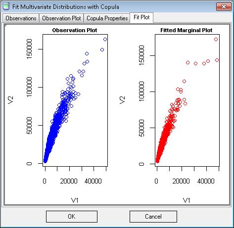
40 By optimizing the negative logarithm of the likelihood function (negloglike), the Survival Model back-fits the Claim Severity distribution, given claim Paid Amount, Limit and Deductible. Self-Insured Retention (SIR), and trend, if applied, can also be applied in our customized Survival Model. Here are the main points: ### when loss is over limit, we don't know the real loss, but we know limit is the capped loss X1=log(1-Probability(SizeOfLoss, limit / alpha_trend))) ### for normal payment, which we know loss = payment + deductible X2=Density(SizeOfLoss, (payment + deductible)/ alpha_trend, log=true) ### remove deductible truncated claims by subtracting log(1-fx(d)) X <- (X1+X2) - log(1-probability(sizeofloss, deductible/alpha_trend)) By optimizing (minimizing) the X, system will get the best fit Size of Loss distribution. Size of Loss and Payment Lag Copula Fitting Given a claim file, let us determine the correlation, if exists, between the Size of Loss and the Payment Lag. The following Copula Fitting window will pop up, showing the observation plot between the Loss Amount and Payment Lag. In this fitting, we filtered out claims with payment > limit and payment < deductible, because we don t know the real loss value from those claims. From the example plot, we cannot observe a clear correlation between Loss and Payment Lag. But let us still try to fit that Copula just as an illustration, 39

41 Click the Fit button, system will try to fit potential Copula correlation. But it confirms the hypothesis that there is no correlation in our example. Please visit Copula Fitting Tool in Appendix A, page 71, to see an existing correlation fit. If you are sure there is no correlation between Loss and Payment Lag, we recommend just uncheck the box to disable the Copula parameter to save significant simulation time. 40

42 Case Reserve Fitting on Outstanding Claims (IBNER) RESERVEPRISM PROVIDES AN INNOVATIVE APPROACH TO ESTIMATE THE FUTURE CLAIM DEVELOPMENT ON CASE RESERVES AND PAYMENTS (IBNER). Suppose we have already parameterized the model from the fitting process and we wish to use this model to develop a claim that is outstanding on the valuation date of the data (the "actual claim"). We assume that the data contains the accident date, report date, payments and case reserve history up to the valuation date. We will describe how to use the model to determine future reserve changes and payments in this chapter. The process described here is a practical common sense calculation. It is one way to complete the development on case outstanding claims. First, we can calculate s, the time between the valuation date and the report date. We then use the JM algorithm to determine t, the remaining time until settlement given that the settlement lag exceeds s. The settlement date then equals report date + s + t, and the settlement lag is equal to s + t. JM Generic Conditional Sampling Algorithm JM Algorithm refers to our generic conditional sampling algorithm authored by Joe Marker. The main point is, if I want to sample from any distribution, for example a normal (mean=10, sd=5) distribution, and I want the random number always bigger than 8, how? Please contact us for more algorithm detail. We can rescale time so that the report date is time 0 and the settlement date is time 1. Under this rescaling, the rescaled valuation date is d = s / (s+t). We then use the model to simulate claims until the settlement lag exceeds s. This last "simulated claim" contains the information we need to project future settlement on the actual claim. For the simulated claim, there are various case reserve changes and payments after its rescaled time d. We then use a multiple m of these amounts as the projected amounts for the actual claim. That is, if there is a payment x at rescaled time r > d for the simulated claim, then the actual claim will have a payment at rescaled time r equal to m times x, where: m = actual case reserve at time d simulated case reserve at time d 41

43 Let us use an example. Evaluation Date is: 12/31/2014. Assume your company is doing quarter-end valuations. You have already fit the claim transaction data and parameterized the model. Assume you have: Known Properties: Number of Payments: Geometric (prob= ), mean=6, sd 5 Payment Lag: Exponential (Rate= ), mean 75 days, dev 75 days. Valuation Frequency: Quarterly Size of each Payment: Lognormal(meanlog= , sdlog= ) mean $3,600 Limit and Deductible: $100,000 limit, no deductible Est P(0): 0 Threshold: $0, Fast Track: $0, Trend and Alpha: Ignore 0% Case Reserve Adequacy: Lognormal(meanlog= , sdlog=0), mean % Case Reserve Adequacy: Lognormal(meanlog= , sdlog=0), mean % Case Reserve Adequacy: Lognormal(meanlog= , sdlog=0), mean % Case Reserve Adequacy: Lognormal(meanlog= , sdlog=0), mean The following table lists one actual open claim s existing transactions. How will this actual Open claim develop with possible future Payments and Case Reserves? TransactionDate Action CaseReserve Payment 10/11/2013 RPT /11/2013 RES /23/2013 PMT /24/2013 RES /13/2013 PMT /13/2013 RES /19/2013 PMT /20/2013 RES /5/2014 PMT /5/2014 PMT /5/2014 PMT /6/2014 RES /6/2014 RES /6/2014 RES o Please read chapter ReservePrism Simulating Example, A Claim s Life on how ReservePrism does simulation. o For Open claim, let us start with sampling future number of payments, with JM Conditional Sampling Algorithm. There are 6 existing payments for this claim, then, 42

44 Future Number of Payments=conditionSample(Geometric (prob= ), existing=6) = 7 So, we know we will have 7 future payments. o Let us sample the 7 future payment dates. Since this claim is already reported, s, the time between the valuation date and the report date, is equal to 12/31/ /11/2013 = 446 days; Let us determine the first future payment date, which is equal to report date + s + t, where t is the remaining time until settlement given that the settlement lag exceeds s. t=conditionsample(exponential (Rate= ), minimumlag = s = 446)=46 days Payment Date 1 = 12/31/ =02/11/2015 For the rest of the 6 future payments, let us simply sample payment lag distribution to get their payment dates. Payment Date( i) = Payment Date (i-1) + sample(exponential (Rate= )), i=2,3,4,5,6,7 o Let us sample the 7 future payments, applying limit and deductible, trend and alpha, etc. Please note one important thing that, this claim has existing payments totaled $1, , the policy limit is $100,000, and deductible is 0. This means, limit and deductible are already applied by adjuster. Otherwise, we will have to apply remaining limit and deductible calculation from the future 7 payments. 7 Payments = Sample(Lognormal(meanlog= , sdlog= ), n=7) Till now, we have these unscaled payment transactions TransactionDate Action CaseReserve Payment 12/31/2014 EVA /11/2015 PMT /18/2015 PMT /12/2016 PMT /2/2016 PMT /25/2017 PMT /13/2017 PMT /27/2017 PMT o As previously discussed, we will generate the quarterly valuation dates, interpolation dates, and the (valuation lag) / (settlement lag) ratios as well. But we don t know the Case Reserve Transaction dollar amounts yet. Let us combine the existing (blue section), generated (white section), and unknown (orange section). 43

45 valuation lag/settlement lag Transaction Date Action Case Reserve Payment /11/2013 RPT /11/ /23/ /24/ /13/ /13/ /19/ /20/ /5/ /5/ /5/ /6/ /6/ /6/ /31/2014 RES /11/2015 PMT /31/2015 RES /5/2015 INT /18/2015 PMT /30/2015 RES /30/2015 RES /31/2015 RES /31/2016 RES /12/2016 PMT /16/2016 INT /30/2016 RES /2/2016 PMT /30/2016 RES /31/2016 RES /25/2017 PMT /12/2017 INT /31/2017 RES /13/2017 PMT /27/2017 PMT o How to generate future Case Reserve Transactions (orange section) and the scaled future payments? Since we already have all the simulated payments, dates, and ratios, let us keep simulating the Case Reserves by interpolation. But keep in mind that, we cannot change the existing transactions (blue section).. In this example, m = actual case reserve at time d =0.79 simulated case reserve at time d Orange section is the final rescaled Case Reserve Transactions. As a summary, this will be the entire claim history, with the orange section as its IBNER development. Please also see the Excel image for detail calculations. 44

46 TransactionDate Action CaseReserve Payment 10/11/2013 RPT /11/ /23/ /24/ /13/ /13/ /19/ /20/ /5/ /5/ /5/ /6/ /6/ /6/ /31/2014 EVA /31/2014 RES /11/2015 PMT /31/2015 RES /5/2015 INT /18/2015 PMT /30/2015 RES /30/2015 RES /31/2015 RES /31/2016 RES /12/2016 PMT /16/2016 INT /30/2016 RES /2/2016 PMT /30/2016 RES /31/2016 RES /25/2017 PMT /12/2017 INT /31/2017 RES /13/2017 PMT /27/2017 PMT

47 46

48 Triangle Fitting Development Triangles are currently widely used. The amount of information in a triangle is substantially less than is contained in detailed claim data. Therefore, modeling using a triangle requires many more assumptions than modeling using detailed data, and is much less accurate. The process described in this section is another process that we believe is a common sense, practical one. We do not claim that it is primarily statistical in nature. We describe the process so that the modeler can decide whether it is reasonable for his or her application. We do not believe that any procedure using only a development triangle gives an accurate projection of loss development. The unfortunate fact is that often only triangle data is available.,report Count Triangle maintains the relationship between overall claims happened during an accident year and how they are reported in the consecutive development years. Claim s detail accident dates and report dates are lost, with only year information kept. o Close Count Triangle (Close with Payment + Close without Payment) tells the story of how those reported claims in each development year close at consecutive calendar years. We lost the important information such as, how many payments happened to each claim until they close? When closed without payment, is the loss under deductible, or is claim simply rejected by adjuster? Of course, we only have year information. We don t really know the detail claim closure date. o Paid Loss Triangle maintains the accumulative payment for each calendar year from claims happened in certain accident year and reported after certain development years. We don t know which claims those payments belong to, we don t know whether or not those payments will close the claim, and we even lost the mean payment information. ReservePrism uses above triangles to fit required parameters and simulates only in Planning Mode. When fitting triangles, system implements Average Absolute Incremental Error (AAIE) concept to feed the optimization engine. AAIE can be used to determine how close two triangles are to each other. The smaller this number is, the closer these two triangles are. For example, in Report Count Triangle fitting, system uses assumed report lag distribution to generate a pseudo Report Count Triangle and compare the AAIE with the real Report Count Triangle. When the AAIE is optimized or minimized, the assumed Report Lag will be treated as real Report Lag. 47

49 Use Report Count Triangle to Fit Annual Frequency and Report Lag Reported Count Triangle contains hidden information such as Annual Frequency and Report Lag, but we need to use optimization algorithm to find the best values. 1. Let us call the actual Incremental Report Count Triangle R 2. Get each Accident Years real claim count C, which are row summary from R 3. Assume a Report Lag distribution L, and calculate the Integrated Probability Density P for distribution L along accident years. This represents the accident year probabilities for claims to be reported. 4. Annual Frequency, the ultimate claim count for each accident year, AF=C / P 5. Fitted Report Count Triangle R =C * p, where p is calculated from P as the cumulative probability at the appropriate state of development. You cannot simply use 48

50 Density Function of L, because the Density is a point to point value. We have to implement the integration with the best assumption that C claims uniformly arise from each accident year. 6. When minimizing the AAIE value of = R- R, distribution parameters for L are used as feeds. The optimization process will yield to the Report Lag distribution with the best fit parameters. Then perform step 3 and 4 one more time to get the optimized Annual Frequency AF. 7. (Optional) System also allows you to assume a Heterogeneous Report Lag distribution, and following the same logic above, fits out different Report Lag distributions from different accident year groups. This process is similar to optimizing Annual Frequency from claim file, with the only but critical exception that the Report Lag distribution is unknown. From claim file, we can directly fit the Report Lag distribution first as discussed in Claim Data Fitting, thus, more accurate and much faster. 49

51 Use Report Count and Close Count Triangle to Fit Settlement Lag ReservePrism uses both Report Count Triangle and Close Count Triangle to find possible Settlement Lag distribution. You will have to assume Number of Payment distribution for this coverage since it cannot be obtained from any triangles. We have developed two ways to fit the Settlement Lag. Let us use a very simplified example to illustrate this process. Incremental Report Count Triangle R and Closed Count Triangle C are known as shown, and assume we know each claim will be paid twice in average. Let us find out Settlement Lag distribution. 50

52 Mean Number of Payment for each claim: 2 Incremental Company Reported Claim Count Triangle R Acc Year Incremental Company Closed Count Triangle C Acc Year Distribution Probability Fitting o Assume a Payment Lag distribution L, o Form a bin along development years (in days), then divide it by number of payments. bin<-seq(from=365, to=40 * 365, by=365) bin<-bin/numberofpayments=bin/2 bin= o Calculate the Integrated Incremental Probability Density P for distribution L along the bin size. This P represents the calendar year probabilities for claims to be paid. For example, if P (1) = %, it means there is % possibility for a reported claim to be paid in 180 days, which in turn makes that claim close around 365 days. P<-Increment(Integrate(L, bin)) o Form a simulated Close Count Triangle C =C1+ C2 C1=P * 3 reported claims in cell (1993, 12), which will spread the 3 claims to be possibly closed along calendar year 12, 24, 36 C2=P * 2 reported claims in cell (1993, 24), which will spread the 2 claims to be possibly closed along calendar year 24, 36, 48 o Minimize the AAIE value of = C- C, using distribution parameters of L as optimization feeds. The optimization process will yield to the Payment Lag Distribution L. Brute Force Simulation Fitting 51

53 o Starting from the 3 claims from Report Count Triangle R cell (1993, 12), let us simulate their Report Dates from a uniform distribution. This assumes that they were reported randomly inside year Then do the same thing for the 2 claims in cell (1993, 24). Report Dates in 1993< as.integer(runif(3, 2, 365)) Report Dates in 1994< as.integer(runif(2, 2, 365)) o For each of the 5 reported claims, let us generate 2 payment lags from the assumed Payment Lag distribution L, till its close date. Payment Date 1 for Claim i<-report Date for Claim i + sample (L) Payment Date 2 (Close Date) for Claim i<- Payment Date 1 for Claim i + sample (L) i=1,2,..5 o Form a simulated Close Count Triangle C with the Close Dates (second payment dates) simulated for all the 5 claims. o Minimize the AAIE value of = C- C, using distribution parameters of L as optimization feeds. The optimization process will yield to the Payment Lag Distribution L. Paid Loss Triangle (Brute Force) Fitting Paid Loss Triangle has huge information loss when payments are simply aggregated by calendar years. ReservePrism implements Brute Force method to find Size of Loss distribution, using Incremental Paid Loss Triangle P, Incremental Report Count Triangle R, and Incremental Close Count Triangle C, Limit and Deductible (you define), Trend and Alpha (you define), P(0), Number of Payments (you define), and the fitted Payment Lag from previous section. The whole process basically performs claim simulation to form a simulated paid loss triangle, using all the known triangles and parameters. This process can take very long time and usually, the resulting AAIE is around 40% or 50% rough. o Fit Payment Lag PL o Roughly fit P(0) by P(0)=Sum(Incremental Close Without Payment Count)/Sum(C) o Generate each claim s report date by uniformly sampling in each development year. Claim Report Dates<-as.integer(runif(r, (age-1) * , age * 365)) R= each cell value from the Incremental Reported Count Triangle R o Generate each claim s payment date from sampling the PL by Number of Payment times. This will form a Closed Count Triangle C, but with the premise of the payment counts distribution. o Appling P (0) * C to simulate a Closed with Payment Count Triangle CP. 52

54 o Assume a Size of Loss distribution LOSS. o If there is Copula defined between LOSS and PL, system will then instead sample from the marginal distribution with Number of Payments, to get the lags and loss. o Form a simulated Paid Loss Triangle P by sampling LOSS inside CP, with the defined Number of Payments distribution, applying Limit and Deductible o Minimize the AAIE value of = P- P, using distribution parameters of LOSS as optimization feeds. The optimization process will yield to the Size of Loss Distribution LOSS. 53

55 How to use ReservePrism Option 1: Prepare and Import Claim Transaction Data SYSTEM ACCEPTS CSV FORMAT (COMMA SEPARATED TEXT FILE). REMOVE THE COMMA, SEPARATOR FROM MONEY VALUE TO AVOID CONFUSION. DATES NEED TO BE FORMATTED IN GLOBAL DATE FORMAT, SUCH AS THESE ARE MANDATED COLUMNS: CLAIMNO, ACCIDENTDATE, REPORTDATE, PAYMENTDATE, LINE, TYPE, LIMIT, DEDUCTIBLE, PAYMENT, CASERESERVE, CLAIMSTATUS SET DATA TO 0, IF MANDATED COLUMN IS MISSING. FOR INSTANCE, IF YOU DON T HAVE CASE RESERVE VALUE, MAKE THAT COLUMN ALL 0. SET LIMIT TO A BIG NUMBER, SUCH AS 1,000,000, IF THERE IS NO POLICY LIMIT INFORMATION PROVIDED. Example 1, Aggregated Data In many cases, only detailed claim amounts available for each claim are the cumulative amounts as of the evaluation date. In these cases, the system will use the Single Payment Model. 54

56 IN THIS CASE, THE CLAIM CLOSE DATE HAS TO BE TREATED AS PAYMENT DATE ClaimNo ReportDate Line Type AccidentDatePayment PaymentDatLimit Deductible ClaimLiabiStatus CaseReserve AUTO Liability TRUE CLOSED AUTO Liability TRUE CLOSED AUTO Liability TRUE CLOSED AUTO Liability TRUE CLOSED AUTO Liability TRUE CLOSED AUTO Liability TRUE CLOSED AUTO Liability TRUE CLOSED AUTO Liability TRUE OPEN AUTO Liability FALSE OPEN AUTO Liability TRUE CLOSED AUTO Liability TRUE CLOSED AUTO Liability TRUE CLOSED AUTO Liability TRUE CLOSED AUTO Liability TRUE CLOSED AUTO Liability TRUE OPEN AUTO Liability TRUE OPEN AUTO Liability FALSE OPEN AUTO Liability TRUE OPEN AUTO Liability TRUE CLOSED AUTO Liability TRUE OPEN AUTO Liability TRUE OPEN AUTO Liability TRUE OPEN 0 Example 2, Detail Transaction Level Data Providing detail transaction data requires advanced computer knowledge on company claim database. Usually, you have to be familiar with SQL command to attach Case Reserve, S&S, and Expense transactions to their associated claim, which are usually stored in different data tables in claim database. Please ask us for help if needed. Here is an example of detailed claim transaction data ReservePrism can read. There will be lots of duplicated information in this case. For example, same Accident Date, Report Date, etc, have to be shown on each row for the same claim. ReservePrism will distinguish above 2 options from the claim file automatically. 55

57 ClaimNStatus LOB TypeLossDate ReportDate CloseDate TransactionDAction PaymenCaseRese ClaimLiaLimit SIR 4 CLOSED AUTO PD RES TRUE CLOSED AUTO PD RES TRUE CLOSED AUTO PD RES TRUE CLOSED AUTO PD RES TRUE CLOSED AUTO PD PMT TRUE CLOSED AUTO PD PMT TRUE CLOSED AUTO PD RES TRUE CLOSED AUTO PD RES TRUE CLOSED AUTO PD RES TRUE CLOSED AUTO PD RES TRUE CLOSED AUTO PD RES TRUE CLOSED AUTO PD RES 0 0 TRUE CLOSED AUTO PD RES TRUE CLOSED AUTO PD RES TRUE CLOSED AUTO PD RES TRUE CLOSED AUTO PD RES TRUE CLOSED AUTO PD RES TRUE CLOSED AUTO PD RES TRUE CLOSED AUTO PD RES TRUE CLOSED AUTO PD RES TRUE CLOSED AUTO PD RES TRUE CLOSED AUTO PD RES TRUE CLOSED AUTO PD RES TRUE CLOSED AUTO PD RES TRUE CLOSED AUTO PD RES TRUE CLOSED AUTO PD PMT TRUE CLOSED AUTO PD PMT TRUE CLOSED AUTO PD PMT TRUE CLOSED AUTO PD PMT TRUE CLOSED AUTO PD PMT TRUE CLOSED AUTO PD PMT TRUE CLOSED AUTO PD PMT TRUE CLOSED AUTO PD PMT TRUE CLOSED AUTO PD PMT TRUE CLOSED AUTO PD PMT TRUE CLOSED AUTO PD PMT TRUE CLOSED AUTO PD RES TRUE CLOSED AUTO PD RES TRUE CLOSED AUTO PD PMT TRUE CLOSED AUTO PD PMT TRUE CLOSED AUTO PD PMT TRUE CLOSED AUTO PD PMT TRUE CLOSED AUTO PD FALSE CLOSED AUTO PD RES 0 0 TRUE CLOSED AUTO PD RES 0 0 TRUE OPEN AUTO PD RES TRUE OPEN AUTO PD RES TRUE

58 Import claim file ReservePrism will always create a new project when importing data Once claim transaction CSV file is ready, please select second option, and click Next button to continue. 57

59 1. In this step, you will need to click Load Claim File button first to locate the claim file in your local drive 2. Data will be automatically listed as above picture shows. The top row is the header of your claim file column headers. 3. Now the main job is to tell how ReservePrism matches and stores each column data. So simply move your mouse to that column (click < and > button to navigate more columns), right click, and select the desired name to match each imported data column If you select Ignore, system will ignore that column. 4. There are lots of data verifications involved in this process due to the complicated nature of insurance claim data. For example, if the Case Reserve column is missing, an error message will pop up to prevent you move to next step. 58

60 Once data is matched and imported, an initial automatic fitting process will kick off, analyzing the claim transactions, fitting all required parameters, and setting up a new simulation project afterwards. 59

61 PLEASE BE ADVISED THAT, AFTER INITIAL PARAMETER FITTING, YOU SHOULD RE- VISIT EACH PARAMETER TO RE-DEFINE AND RE-FIT THEM. FOR EXAMPLE, THE SYSTEM DEFAULT REPORT LAG DISTRIBUTION FAMILY IS EXPONENTIAL. IT MAY NOT FIT YOUR REAL DISTRIBUTION FAMILY. THIS WILL BE YOUR MAIN ANALYTICAL WORK BEFORE FINAL SIMULATION. Option 2: Prepare and Import Raw Triangle Data SYSTEM ACCEPTS CSV FORMAT (COMMA SEPARATED TEXT FILE). REMOVE THE COMMA, SEPARATOR FROM MONEY VALUE TO AVOID CONFUSION. FOUR TRIANGLES ARE REQUIRED FOR PROJECT FITTING: PAID LOSS, CLOSED W PAYMENT COUNT, CLOSED W/T PAYMENT COUNT, AND REPORTED COUNT TRIANGLES ARE ASSIGNED TO TYPE (COVERAGE) LEVEL ONLY. Triangle Sample in CSV format 1. This is what triangle CSV file looks like when opened by NotePad. 2. This is the same triangle CSV file opened by Excel. Import Triangle Data 60

62 In above process, please make sure to check proper radio button for each triangle to indicate it is accumulated or incremented. 61

63 Run Simulations (once parameters are re-fit) Once simulation project is ready, you can run simulation against it. To run simulation, the project has to be opened to enable menu and tool bar. ReservePrism R simulation engine is superfast to handle large amount of iterations and transactions, but we strongly suggest that you do a singleiteration-dry-run. All simulated synthetic claims, transactions and result analysis are saved in database. If you have run simulation for the project before, all previous saved data, including all synthetic transactions, rectangles, and confidence intervals will be erased. Simulation Result Presentation When simulation project has previous saved result, you can see them from the second tab besides project properties. If you run over 20 iterations, system will provide confidence interval analysis. 62

64 You can check each individual simulation result, such as rectangles, ultimate loss and reserves, etc, by double clicking that iteration node. Or, you can double click the Entire Simulation Analysis node on top to bring up the right side panel, which will show the overall simulation confidence analysis and configurations. The Configuration settings will only change the displaying and filtering properties, it won t affect the saved simulation result, and none of the settings will be saved. Single Iteration Result Presentation In Planning Mode o In Planning Mode, single iteration will generate a complete set of synthetic claims and their fully developed transactions. This set of claims will be different from your existing claims (if provided), but with the same stochastic characters, like accident date ranges, annual frequencies, severities, case reserves, lags, etc. When accumulated into triangles, you will see those triangles are different but close enough. o You can time travel by playing different Evaluation Dates and Accounting Dates, to observe different IBNRs and reserves. In Reserving Mode You will perform real reserving analysis in Reserving Mode. A complete set of simulated claims will include: 63

65 o Synthetic IBNR claims and their fully simulated developments and transactions o Existing and simulated full future transactions from actual outstanding claims. o Existing Closed claims and their existing transactions. o Simulated rectangles have same upper triangles as existing claims/triangles. o PLEASE KEEP THE PROJECT EVALUATION DATE UNTOUCHED. Rectangles ReservePrism Simulation generates full rectangles from synthetic claims and transactions. Ultimate Loss, Ultimate Payment, and Reserves 64

66 Let me use a simple Excel example, assuming only 3 simulated claims and transactions, to illustrate above calculations and definitions. Evaluation Date is 12/31/2010 and Accounting Date is 12/31/2011. Confidence Intervals Presentation (from All Iterations) Confidence Level on Reserves, Ultimate Loss, Ultimate Payments They are the percentiles calculated from all iterations, based upon each different summary category described above. 65

67 Confidence Level on Ultimate Loss by Accident Years Ultimate Losses are first aggregated in each accident year from individual iteration. Then for all iterations, system calculates the quantile from each year s ultimate losses to generate above convenient table. (Ultimate Summary Based) Rectangle Confidence Interval 66

68 o Arithmetic Average Rectangles are simply summed up from each respective rectangle from every iteration, and then averaged by the iteration count, does not matter accumulated or incremental (but calculated consistently). o Confidence Level Rectangles are percentiles from summary value of each respective accumulative rectangle s last column, which is the ultimate value summary from that rectangle, e.g. ultimate reported, ultimate paid loss, etc. 67

69 Appendix A - ReservePrism Tools and Utilities ReservePrism provides various utilities, tools, and traditional stochastic methods like Bootstrapping and LDF Curve Fitting (they are not inside ReservePrism framework), etc, to assist analysis. Those utilities and tools are using the same ReservePrism R Core libraries and can be accessed from Tools menu. Distribution Tools Simple Distribution and Random Number Generator The distribution utility shows you all kinds of properties and pictures for a statistical distribution. You can generate 3000 random sample data from the distribution. 68

70 Mixture Distribution and Sampling When a population s Histogram or Density drawing has lumps, the data could be from a Mixture Distribution. In a simple form of Mixture Distribution, each individual distribution has the same distribution family, and follows certain proportions. But, it is very hard to manage and fit if individual distributions are from different families. 69

71 For example, when you combine medical and indemnity claim data together, the whole data population s severity, lags, and annual frequency, etc, are good Mixture Distribution examples. Following is an example of a mixture distribution generated by ReservePrism, by mixing 3 lognormal distributions with certain proportions. Heterogeneous Distribution and Sampling In real actuarial practice, loss distribution could often change among accident, development, and calendar years. ReservePrism applies Heterogeneous Distribution feature in every 70

72 Distribution parameter to empower the flexibility. Basically, Heterogeneous Distribution is a Mixture Distribution, but with extra time line to constrain the data. year data When random sampling from this kind of Yearly Distribution, ReservePrism adds a year dimension, so that the data in that year is following the defined distribution. Copula (Multivariate Distribution) and Sampling 71

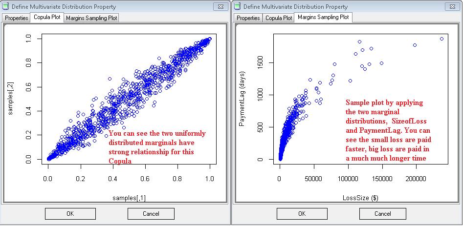
73 The word copula derives from the Latin noun for a "link" or "tie" that connects two different things. In statistics, a copula is a multivariate probability distribution for which the marginal probability distribution of each variable is uniform. Copulas are used to describe the dependence between random variables Consider a random vector. Suppose its margins are continuous, i.e. the marginal CDFs are continuous functions. By applying the probability integral transform to each component, the random vector has uniformly distributed marginals. The copula of : is defined as the joint cumulative distribution function of Let us use an example to see how Copula is implemented in ReservePrism. Under the Severity section from Type, you can set the Size of Loss and Payment Lag correlation, which could mean you usually pay out large loss in longer settlement time. Let us define a strong normal Copula with correlation matrix as: 72

74 73

75 Distribution Fitting Tools Distribution Fitting Tool This tool has common distribution fitting user interface to load and fit any data to Homogenous, Heterogeneous, or Mixture distributions. As usual, data should be prepared in CSV file, and date format should go with international date format such as You can drag top columns and drop them to the bottom for observations. The second tab will show the observation empirical graphs. You fit the data on third tab. Copula Fitting Tool Besides Copula fitting on Size of Loss and Payment Lag from real claim data, this Copula Fitting Tool provides a convenient way to test any sets of correlated data. Step 1, load data in CSV format. The file should contain columns of correlated data. In our example, we have 2 columns of data (from 2 correlated lognormal distributions) 74

76 Step 2: Pick a Copula family, Marginal Distribution Families, and then click Fit Step 3: The fitted Copula parameters and plots will be filled on screen. 75

77 76

78 Mixture Distribution Fit ReservePrism uses the Expectations-Maximization (EM) algorithm to maximize the likelihood function of the mixture distribution. You pick the distribution family, ReservePrism depicts you with the best fit, and provides random sample from the model as well. Convenient Stochastic Utilities PLEASE NOTE THAT NEITHER BOOTSTRAPPING NOR LDF CURVE FITTING METHOD IS PROMOTED BY RESERVEPRISM FRAMEWORK. We provided these traditional simulation tools since we already developed the core R library within the system. 2-Stage Bootstrapping Prepare your Paid Loss Triangle in CSV (comma separated text) file format, and make sure to remove the possible comma separator for dollar amount. Load the Paid Loss triangle to Bootstrap utility. 77

79 All the intermedia steps, like Fitted Incremental, ChiSqr, and Residual, etc, are shown instantly. Then simply select what you prefer for output and click Run. You can copy and paste the percentile result or you can also export the result to CVS file. 78

80 LDF Curve Fitting Prepare your Paid Loss Triangle in CSV (comma separated text) file format, and make sure to remove the possible comma separator for dollar amount. Then load the Paid Loss triangle to LDF Curve Fitting utility. 79

81 Select growth function and click FitCurve button. The result table below compares the (Fitted) Ultimate Loss and Reserves from the Fitted All Year Weighted LDF factors (based upon your selected growth function) and the results from the normal Paid Loss analysis. 80