THE FEDERAL DEMOCRATIC REPUBLIC OF ETHIOPIA CENTRAL STATISTICAL AGENCY HOUSEHOLD CONSUMPTION AND EXPENDITURE (HCE) SURVEY 2010/11 ANALYTICAL REPORT

Transcription

1 THE FEDERAL DEMOCRATIC REPUBLIC OF ETHIOPIA CENTRAL STATISTICAL AGENCY HOUSEHOLD CONSUMPTION AND EXPENDITURE (HCE) SURVEY 2010/11 ANALYTICAL REPORT October 2012 Addis Ababa 563 STATISTICAL BULLETIN 563

2 LIST OF TABLES II LIST OF FIGURES III EXECUTIVE SUMMARY 1 1. INTRODUCTION AND OVERVIEW 3 CONCEPTS AND DEFINITIONS 6 AREA OF RESIDENCE 6 HOUSEHOLD CHARACTERISTICS 7 EMPLOYMENT AND ENTERPRISE 8 HOUSEHOLD EXPENDITURE 8 CALORIC ANALYSIS SURVEY DESIGN COVERAGE SAMPLING FRAME SAMPLE DESIGN & SELECTION DATA COLLECTION & PROCESSING DATA COLLECTION FIELD SUPERVISION DATA PROCESSING DATA ENTRY AND CODING DATA VALIDATION AND CLEANING MAJOR FINDINGS AND ANALYSIS SOCIO-ECONOMIC INDICATORS POPULATION HOUSEHOLD SIZE AND COMPOSITION HOUSEHOLD HEAD INCOME CONTRIBUTING MEMBERS LITERACY AND EDUCATION ECONOMIC ACTIVITIES EXPENDITURE EXPENDITURE PER CAPITA EXPENDITURE BY ITEM CATEGORY SUPPLEMENTARY EXPENDITURE ANALYSIS SOURCES OF EXPENDITURE CALORIC CONSUMPTION CONCLUSIONS REFERENCES ANNEXES 77 ANNEX I: DISTRIBUTION OF SAMPLING UNITS 79 ANNEX II: EQUIVALENCE SCALES FOR CALORIE ANALYSIS 85 ANNEX III: SPATIAL PRICE INDEX 87 ANNEX IV: PROBIT REGRESSION RESULTS 89 ANNEX V: 2010/11 HCE QUESTIONNAIRE 91

3 List of Tables Table 1: Household Expenditure Quintiles (Country Level) 9 Table 2: Data Categories and Related Reference Periods 16 Table 3: Distribution of Regional Populations by National Household Expenditure Quintile 21 Table 4: Regional Population Distribution - by Sex and Residence 22 Table 5a: Percentage Distribution of Population by Household Size (% of Individuals) 25 Table 5b:Distribution of Population Disaggregated by Expenditure per Capita Quintiles (%) 25 Table 6: Household Size and Age Decomposition by Region 26 Table 7: Distribution of Population by Age and Quintile (%) 28 Table 8: Proportion of Female Headed Households by Quintile (% of Households) 30 Table 9: Population by Sex (% of population that is female) 31 Table 10: Income Contributing Household Members 32 Table 11: Age Decomposition, Country Level 34 Table 12: Literacy Rates by Quintile and Sex 35 Table 13: Population (aged 13 and above) that have completed Advanced Primary School 36 Table 14: Household Head Education 37 Table 15: Household Head Employment Status (%) by Quintile 40 Table 16: Distribution of Employment Status by Region 42 Table 17: Head of Household Industry (%) 43 Table 18: Primary Industries 44 Table 19: Occupation of Active Household Heads 45 Table 20: Type of Unemployment by Expenditure Quintile 46 Table 21: Expenditure Per Capita by National Household Expenditure Quintiles 48 Table 22: Expenditure per capita by Expenditure per Capita Quintiles 48 Table 23: Expenditure per Capita - Alternative Measurements 50 Table 24: Expenditure per Capita Over Time 52 Table 25: Distribution of Expenditure by Region 53 Table 26: Expenditure Per capita by Major Item Group 54 Table 27: Regional Expenditure by Major Item Group 55 Table 28: Expenditure per Capita for Selected Items 57 Table 29: Expenditure Allocation by Expenditure per Capita Quintiles 60 Table 30: Budget Allocation by Sex of Household Head 61 Table 31: Household Expenditure by Highest Head Education 62 Table 32: Distribution of Household Expenditure by Source (%) Country Level 65 Table 33: Distribution of Household Expenditure by Source (%) - Regional Level 67 Table 34: Expenditure Sources by Type and Sex of Household Head 68 Table 35: Daily Calorie Intake per Adult Equivalent by Food Group and Place of Residence 70 Table 36: Daily Gross Calorie Intake per Adult Equivalent by Food Group and Quintile 71 Table 37: Regional Daily per Capita Calorie Intake Across Time 72

4 List of Figures Figure 1: Population by Household Expenditure Quintile 22 Figure 2: Trends in Dependency Ratios 29 Figure 3: Proportion of Female Headed Households 30 Figure 4: Income Contributing Household Members 33 Figure 5: Literacy Rates 34 Figure 6: Literacy by Region 36 Figure 7: Grade 6 Completion 38 Figure 8: Expenditure Allocation (Meat & Rent) 58 Figure 9: 2010/11 Expenditure Allocation (Alcohol, Tobacco, and Chat) 59 Figure 10: Daily Gross Calories by Food Group 71 Figure 11: Daily Gross Calories per Capita 73

5 Executive Summary The Household Consumption and Expenditure (HCE) survey is administered by the Central Statistical Agency every five years, most recently in 2010/11. This report intends to provide a general understanding and analysis of the levels and distributions of major indicators as well as a look into the trends across previous periods. A similar analytical report was completed in 2007 for the 2004/5 HICE survey (Central Statistical Agency, 2007). The current study uses this 2004/5 analysis as a baseline for change as it also includes data from the previous two HICES (1995/6 and 1999/0). A further statistical report will be separately released by the Central Statistical Agency. Using the expenditure data from the 2010/11 HCE survey, a variety of indicators are measured. These are generally disaggregated into socio-economic indicators, expenditure levels and sources, and caloric consumption. While the majority of trends, distributions and levels remain similar to those seen in previous years, there have been clear improvements in areas such as literacy, education, and calorie consumption. The national population has grown to an estimated 76.1 million, an increase of 17.5% since 2004/5. The national average household size has remained almost constant at 4.8 since 2004/5 but the average rural household size has increased slightly to 5.1 from 4.9 persons while the average urban household size has fallen to 3.7 (a decrease of 14% since 2004/5). The nationwide dependency ratio is decreasing, implying that a greater percentage of the population is of working age. Literacy and education levels are on the rise, with 48.3% of the total population age 10 and above able to read and write (compared to 37.6% in 2004/5). Much of this growth was enjoyed by females, especially those in the upper expenditure quintiles. Although there is still a gap in the education and literacy of males and females and between urban and rural populations, the 2010/11 HCE data shows improvements for all groups. The education of both males and females has increased. Grade 6 completion rates for household heads, for example, increased from 7.1% to 10.2% for females and from 11.3% to 15.6% for males from 2004/5 to 2010/11.

6 Expenditure values have increased significantly, although this is very strongly related to the high levels of inflation experienced in Ethiopia over recent years. Expenditure patterns are very similar to those observed in previous years, with households in the lower expenditure quintiles allocating a greater share to food and other basic goods while those in the higher quintiles devote a greater share to relatively more expensive items such as meats, alcohol and clothing. Calorie consumption has clearly improved as the average daily per capita gross calorie consumption is up to 2,455 from the 2004/5 average of 2,353 (and only 2,211 in 1999/0). As in previous years, caloric intake is greater for rural populations, likely due to their ability to consume their own agricultural produce. The following report looks at each of these indicators, in addition to others, in greater depth and attempts to explain the relationship of each with relative household expenditure levels.

7 1. Introduction and Overview Although poverty has continued to be at the forefront of Ethiopian concerns, recent history shows great improvements. The incidence of poverty has declined from 45.5% in 1995/6 to 38.7% in 2004/5 and finally to 29.6% in 2010/11 (Ministry of Finance and Economic Development, 2012). Signs of this reduction in poverty as measured by the Ministry of Finance and Economic Development (MoFED) is evident in this analytical report of the 2010/11 HCE survey data through improvements in literacy, education, and per capita expenditures among others. The government of Ethiopia, together with development partners, has implemented various poverty reduction strategies to promote economic growth in recent years. The latest sustainable growth strategy, the Growth and Transformation Plan (GTP) covers the period from 2010/ /15. This plan focuses on seven strategic pillars including, but not limited to, sustainable and equitable economic growth, maintaining a focus on agriculture, improving social development and promoting gender and youth empowerment. The GTP was preceded by the Plan for Accelerated and Sustainable Development to End Poverty (PASDEP, 2005/6-2009/10) and the Sustainable Development and Poverty Reduction Program (2002/3 2004/5). The GTP aims to extend the functions of the PASDEP and achieve the Millennium Development Goals by 2015 as well as realize middle-income country status by (Ministry of Finance and Economic Development, 2010). The HCE survey plays an integral role in achieving the aims of the GTP and the MDGs by enabling thorough monitoring and evaluation of key indicators. Monitoring and evaluation is critical to the success of poverty-reduction and welfare enhancing programs. Without a sound system in place, the impact of such programs cannot be observed and resources may be incorrectly allocated across programs or populations. To this end, the Welfare Monitoring System (WMS) was established in 1996 to ensure changes in poverty indicators are consistently known and evaluated and the impact of ongoing reform programs are measured (Ministry of Finance and Economic Development, 2012). In order to attain the aforementioned goals, data must be collected periodically. The Central Statistical Agency (CSA) is responsible for the two primary data collection efforts: the Household, Income, Consumption

8 and Expenditure (HICE) and Welfare Monitoring (WM) surveys. Both nationally representative surveys have been conducted together at four or five year intervals since 1995/6, the onset of the Welfare Monitoring System. The HICE survey focuses on the income dimension of poverty through measurement of consumption, expenditure and income, while the WM survey specializes in the non-income aspects of poverty such as health, education, and access to services. Together, the two surveys paint a complete picture of the poverty and welfare environment of Ethiopia. The primary objectives of the HICE survey, the focus of this report, revolve around knowledge building, monitoring current levels and trends in income poverty, and evaluating the impacts of poverty-reducing strategies. To identify further, the objectives include: Assessing the level, extent and distribution of the income and expenditure dimensions of poverty; Providing data on household expenditure patterns, values and distributions at nation and regional levels in order to observe trends in living standards and welfare; Providing data for use in the design, monitoring and evaluation of strategic programs and reforms; Providing estimates of household consumption expenditure for the compilation of national accounts; and Obtaining weights and other necessary information for the construction of consumer price indices at various geographic levels. Periodic collection of HICE and WM survey data allows for analysis in welfare trends over time. The CSA has collected and published reports on the 1995/6, 1999/2000, and 2004/5 HICE and WM surveys. 1 In addition to the analytical and statistical reports produced by the CSA, the Ministry of Finance and Economic Development (MoFED) has produced a number of in depth poverty analyses using the same data. MoFED has also recently released interim poverty analysis using the latest 2010/11 data (Ministry of Finance and Economic Development, 2012). 1 Available on the CSA website.

9 The focus of this analytical report is the latest 2010/2011 HCE survey. In contrast to previous years the income component was not captured, making the 2010/2011 an HCE survey rather than an HICE survey. The value of income data, particularly in developing economies, is typically very low and thus little was lost by the exclusion of this survey section. Income data can be quite difficult to collect, especially when a large portion of the population is engaged in subsistence agriculture. Furthermore, expenditure and consumption values are widely preferred to income estimates for the sake of welfare analysis (see, for example Deaton & Zaidi, 2002). Using consumption data can fill the gaps of subsistence farming, in-kind transactions, and other components that income tends to significantly exclude in developing economies. Thus, in this analysis (as in previous HICE analysis) we focus on consumption and expenditure, used interchangeably, to assess the state of the Ethiopian population. This report is intended as a broad-based analysis. A detailed statistical report of the 2010/11 HCE data is also to be produced by the CSA and made available online. This report is broken down into four primary sections: Survey Methodology and Data, Socio-Economic Indicators, Expenditure Levels and Sources, and Caloric Consumption.

10 Concepts and Definitions This section serves as a glossary for the following sections, defining terms and clarifying aggregated figures. The terms are grouped by the following categories: area of residence, household characteristics, employment and enterprise, household expenditure, and caloric analysis. Area of Residence Urban Center: An urban center is often defined as a locality with 2000 or more inhabitants. For practical purposes, this survey defines an urban center to include the following (regardless of the population): a. All administrative capitals (region, zone and wereda capitals), b. Localities with Urban Dweller s Areas (UDAs) not included in (a), c. All localities that are not included in (a) or (b) and which have a population of 1000 or more persons and whose inhabitants are primarily engaged in nonagricultural activities. Urban Kebele (UK): The smallest administrative unit in an urban center with its own jurisdiction. It is a locality formed by the inhabitants and usually constitutes a part of the urban center. Rural Kebele (RK): The smallest administrative unit in a settled rural area with its own jurisdiction. It is an association of rural dwellers formed by the inhabitants of an area in which members may or may not be engaged in agricultural activities. Enumeration Area (EA): An area delineated for the purpose if enumerating housing units and population without omission or duplication. An EA generally consists of households in rural areas and housing units in urban areas. An EA is related to an urban or rural kebele in one of the following ways: a. An EA may be equal to a rural kebele if the number of households in the kebele is less than or equal to An EA may be equal to an urban kebele if the number of housing units is less than or equal to

11 b. An EA may be a part of an RK or UK but its delineation cannot extend outside the border of the kebele. Collective Quarter: A premise (a housing unit, building, or compound) in which a number of unrelated persons reside and share common facilities. Examples of collective quarters are monasteries, prisons, boarding schools, military barracks, etc. It is important to note that there may be private households on the premises of some collective quarters. Household Characteristics Household: A person or group of person, whether or not they are related, who normally live together in the same housing unit or group of housing units and who have common cooking arrangements. Head of Household: The person who economically supports or manages the household or, for reasons of age or respect, is considered as the head of the members of the household or otherwise declares him or herself as the head of a household. There may only be one head of household and this person may be male or female. Member of Household: A member of a household may be any of the following: a. All persons who lived and ate with the household for at least six months (including those who were not present at the time of the survey but were expected to be absent from the household for less than six months). b. All guests and visitors who ate and stayed with the household for six months or more. c. Housemaids, guards, babysitters, etc. who lived and ate with the household, even for less than six months. Household size: The total number of members of a household.

12 Employment and Enterprise Unincorporated Household Enterprise: An economic enterprise where goods and services are produced for sale. This also includes those engaged in strictly buying and selling activities. Generally the type of enterprise considered as an unincorporated household enterprise is an enterprise run by the household or a household member in which the primary aim of the enterprise is to manage the livelihood of the household. In such enterprises, there is no distinct difference between the enterprise s income/expenditure and the household s income/expenditure. Productive Activity: An act of selling the output of an activity in kind or in cash. This includes, but is not limited to, working at an enterprise for wages/salary and working on rural agricultural activity (even if for own private consumption). Employer: A person who hires at least one employee for his/her enterprise or activity. A person who uses hired labor and takes part in the productive activity is considered an employer. Self-Employed: An individual who works in his own enterprise including agriculture (without hiring any labor). For the purposes of this survey, those who use only family labor without payment are considered self-employed. Unpaid Family Worker: A member of a household who is working for the enterprise or activity of the household without payment. Household Expenditure Consumer Goods and Services: Goods and services used by a household to directly satisfy the personal needs and wants of its members. Household Consumption Expenditure: Value of consumer goods and services acquired, used or paid for by a household through direct monetary purchases, own account production, barter, or as income in kind.

13 Actual Final Consumption: The sum of a household s consumption expenditure plus the value of goods and services acquired or used through transfers from government, non-profit institutions, other households, etc. Some transfers, such as free education, are extremely difficult to value and have therefore been excluded from all HICE data. Household Expenditure: The sum of household consumption and non-consumption expenditures. Non-consumption expenditures are those that are incurred by a household without receiving any goods or services in return (ignoring any potential goodwill). Examples of such transfers may be gifts, donations, compulsory fees or fines and taxes (if no services are received in return). Household expenditure represents the total outlay made by a household in a given period (in this case, one year). Household Expenditure Quintiles: The household expenditure quintiles are used to disaggregate households by total household expenditure levels. The quintiles are calculated by first ordering all households in ascending order by value of household expenditure and then dividing them into five equal parts such that the first group includes the 20% of households with the lowest annual expenditure and the last group includes the 20% of households with the highest annual household expenditure. The values of each national household expenditure quintile are reported in Table 1.

14 Expenditure per Capita Quintiles: While the majority of analysis uses the above Household Expenditure Quintiles, some sections include the use of expenditure per capita quintiles. These quintiles are constructed by first calculating the annual value of expenditure per capita (total household expenditure divided by the number of people in the household). Households are then ranked in order from lowest per capita expenditure to highest and then grouped such that the 1 st expenditure per capita quintile includes the 20% of households with the lowest expenditure per capita. Per Capita: Per capita is simply per person, counting all adults and children the same. Per Adult: In the expenditure section, adult equivalents are sometimes used to account for the difference between the cost of children and adults as well as consider any economies of scale gained from household public goods. The formula used to calculate the number of adult equivalents per household comes from the often-cited Angus Deaton and Salman Zaidi and is footnoted in section (Deaton & Zaidi, 2002). Expenditure is divided by the number of adult equivalents to arrive at the expenditure per adult. In the calorie analysis, adult equivalent has a different meaning. In this sense, the adult equivalent calculation is used to consider the difference in caloric needs from different people. The adult equivalence scale for use in calorie analysis has specific values for people of varying ages and sexes. The scale used here was adopted from the Ministry of Finance and Economic Development (who calculated this from Dercon & Krishnan, 1985) (Ministry of Finance and Economic Development, 2008). The scale is attached in Annex II. N/A: Not Applicable or Not Available. Caloric Analysis Adult Equivalent: see above. Gross Calorie: The total number of kilocalories in a given weight of food product, prior to discarding any inedible materials. These are determined based on the food composition tables

15 calculated by the Ethiopian Health and Nutrition Research Institute (ENHRI) and the Food and Agriculture Organization of the United Nations, Net Calorie: The total number of kilocalories in a given weight of food after removing the inedible portions. It is the gross calorie deflated by (or minus) the proportion of the inedible material, termed as refuse. Also derived from the food composition tables calculated by ENHRI (Ethiopian Health and Nutrition Research Institute and the Food and Agriculture Organization of the United Nations, 1998). Refuse: Refuse refers to the percentage of the total purchased/produced weight that is discarded while preparing food. Refuse includes bones, pits, shells, and other inedible portions that could be eaten but as a rule are discarded (potato parings and tough outer leaves of vegetables, for example).

16 2. Survey Design 2.1 Coverage The 2010/11 HCE survey covered all rural and urban areas of the country except the nonsedentary populations in Afar (three zones) and Somali (six zones). Initial sample selection included 864 rural EAs and 1,104 urban EAs, with 10,368 and 17,664 households respectively. For various reasons, 2 rural EAs and 48 rural households were not surveyed, resulting in a rural household response rate of 99.5%. All selected urban EAs were successfully covered with an urban household response rate of 99.2%. 2.2 Sampling Frame The 2007 Population and Housing Census served as the sampling frame from which the rural and urban EAs were selected. A fresh list of households for each selected EA was collected at the beginning of the survey period. Households were then selected for inclusion in the survey by choosing a random number as the starting point in the list and selecting every nth household (n being the necessary number to achieve the desired number of households in each EA). 2.3 Sample Design & Selection In order to produce a representative sample, the country was stratified into the following four categories: rural, major urban centers, medium towns, and small towns. a. Category I Rural This category consists of the rural areas of 68 zones and special weredas, which are considered zones, in 9 regions of the country. This category also includes the rural areas of the Dire Dawa City Administration. A stratified two-stage cluster sample design was used, with the primary sampling unit being the EAs. Sample EAs were selected using Probability Proportional to Size, with size being the number of households identified in the 2007 Population and Housing Census. Twelve households were randomly selected from each sample rural EA for survey

17 administration. The total sample for this category is 864 EAs and 10,368 households. b. Category II Major Urban Centers This category includes all regional capitals as well as five additional major urban centers with large populations, for a total of 15 major urban centers. These 15 urban centers were broken down into the 14 regional capitals and the 10 sub-cities of Addis Ababa City Administration resulting in a total of 24 represented urban domains. A stratified two-stage sample design was also used for this category as in the rural sample with EAs as the primary sampling unit. For this category, however, 16 households were randomly selected in each EA. In total, 576 EAs and 9,216 households were selected for this category. c. Categories III & IV Other Urban Centers These two categories capture other urban areas not included in Category II. A domain of other urban centers was formed from 8 regions (all except Harari, Addis Ababa, and Dire Dawa where all urban centers are included in Category II). Unlike the other categories, a three-stage sample design was used. However, sampling was still conducted using probability proportionate to size. The urban centers were the primary sampling units and the EAs were secondary sampling units. Sixteen households were randomly selected from each of the selected EAs. A total sample of 112 urban centers, 528 EAs, and 8,448 households were selected for these two categories. In total, 66 reporting levels were created under this sampling design. The distribution of samples by region is detailed in Annex I. A copy of the questionnaire is found in Annex V.

18 3. Data Collection & Processing The Branch Offices Desk at the head office led CSA branch offices in the organization of fieldwork. All 25 branch offices of the CSA fully participated in the survey activities, from recruitment of field staff to field supervision to providing completed questionnaires to the head office. Each branch office was responsible for financial and logistical arrangements as well. Local government offices, especially at the Kebele level, played a vital role in facilitating fieldwork through familiarizing selected households with the survey and enumerators. 3.1 Data Collection Data was collected over the course of one year, from 8 July 2010 to 7 July The CSA branch offices organized a total of 82 data collection teams, which consisted of 2 enumerators and 1 supervisor/field editor. Each of these teams was responsible for administering the HCE survey in at most 24 EAs, with each EA taking roughly 15 days per team. In each rural EA, 12 households were selected, and in each urban EA, 16 households were selected. Two enumerators (one team) were assigned to each EA such that the enumerators each collected data from 6 rural households or 8 urban households per EA. Data was collected in such a way that each household was visited by the same enumerator twice within one week. Enumerators were able to visit 2 households per day in rural areas and 2-3 households per day in urban areas. Including multiple visits to each household was essential to minimizing the effects of recall error. To further check the robustness of the data, a variety of recall periods were used for some variables. For example, each household was asked to estimate their total rent expenditure in the last 3 months as well as the last 12 months. Table 2 summarizes the data categories and respective recall periods. In addition to the HCE, a market price survey was administered simultaneously in markets in or nearest each sample EA. This price data served as a comparison for household-reported values

19 as well as a potential source to complete values when households could not report it themselves (for example, in self-production). 3.2 Field Supervision Regular and thorough supervision is crucial to ensure the integrity and quality of the data. Each field team included one supervisor who was responsible for supervision, field editing, and coordination of activities. Additionally, a statistician was assigned by each CSA branch office to oversee HCE data collection activities. Branch office heads and professionals from the head office were involved in field supervision as well. A team of CSA top management, CSA experts and experts from Finland Statistics observed fieldwork on two occasions during the survey period.

20

21 3.3 Data Processing All data processing was undertaken at the head office. Completed questionnaires were returned to the CSA data processing department from the field periodically. Data processing activities included cleaning, coding, and verifying data as well as checking for consistency. These activities were carried out on a quarterly basis after entering three months of data. Further processing, including the estimation of sampling weights, was carried out at the close of data entry. 3.4 Data Entry and Coding Manual editing and coding of data began as early as August 2010, when the first round of completed questionnaires was received at the head office. A team of 21 editors, 5 verifiers, and 4 supervisors carried out these activities. Subject matter experts provided a 5-day intensive training for this team to equip them with the necessary skills. Additionally, a team of 12 encoders was trained to enter the data. A double-entry system was used, wherein two separate encoders manually entered each survey. Any discrepancies between the two entries were flagged automatically and the physical survey was reviewed to correct the errors. Data entry was completed in October Data Validation and Cleaning Data validation and cleaning was carried out by subject matter experts and data programmers. Systematic validity checks were completed at the commodity, household and visit levels. Activities related to consistency, validity, and completeness included the following: a. Imputation of missing observations on consumption goods (in quantity or value) using the market price survey that was collected at the time of the HCE. b. Validity and consistency of quantity and value of consumption items was checked by comparing the figures across both household visits (using the household provided prices and/or the market price survey).

22 c. Estimation of the value of consumption of own production using the householdprovided quantities and market survey prices. d. Comparison of household expenditure on durable goods using different recall periods (i.e., 3 and 12 months). After analyzing the annualized values using each reference period, it was decided to use whichever period resulted in the largest expenditure, which was often the shorter recall period. The logic behind doing so is that households are more likely to forget to include items the more time has elapsed since the consumption. All phases of data processing were completed in February 2012.

23 4. Major Findings and Analysis The major findings of the 2010/11 HCE survey are broken down into three larger categories, namely socio-economic indicators, expenditure levels and sources, and caloric consumption. As the focus of the HCE survey is on expenditure and the income dimensions of poverty, the analysis attempts to describe the relationship of each indicator with relative household expenditure levels. Many of the tables found in the following sections are disaggregated by total household expenditure quintile. Such disaggregation allows for comparison of households relative to the total population of households. When examining trends over time with quintile groups, it is important to note that the expenditure range associated with each quintile in different years is not the same. Rather, we are comparing the poorest 20% of households in 2004, for example, to the poorest 20% of households in It is also crucial to recognize that the quintiles are constructed based on total household expenditure, not expenditure per capita. As will be discussed in the text below, this can cause smaller households to be pushed into the lower quintiles. For the sake of comparability with the 2004/5 analytical report, this report will also focus on household expenditure quintiles but in certain sections, additional analysis is executed using quintiles of expenditure per capita in order to clarify the conclusions being made (the tables will be labeled accordingly). For clarification, quintile 1 encompasses the 20% of households with the lowest annual expenditure and quintile 5 the 20% of households with the highest. By using sample weights and accounting for design effects, it is possible to extrapolate the survey data to the national population (less the non-sedentary populations that were excluded from the survey for practical reasons). All of the tables and figures in this analysis have been weighted so they reflect the entire population, not only those that were surveyed.

24 4.1. Socio-Economic Indicators Population The first step in assessing changes within a population is looking at the size of the population itself. Using the 2010/11 HCE data, the population is estimated to be 76.1 million people 2. The results of the 2004/5 HICE survey concluded that the national population was 64.5 million people, although this excluded the Gambella region in addition to the aforementioned nonsedentary areas. After accounting for the exclusion of Gambella, this shows a 17.5% increase in the population over the last five to six years, and a roughly 35.3% increase since the 1999/0 HICE. It is evident that population growth has increased, as the five to six year increase from 1999/0 to 2004/5 was only about 15.2% (Central Statistical Agency, 2007). The proportion of males and females has remained constant and evenly distributed, with 49.4% male and 50.6% female. There has been a slight shift in the proportion of urban and rural persons, however. In 2010/11, the data shows that 83.4% of people resided in rural areas and 16.6% in urban areas. In 2004/5, a larger percentage of people were rural dwellers (85.7%). Because the majority of the following analysis uses the national household expenditure quintiles, Table 3 is included to provide context. This table supplies the proportion of individuals in each region by national quintile. These quintiles are not constructed on a regional basis so there are not even distributions across quintiles at the regional level. For example, in Tigray only 11.3% of individuals within that region are in households of the 1 st quintile. In Addis Ababa, there is a very large concentration of the population in the 5 th quintile (64.3%) and only a very small proportion in the 1 st (2.6%). The regions that make up the majority of the population have distributions most similar to the 20% allocation in each quintile. These regional distributions will serve as useful reference points in the following analysis. 2 Population in this report refers to the nation population less the non-sedentary regions identified in section 2.1.

25 Also relevant is the distribution of rural and urban populations across these national household expenditure quintiles. Figure 1 provides a distribution of the population in total as well as by rural and urban populations across quintiles. Because these groups are constructed by household rather than by individual, there is not an even 20% of the population in each. There are slightly fewer individuals in the lower quintiles because, as discussed below, the average household size tends to be smaller. Nonetheless, there is a fairly even division on the whole. The urban population, however, is much more concentrated in the upper quintiles. The rural population is very close to evenly distributed because they make up over 83% of the national population. As an additional reference, Table 4 provides the regional distribution of urban/rural and male/female populations.

26

27 4.1.2 Household Size and Composition In line with previous analyses, rural households are larger than urban households on average. In 2010/11, rural households had on average 5.1 people while urban households had only 3.7 people. In 2004/5, these numbers were 4.9 and 4.3, respectively. On a national level, the average number of people in a household in 2010/11 was 4.8, the same as the 2004/5 average. Although the national average size remained constant, the average rural household size increased by 4% while the average urban household size decreased by 14%. Table 5a looks at the distribution of household size by place of residence and annual household expenditure quintile. The table identifies the percentage of the population in each group. For example, 22.3% of all urban dwellers in the first household expenditure quintile live in singleperson households while only 8.2% of the same group lives in households of 5 people. Looking at this table alone, we could conclude that poorer households, those in the lower quintiles, more often have small household sizes compared to those in the higher quintiles. At the national level, in the first quintile, only 1% of people live in households of 10 or more people. In the fifth quintile, however, 14% of people live in households of 10 or more. There appears to be a gradual shift towards higher household size with increasing quintiles. In comparison to the analytical report of 2004/5, the trends are similar but there is a clear shift in the urban population. Fewer urban dwellers fall in the right extreme, with only 4.3% of the urban population living in households of 10 or more, compared to 7.8% in 2004/5. At the same time, the proportion of urban people in the low-medium sized households has increased. In 2004/5 the percentage of urban dwellers was 15.3% in households of 4 and 16.6% in households of 5. In 2010/11, these figures are 17.2% and 17.4% respectively. The most obvious of the changes to the urban distribution is the dramatic increase in the percentage of single-person households, particularly in the 1 st and 2 nd quintiles. In 2004/5, the percentage of urban dwellers in the first quintile in single-person households was only 9.2% compared to the 22.3% seen in 2010/11. In terms of the rural population, the distribution of individuals is largely the same as found in 2004/5 but with a slightly more even distribution across household sizes. For example, in 2004/5, 21.6% of rural individuals in the first quintile lived in households of 4 people (the category with the highest concentration of individuals). In 2010/11, this figure is only 17.5%

28 and this is the highest concentration (that is, no other household size includes more than 17.5% of the rural, first quintile population). Analyzing household size by annual household expenditure quintile can be misleading on its own. Because these are constructed based on the total household value rather than a per capita value, smaller households may be artificially pushed into the lower quintiles. Smaller households have fewer people to feed (therefore, fewer expenditure needs) and fewer potential income earners (therefore, fewer means to meet those needs), thus their annual expenditure may be naturally lower. Simply because their expenditure is less, however, does not necessarily make them worse off. For example, a single person household has one earner and one mouth to feed. If this person earns Birr 1000 per year they are quite possibly better off than a two-person household that earns Birr 1500 per year. To complete the analysis of household size with respect to expenditure, we also examine the size in relation to expenditure per capita quintiles. These quintiles, in contrast to the annual household expenditure quintiles, are constructed by first dividing the annual household expenditure by the number of people in the household (achieving the expenditure per capita) and then creating 5 groups of households by their expenditure per capita. This is still not a perfect measure as there are things like household public goods and economies of scale that are not reflected here but it is an improvement nonetheless. In the expenditure section, we attempt to account for these economies of scale and other factors. Table 5b duplicates 5a but disaggregating by expenditure per capita quintiles. Table 5b paints a very different picture. When using expenditure per capita, the relationship is clear that individuals with lower per capita expenditures come from larger households. The opposite is also true; individuals with the highest expenditure per capita often reside in smaller households. This trend holds true for both urban and rural populations, with rural populations generally shifted towards the right with higher households sizes. The differences in Table 5a and 5b illustrate the need to fully recognize the context and dimensions of the analysis, as the conclusions may be vastly different. Here, we can conclude that on a strictly household expenditure basis, the households with the lowest total expenditure tend to be smaller while on a per capita basis larger households often encompass the individuals with the lowest per capita expenditure.

29

30 Table 6 provides the average household size by region. It is not surprising that the regions and city administrations with primarily urban populations have the smallest household sizes. Addis Ababa, for example, which is considered 100% urban in this survey, has the smallest household size at 3.93 people. This has actually decreased by 19.8% from 4.9 people in 2004/5. Somali region, which is 81% rural, has the largest average household size at 5.33, up from 4.8 people in 2004/5. Of greater interest in Table 6 is the dependency ratio and decomposition of age groups. The dependency ratio is calculated at the aggregate level in each region as well as for all urban and rural areas. By dividing the number of non-working aged persons (younger than 15 and older than 64) by the total number of working aged persons (ages 15 to 64) we arrive at the dependency ratio. This figure gives an approximation of the ratio of income earners to those non-earners who rely on others to fulfill their needs. A dependency ratio greater than 100 implies that there are more dependent people (younger than 15 and older than 64) than there are working-aged people.

31 In all regions but Afar and Gambella, rural dependency ratios exceed 100. This is to be expected, as the rural areas are where larger household sizes are seen. Urban dependency ratios are less than 100 in all regions except for Somali, the region that has the largest average household size. Addis Ababa has the lowest overall dependency ratio at 41.16, meaning that every 100 people of working age have dependents. Again, this is what we would expect given that Addis Ababa is considered 100% urban in this survey and has the smallest average household size. By breaking down the population into age groups, it is evident that the higher dependency ratios are driven by a high percentage of younger people, rather than those over 64. In the primarily rural regions, such as Oromiya and SNNP, the percent of the population below age 15 is nearly 50%. In Somali, where we see the highest dependency ratio, over half of the population is younger than 15. In all regions except Addis Ababa at least 16% of the population is younger than 6 years of age. The distribution of individuals across age groups has remained fairly consistent since Of note is the increase in the Somali proportion of persons below age 10. In 2004/5 this was 33.8% and has risen to 38% in 2010/11. Dire Dawa has experienced a similar increase, with 24.8% younger than 10 in 2004/5 and 27.6% in 2010/11. Although the overall proportion is relatively small, the percent of the population above age 64 has increased from 2004/5 in most regions. The national level dependency ratio is This reduction from the 2004/5 ratio of 102 is largely attributable to the decreased proportion of young persons (the proportion of elderly has slightly increased). A decrease in the urban dependency ratio from 64.7 in 2004/5 to in 2010/11 coupled with the slight shift in overall population from rural to urban also helps to explain this decrease in the national dependency ratio. In order to examine the relationship between dependency ratios, age distribution and relative expenditure, Table 7 breaks down the national population by household expenditure quintile. In terms of age distribution, there is a slight increase in the proportion of young people with increasing quintiles. The opposite is true with the older population; the lowest quintile has the highest proportion of people over 64 and the percentage decreases with increasing quintiles. This can be partially explained by the high percentage of single person households in the first

32 quintile observed in Table 5a (these single person households are not likely to be made up of children). The relationship between dependency ratio and household expenditure quintile is not entirely obvious. It is apparent that urban ratios are significantly lower than rural ratios at all expenditure levels, with the greatest difference between the two being in the 3 rd and 4 th quintiles. There are no clear trends in the dependency ratios themselves, however. The proportion of the population in working-age range remains fairly consistent in all quintiles (about 63% in urban and 48% in rural areas). The increasing proportion of children that is seen with increasing quintiles is offset by smaller proportions of those above working age. Without much variation in the fraction of household members that are likely to contribute to income across quintiles, the dependency ratios will remain steady.

33 The HICE survey series has allowed for measurement of dependency ratios over time. Figure 2 graphs the trend in national, urban, and rural dependency ratios. Prior to 2004/5, the rural ratio was increasing, which in turn drove up the national average. In 1995/6, the rural ratio was It increased to in 1999/0 and to in 2004/5. Over the ten-year period from 1995/6 to 2004/5, the 6% growth in the dependency ratio was due to the increasing proportion of the population coming from the younger age group (47.5% in 1995/6 and 49% in 2004/5). Since 2004/5, the change in the rural dependency ratio has leveled off, remaining constant at about 110 (the proportion of young people being 48.5% in 2010/11). Urban dependency decreased from 77.3 in 1995/6 to 72.4 in 1999/0 to 64.7 in 2004/5. The percentage change from 1995 to 2004 was 16.3% (negative). The change in the urban ratio from 2004/5 to 2010/11 was 8.6%, a slower decline than the previous five-year period. This decline over time is attributable to the gradually decreasing proportion of young persons in the urban population (40.1% in 1995/6 and 33.8% in 2010/11, the proportion of elderly persons has remained relatively constant) Household Head While the relationship between annual expenditure level and dependency ratio is not distinct, the relationship between the expenditure level and the sex of the household head is quite pronounced. Table 8 illustrates the proportion of households in each quintile that are headed by females. The negative relationship between female-headed households (FHH) and expenditure level is evidenced by the continuous decline in proportion of FHH with increasing quintiles. Nationally, 25% of all households are headed by females. The lowest two quintiles have proportionately more, with 43% of all households in the first quintile being FHH. Only 15% of those in the highest quintile are headed by females. Although the difference here is staggering, it is an

34 improvement over the distribution seen in 2004/5 where 49.5% of first quintile households were headed by females. This negative relationship holds true even when we disaggregate households by urban and rural areas. 37% of all urban households and 22% of all rural households are headed by females. In comparison to 2004/5, there is a slightly greater proportion of female-headed households in the lowest urban quintiles (60.7% in quintile 1 in 2004/5 compared to 64.4% in 2010/11) and a smaller percentage in lower rural quintiles (47.4% in quintile 1 in 2004/5 compared to 41% in 2010/11). The national averages, however, are practically unchanged over the five-year period (38.6% of urban households and 23% in rural households in 2004/5, 25.5% overall).

35 The unequal distribution of female-headed households by expenditure quintiles is seen in varying degrees across regions. Figure 3 is a scatterplot of the proportion of households that are headed by females in each region and by expenditure quintile. The circles represent the lowest quintile and the squares the highest quintile. The gap in the percentages seen between the 1 st and 5 th quintiles was clear from the tables above. However, looking at Figure 3 highlights the dramatic difference observed even between the 1 st and 2 nd quintiles. In all regions but Afar and Gambella, the proportion of FHH in the lowest quintile exceeds that of all other quintiles. Some regions have a tighter distribution than others. In Gambella, for example, the proportion only ranges from 26% to 42% whereas the range in Harari is from 22% to 71%. Although the range in Harari is quite large, it appears there is a gradual change from quintile to quintile as opposed to Tigray or Amhara, for example, where the 1 st quintile is significantly higher than the others, which are clustered more closely. In looking at urban areas compared to rural areas, there is a smoother reduction in the percentage of FHHs by quintile (the gap between the 1 st and 2 nd quintiles is much higher relative to the change between other consecutive quintiles in rural areas). Not only are female-headed households found in higher concentrations at lower quintiles, the proportion of individual females themselves is higher in the lowest quintile. Table 9 sums the female percent of the population by quintile. In 2004/5 the percent of the rural population that was female was 56.7% in the lowest quintile and 52% in the 2 nd quintile, implying the distribution of sex in rural populations has evened out slightly in the lowest quintiles. The national averages and urban distribution are virtually unchanged from 2004/5.

36 4.1.4 Income Contributing Members Analysis of the dependency ratio provides an approximation of the percent of the household that is potentially involved in income-earning activity. The HCE survey allows for estimation of the actual portion of the household that is involved in this type of activity as well as the ages of those people. The questionnaire asks whether each member has contributed to household income (either in cash or in kind) in the 6 months preceding the survey. Coupling that question with the household roster that identifies age, sex, education, etc. of each member provides a rich dataset to analyze the patterns of income-contributing members across quintiles. Table 10 outlines the dynamics of income-contributing members by quintile and place of residence. The percent of members that contribute to household income decreases with increasing annual expenditure quintile. This trend is in line with the average household size by quintile previously discussed. Because households in the lower quintiles are often smaller than those in the top quintiles, it follows that a larger percentage of members would be contributing. In general, the larger the household size, the greater the percentage of children. In a household of 2, for example, at least one person must be a contributing member. In a household of 5, however, you could have 2 contributing members and still have a lower percentage of members contributing. Urban households have a greater percentage of members contributing on average.

37 The percent of contributing members that is male increases with expenditure quintile. In the lowest quintile, 50% of contributing members are male, compared to 62% in the highest quintile. In urban areas, the average percent of male workers is 52% compared to 61% in rural areas. This is could be attributable to the prevalence of female homemaking or child rearing in rural areas. This category of work, although quite necessary and demanding, is not considered to be an income-generating activity in this survey. Figure 4 illustrates the relationship of these figures with household size. It is clear that the percentage of income-contributing members falls as household size increases. There is also a gradual increase in the percentage of contributing members that are male, with larger households having a larger percentage of male contributors. This is in line with the observations made at the quintile level, with higher quintiles having a higher proportion of male contributors. Figure 4 also plots the average age of male and female contributors. For females, the average age in the first quintile and at small household sizes is much higher than that of males (for the 1 st quintile the average age is 39.3 for females and 36.6 for males) and it declines significantly from that point. In the highest quintile, for example, the average female age is only 30.8 and the average

38 male age is The average age of male contributors is fairly stable across household size and quintile. Overall, the average age of male contributors is higher than that of females. This is supported by Table 11, which shows that females begin income-contributing activity earlier than males but they also stop earlier in life. Nationally, 5% of income contributing members are younger than 10, 17% are between 11 and 20, 60% are between the ages of 21 and 51, 12% are between 51 and 65, and 6% are older than Literacy and Education Literacy and education are known to have a strong, positive correlation with welfare. In this section, we examine the apparent relationships between literacy, education and household expenditure quintile. For the purposes of this analysis, literacy is defined as the ability to read and write a short passage in any language. This is measured only for the population aged 10 and above.

39 Literacy rates have seen marked positive changes since 2004/5. Both males and females, urban and rural, have experienced increases in literacy rates. Figure 5 graphs the increases for males and females in both years. Table 12 provides more detailed values. In 2004/5, the national rate was 37.6%. In 2010/11, 48.3% of the population aged 10 and over was literate. Male literacy is higher than female literacy in all quintiles although the gap is narrowing, particularly in the highest quintile. Regional literacy rates are available in Figure 6. The rate varies from 23.3% in Somali to 85.7% in Addis Ababa. Generally, the more urban regions, such as Dire Dawa, Addis Ababa and Harari have greater literacy rates. It is also clear from this chart that rural literacy has made greater strides than urban literacy since the previous HICE survey, but rural areas also have more room for growth. As with literacy, education is positively related to relative household expenditure. Households in the highest expenditure quintile enjoy significantly greater education levels than those in lower quintiles, especially in urban areas. The relationship cannot be deemed causal, as it is likely that education itself increases income (and, therefore, expenditure) and income increases education, particularly for the dependents in the household. That is, if a household has enough income to support its members without children working, those children will be able to attend school instead.

40 In both urban and rural areas, more males are educated than females. Table 13 provides the percent of male and female populations aged 13 years and above that had completed advanced primary school (grade 8 and above) at the time of the survey. Immediately recognizable is the difference between urban and rural education. For rural areas only 4% of people over 12 had completed advanced primary, compared to 39% in urban areas. The difference between males and females is also apparent. In the country as a whole, the rate is 13% for males and 9% for females. In all groups, the rate of education increased with increasing quintiles. The absolute change is less severe in rural areas because the range across all quintiles is quite small (2% in the 1 st quintile to 6% in the 5 th quintile).

41 The education of household heads also exhibits the trend of increasing education with increasing quintile. The difference between the education of male household heads and female household heads within expenditure quintiles is fairly small, with the exception of the 1 st quintile where 8.7% of male heads and 4.2% of female heads have completed grade 6. The grade 6 completion rate for male household heads is higher than that of females in the lowest three quintiles but females have a higher rate than male household heads in the top two quintiles. Table 14 summarizes the education of household heads (as completing grade 6). Although the percent difference between males and females is not glaring, the difference between rural and urban education of household heads is. In urban households, 58.5% of male household heads have completed grade 6 (33.6% of females) and in rural areas only 11.7% of males have completed this level (7% of females). The education of household heads has increased with time. In 2004/5, 10.2% of household heads had completed grade 6 compared to 14.3% in 2010/11. Household heads in the 1 st quintile increased grade 6 completion from 4.9% to 6.8% and those in the 5 th quintile increased from 18.9% to 33.2%. The increase in education is much stronger in the higher quintiles. The disparity between urban and rural education is clear at the regional level as well. Figure 7 displays the regional grade 6 completion rate for the population aged 10 and older.

42 4.1.6 Economic Activities Of the national population 10 years and older, 66.6% are economically active. 3 Their employment status, occupation and industry, however, vary with sex, status in the household and expenditure quintile. The tables below describe the dimensions of employment across these groups. Table 15 disaggregates the employment status of female and male household heads by expenditure quintile. The proportion of household heads, both male and female, that are selfemployed is overwhelming. In every quintile at least 69% of heads declared themselves as selfemployed (the definition of which includes agriculture without hired labor). The concentration of males is greater than females in this category but both are significant. As the expenditure quintile increases, the proportion of self-employed heads decreases slightly (with small increases seen in female heads from the 1 st to 3 rd quintiles), giving way to a greater proportion of 3 Including unpaid family labor. The total estimated population age 10 and above is 51,452,379. Roughly 118,000 were registered without a response in either the economically active or unemployed categories. These people were assumed to not be economically active.

43 employers and those employed in public or private enterprises. The 5 th quintile has a significantly higher concentration of employer and public enterprise/service employees, which may be related to the large concentration of urban households found in this quintile. Also of note is the disparity between the male and female household heads that are not economically active. Overall, 23% of female heads are considered to be in this category. It is important to note that household activities (other than unpaid labor) are not considered an economic activity in this context. This observation is consistent with the trends observed in the income contributing section, where the percent of household contributors that were male increased with quintile. Also in that section we observed that fewer older females are engaged in work than men of the same age. Given that these are household heads, we would expect them to be older and therefore see fewer females engaged in economic activity.

44

45 To assess the breakdown of employment status across regions, we point to Table 16. The employment categories here are the same as in the previous table but these have been reported in more detail. Also note, the percentages given are of all economically active persons age 10 and above, not the entire population of that age. This table also breaks down urban and rural populations at the national level. Looking at this particular disaggregation shows that 94.4% of active rural household heads are self-employed compared to 51% of active urban heads. In addition to self-employment, urban employment is dominated by employment in the public, private and other sectors. Although 13.8% of urban members other than the household head are engaged in unpaid family labor, this number is small in comparison to the 77.1% observed in rural areas. The significant difference between the percentage of household heads and other members engaged in paid activity versus unpaid family labor suggests that the household income is strongly driven by the work of the head, especially so in rural areas. For this reason we will focus primarily on the industry and occupation of the household head in the remainder of the section. The more urban regions, such as Addis Ababa and Harari, have the smallest proportion of household members engaged in unpaid family labor (Harari is 47% urban and Gambella 32%). Dire Dawa has a relatively high proportion of unpaid family labor at 41.9% of active members other than the head given its fairly urban population (68% of households). In comparison to 2004/5, there has been an increase in the proportion of self-employed heads (up to 86.1% from 76% of active heads) and a reduction in the percent that are employers (down to 1.6% from 4.9% of active heads).

46

47 The link between the employment status and industry of household heads fairly clear. Table 17 illustrates the extremely high concentration of household heads in agriculture, which is most likely to be reflective of the large proportion of heads that are self-employed. Those that hire labor as part of their agricultural operation would be considered employers in the table above while those that do not hire labor are considered self-employed. As with self-employment, the proportion of household heads in the agriculture industry is far greater than any other but its dominance is reduced with each quintile, where a smaller portion of heads (both male and female) in the highest quintiles are engaged in agriculture. At the high levels, we see an increase in vehicle services, public administration and defense, and education, likely more urban occupations. When looking at the population as whole (those age 10+ that are economically active) not only household heads, the distribution is relatively unchanged; strong focus on agriculture which declines with quintile and gradual, yet small, increases in vehicle services, education, public administration and defense, as well as hotel and restaurant industries. To take a closer look at the primary industries by region, refer to Table 18. For the purposes of comparison from 2004/5 to 2010/11, the table includes the following consolidated industries: agriculture, hunting and fishing; manufacturing, electric, gas and water; wholesale and maintenance of vehicles; and hotels and restaurants. Other industries that were of significant

48 volume in 2010/11 were defense (1.43% of active people) and personal services (2.97% of active people). Table 18 also includes the male-to-female ratios for the selected industries. Agriculture, the primary industry of the country as a whole is heavily male in all regions but Benshangul, which is nearly even. As a whole, there are 1.35 males in agriculture to every 1 female (this is down from 1.5 males : 1 female in 2004/5). Harari has a particularly high ratio with 5.45 males to every 1 female (this is down from 7.1 in 2004/5). The manufacturing and utility supply industry is predominately female in the country as a whole, but in urban areas where agriculture is less prolific more males are engaged in this industry than females (particularly in Addis Ababa and Dire Dawa). The hotel and restaurant industry as well as the vehicle industry employs more females than males. In the country as a whole, the male-to-female ratios in these industries have remained virtually unchanged, with the exception of a reduction in the urban male to female ratio in agriculture (from 2.2 males: females in 2004/5 to 1.79 in 2010/11) and an increase in the relative number of urban males in the manufacturing and utilities industry (from 0.8 males: females in 2004/5 to 1.03 in 2010/11). In terms of occupation, there are more visible changes over time. Table 19 displays the proportion of economically active household heads by occupation in 2004/5 and 2010/11.

49 In urban areas there was a reduction in the proportion of household heads that were employed as legislators, senior officials and managers. In 2004/5, 8% of active heads were in this category, in 2010/11 only 3%. There was a similar reduction in the craft or trade occupation (from 23% to 14%). The large reductions in these occupations are offset by substantial increases in professional occupations (from 2% in 2004/5 to 7% in 2010/11) and elementary occupations (from 11% to 23%). Additional increases were seen in the percentage of urban household heads employed as services workers or salespersons. In rural areas, the changes were not as large. There was a small shift out of agriculture (from 92% in 2004/5 to 89% in 2010/11) and into elementary occupations. While analyzing the occupations and industries of the economically active population is vital to understanding changes in the Ethiopian environment, it is also worth noting the reasons people are not economically active at all. Table 20 summarizes the reasons or alternative activities that preclude persons aged 10 and above from participating in economic activity. The largest category is education. 53% of people over age 9 that are not economically active have chosen to attend school or training courses. In addition to this 53%, 5.8% noted that they were too young for work. The percent of those that chose education is greater in the higher quintiles while the percentage of those that said they were too young is higher in lower quintiles. The positive progression in education with quintile is in line with the conclusions noted in the education section.

50 The second largest contributor to people not being engaged in economic activity is homemaking. Nationwide, 25.8% of people over age nine that are not economically active consider themselves as homemakers. This figure represents a relatively large portion of population and could be one of the primary reasons the percent of female household heads that are not involved in economic activity is around 23% (see Table 17). Other, more negative, factors also contribute. Of those that are not active and are older than nine, 2% declared themselves unemployed, 5.5% were too old, and 4.6% were ill (with an additional 1% disabled). In terms of pure unemployment, this percentage increases with expenditure quintile. This comes contrary to expectations but could potentially be due to more people in lower quintiles working as unpaid family laborers and therefore not considered unemployed. The prevalence of the other categories mentioned here, illness, disability, and old age, fall with increasing quintile, suggesting that these negative situations prohibit economic activity and therefore reduce expenditure. For illness, in particular, it could also be that households in the higher quintiles are better able to afford necessary health needs to cure or prevent illness all together.

51 The last column in Table 20 provides the percentage of each category in relation to the entire population aged 10 and above. That is, of all people aged 10 and over 17.7% are students or are in training courses, 8.6% are homemakers, and 1.5% are ill and not engaged in economic activity. Please note that although the unemployed category here shows that only 0.7% of the population is unemployed, the definition used here is not the same that is used to calculate official unemployment figures. Official unemployment figures are released separately by the CSA. 4.2 Expenditure Expenditure levels can be the most obvious tool to compare welfare across populations and time. However, they can also be complicated by a number of factors including inflation, spatial price differences, and the level of analysis (using total household expenditure vs. per capita, for example). A degree of caution needs to be taken in this analysis to consider these factors. For this reason, this section includes the analysis of expenditure data in a variety of methods including per capita, per household, with regional price corrections and without Expenditure Per Capita Expenditure per capita is the simplest form of comparison. It allows for the assessment of the amount of expenditure per person by expenditure quintile, region, item group, etc. To begin, we first look at the pure expenditure per capita by region and national household expenditure quintile in Table 21. The prices here have not been adjusted for any regional price differences, they are simply the expenditure provided in each region. As expected, the expenditure per capita value increases with quintile. This is true even despite the fact the higher quintiles are made up of more large households than are the lower quintiles (refer to Table 5a). This uneven distribution of household size in these quintiles partially masks the degree of inequality in expenditure per capita because the total household expenditure used to create the quintile is often divided amongst more people in the highest quintiles (so even though their total expenditure is greater, their per capita value may be lower). To complement Table 21, we have also included Table 22, which uses expenditure per capita quintiles rather than total household expenditure

52 quintiles. These are constructed such that the 20% of households with the lowest per capita expenditure are in the 1 st quintile and the 20% of households with the highest per capita expenditure is in the 5 th quintile (same as in Table 5b). In this complementary table, the same trend exists, that per capita expenditure increases with quintile, and it is in fact more pronounced. One of the biggest changes apparent from Table 21 to Table 22 is in the lowest urban quintiles. The value per capita in Table 22 is significantly lower than that in Table 21, likely due to the large proportion of small households observed in the low urban total household expenditure quintiles. The small households (22.3% are single person in the 1 st urban quintile, see table 5a), do not need to divide their expenditure by as many people, thus their per capita expenditure is larger than many other households even if their total expenditure is less.

53 In addition to Table 21 and 22, a couple of alternative measures were observed. As previously mentioned, spatial price differences can complicate the cross-sectional comparison of expenditures. That is, comparing the pure expenditure per capita in Addis Ababa with that in Amhara, for example, can lead to extreme conclusions if the prices of goods are dramatically different. In an attempt to normalize prices across regions to allow for better regional comparison, Table 23 presents spatially adjusted prices. These figures were computed using the regional-level spatial price index constructed by MoFED (using the total price index, not the detailed index computed for food and non-food items; the index is found in Annex III) (Ministry of Finance and Economic Development, 2012). To continue our example, if the expenditure per capita was compared between Addis Ababa and Amhara using this calculation, the conclusion would remain that expenditure per capita is higher in Addis Ababa but by a smaller margin than when using the pure per capita figures (because prices in Addis Ababa are higher than the national average and prices in Amhara are generally lower than the national average).

54 Table 23 also includes a per adult expenditure figure. The logic behind the inclusion of this computation comes from Deaton & Zaidi, a cornerstone in consumption analysis (Deaton & Zaidi, 2002). Because children often require fewer expenditures than adults (especially in developing economies where costs such as education and recreational activities are less prevalent) it could be misleading to treat them in equal proportions as is done in the per capita method. There are also certain household goods that could be considered public goods, such as housing, that do not increase incrementally with the number of household members. There is some degree of economies of scale that larger households take advantage of due to these household public goods. Therefore, to account for the relatively lower cost of children and any economies of scale within a household, we compute the per adult figure using Deaton & Zaidi s recommended equation. 4 This is intended to provide context to the per capita figures and 4 AE = (A + αk) θ; where A is the number of adults (>=15 years old), K is the number of children (<15 years old), α is the cost of kids relative to adults, and θ is an estimate of the household economies of scale. Based on Deaton and Zaidi s recommendations for developing economies, in table x, α=0.25, implying that children cost a quarter of adults on average, and θ=0.9, a low level of economies of scale given that most expenditures in developing economies are on private goods rather than public goods (for

55 is not an exact measure, rather an approximation to account for differences in household composition. 5 The per adult figures are higher than the per capita figures because the total household expenditure is divided amongst fewer parties. However, some regions see larger percentage increases in per adult values over per capita values. The percentage change is a reflection of regional household size and age demographic. In Addis Ababa, for example, the percentage change is 40% (the per adult value is 40% higher than the per capita value). This is the smallest change in all regions and is due to the fact that Addis Ababa has the lowest average household size (which reduces the impact of economies of scale) and the lowest proportion of children (reducing the impact of lower relative child costs). Somali, on the other hand, has the highest percentage change in per adult over per capita values (86%) as well as the highest average household size and highest proportion of children. If we use both the spatial price index and the per adult calculations, the average expenditure across regions is actually quite similar. Through consideration of all three tables, 21, 22 and 23, we can compare the regional and national expenditure levels. Ultimately we see that the highest expenditure per capita (and per adult) is in Addis Ababa. This is to be expected given the distribution of household expenditure quintiles in the City Administration (64.3% of households are in the 5 th quintile and only 2.6% are in the 1 st quintile). These per capita expenditure levels are substantially higher than previous years. However, no temporal price adjustments have been made. Inflation rates have been high in recent years (20.2% in August 2012, for example (Central Statistical Agency)) and will account for a large portion of the changes. Table 24 compares the change in pure per capita expenditure level of the previous HICE years. To give an indication of the changes in inflation levels, USD:ETB example, the high proportion of food expenditure). Four combinations of values for α and θ were estimated to check the robustness of the equation. 5 Per Adult figures presented here may differ from those produced by MoFED due to differences in the method of conversion from per capita to per adult.

56 exchange rates are included. 6 From 2004/5 to 2010/11, there is tremendous change in both urban and rural per capita values. These figures do not account for inflation or regional price differences, however. What is important to note is the comparison between urban and rural figures. In 2010/11, the urban per capita expenditure is 2.1 times that of the rural figure (this is up from the 2004/5 ratio of 1.63). The distribution of urban and rural households across expenditure quintiles should also be considered here (49.8% of urban households are in the highest quintile compared to only 20.3% of rural households). The ratio of urban to rural per capita expenditure provides an idea of the difference in expenditures between general places of residence. To delve further into the distribution of expenditure and look at the inequality across quintiles, we construct region-specific household expenditure quintiles. These additional quintiles were created in order to allow for the comparison of the 20% of households with the lowest household expenditure to the 20% of households with the highest in each individual region. As seen in Table 3, using the national household quintiles does not result in an even distribution of households in each region and each quintile. Table 25 shows the percent of total regional expenditure (in Birr) by regional quintile. For example, in Tigray, 7.13% of the total Birr expended in the region was spent by the 20% of households in the region with the lowest household expenditure. This type of disaggregation 6 These are provided to give some context to changing prices however they do not account for changes in the strength of the US Dollar, only the relative standing between the two currencies.

57 allows for the comparison of expenditure distribution across region. Additionally, dividing the expenditure value of the top 20% of households by the expenditure of the lowest 20% provides an approximation of the regional (and national) expenditure inequality. In this ratio, a higher number implies a greater gap between the richest and poorest households. In Dire Dawa, for instance, the top 20% of households contributes 4.01 times as much expenditure as the lowest 20% of households. In 2010/11, this ratio on a national level was 5.01, up from 4.65, implying a widening gap in expenditure Expenditure by Item Category Perhaps more relevant than the value of total expenditure per capita itself is the allocation of expenditure across item categories and how this allocation differs across expenditure quintiles. Table 26 breaks down the value of per capita expenditure spent on major item categories. Not surprisingly, the Birr value increases for each category as quintiles increase. The proportion of 7 Inflation may play a role in the increased top: bottom ratio in 2010/11 if urban inflation grows more quickly than rural inflation because urban households will show higher expenditure levels on average and be pushed into the higher quintiles.

58 the expenditure in each category changes, however. In households with the lowest total household expenditure, we see a greater proportion of per capita expenditure spent on basic needs such as food and housing. Food allocation is actually fairly stable across the first four quintiles but falls significantly in the 5 th quintile (the same pattern found in 2004/5). The allocation for items that may be considered luxury goods or unnecessary for survival, such as clothing and alcohol, increases with household expenditure quintile. It should be noted that the alcohol, tobacco and narcotics group also includes coffee and tea in 2010/11 because the survey itself grouped together coffee, tea, chat, and buckthorn (and thus the individual portions are impossible to separate). For truer analysis of the trends in alcohol and tobacco expenditure, refer to the section below that disaggregates these items. On the whole, food and non-alcoholic beverages account for 46.1% of average per capita expenditure with housing and utilities a distant second at 22.2%. The overall allocation to food is down from 2004/5 (50.9%) while the proportion spent on housing and utilities is slightly up (18.1% in 2004/5). These two categories combined make up about 68-69% of national per capita expenditure in both 2004/5 and 2010/11. For the interest of regional analysis, Table 27 summarizes the regional expenditure allocations across major item groups. The allocation to food expense is consistently the highest in all

59 regions, ranging from 39% to 53%. Housing and utilities make up the second highest expenditure category, ranging from 19% to 29% of regional per capita expenditure. The regional allocations are largely the same as those found in the 2004/5 HICE report. Oromiya and Somali have fairly significant decreases in the proportion of expenditure on food and non-alcoholic beverages (from 54.5% in 2004/5 to 47% in 2010/11 for Oromiya, and from 56.5% to 49.5% in Somali). Households in Addis Ababa, on the other hand, have increased the proportion of expenditure on food, from 33.96% in 2004/5 to 38.7% in 2010/11. It is important to reiterate that coffee and tea expenditures have been moved into the alcohol and tobacco group in the 2010/11 data and this could contribute to the overall reduction seen in allocation to food goods and increase in allocation to the alcohol and tobacco group. The section below discusses the expenditure on alcohol and tobacco separate from coffee, tea and chat for better analysis. To further analyze expenditure patterns across quintiles, Table 28 disaggregates expenditure into certain selected items rather than large item groups. The percentage of expenditure allocated to basic goods, such as potatoes and tubers, decreases with increasing quintile. Potatoes and tubers are also more highly concentrated in rural budgets, and because there is a greater proportion of rural households in the lower quintiles, this will also lead to the greater allocation found in the lower quintiles. Allocation to cereals and water also decreases with increasing quintiles. More expensive goods, such as meat, enjoy an increasing percent of per capita expenditure with increasing quintiles (meat comprises 0.6% in the 1 st quintile and 4.8% in the 5 th quintile). Refer to Figure 8 for a depiction of the trends in meat allocation over quintiles and time. In both 2004/5 and 2010/11 we see the increasing proportion with higher expenditure quintiles but in

60 2010/11 a smaller percentage was spent on meat in the first four quintiles while the fifth quintile experienced a large jump over the previous year. Alcohol expenditure, too, increases in the higher quintiles, while cigarette and tobacco expenditure maintains roughly the same proportion (although slightly lower in the 1 st quintile). This is seen in Figure 9 along with the change in expenditure on coffee, tea, chat and buckthorn. Generally, households in the higher quintiles

61

62 devote a decreasing proportion of expenditure to the coffee, tea and chat group although there is in an increase from the 1 st to 2 nd quintiles. It is not possible to separate coffee/tea and chat/buckthorn and these may have differing trends across quintiles as seen in the 2004/5 report where the proportion of chat expenditure increased very slightly across quintiles (from 0.5% in the 1 st quintile to 1.6% in the 5 th quintile) and coffee and tea expenditure decreased (from 2.1% in the 1 st to 1.2% in the 5 th quintile) (Central Statistical Agency, 2007). Additional analysis of food patterns across quintiles will be completed in the following section, Caloric Consumption, where spatial price differences will affect the comparison to a lesser degree. In terms of non-food items, we find trends similar to those observed in 2004/5. Rent expense changes significantly across quintiles, decreasing with increasing quintile. In the 1 st quintile, 14.9% of per capita expenditure is dedicated to rent (compared to 16.6% in 2004/5). In the 5 th quintile, rent makes up 8.4% of per capita expenditure (5.2% in 2004/5). The allocation to fuel and power expenditures is also decreasing but at a less severe rate (12.8% in the 1 st quintile, 9.2% in the 5 th quintile). Of particular note here is the inclusion of non-consumption expenditures. This category includes expenditures such as gifts, donations and mandatory fees that do not result in the household receiving any goods or services. It is clear here that these expenditures make up a larger fraction of overall per capita expenditure in households with the highest total expenditures.

63 Because the total household expenditure quintiles do not account for differences in household size, we also examine the expenditure allocation of selected items using expenditure per capita quintiles. Again, these quintiles rank households in order of per capita expenditure rather than total household expenditure. Table 29 provides the proportion of per capita expenditure spent on selected items. The trends mentioned above are even more clear when using expenditure per capita quintiles. The basic goods, like cereals and pulses decrease significantly as the quintiles are increased (as expenditure per capita is higher) and luxury goods, like meat, increase. One notable difference seen with these quintiles is the change in rent expenditure. The percentage of per capita expenditure devoted to rent decreases from the 1 st to 3 rd quintiles, as seen in the previous table, but then increases in the 4 th and 5 th quintiles. Wealthier households in per capita terms, not total household expenditure terms, may have different taste in housing and prefer to live in more lavish dwellings, safer areas, etc. and they have the finances to meet these preferences. This is not evident in the previous table because household composition is not accounted for, and as seen in Table 5a many of the households in the higher total household expenditure quintiles are large and thus their per capita values may be lower.

64 Characteristics of the household head are also related to expenditure levels and patterns. Sex and education are of particular interest due to their measurability. Table 30 disaggregates households by the sex of the household head and examines the average proportion of household expenditure allocated to different item groups. It is important to note here that this is strictly based on household expenditure and does not consider differences in household composition. It is also best to compare urban to urban and rural to rural rather than MHH and FHH totals because those do not account for the distribution of each type of household in both locations and the price differences that might exist. In both urban and rural settings, female household heads allocate more of their expenditure to food and housing and utilities. Interestingly, the margin of both categories is roughly the same in urban and rural areas. That is, for food, females devote about 1.75% more than males in both urban and rural areas. For housing and utilities, female headed households in urban areas spend an additional 6.9% and in rural areas 4.7%. Male headed households allocated slightly more of the total household expenditure to alcohol, tobacco, chat and coffee/tea, clothing and footwear, transportation and communication. These goods and services tend to be more luxury items, which is in line with the observation that there are more male headed households in the higher quintiles.

65 The final component of this section is the analysis of household expenditure and education. Table 31 shows the average household expenditure by the highest grade level completed by the household head. These figures do not consider differences in household composition or regional prices differences but do serve to estimate the relationship between education and expenditure. As previously discussed, the direction of causality is not clear with education. It often goes both ways in that having larger incomes increases education and having more education increases incomes.

66 It is relevant to note that only 2% of all households fall in the Grade 9-10 category (5% of urban and 1% of rural households) while 9% fall in the Above Grade 10 category (32% of urban and 3% of rural) so the average household expenditure value in the Grade 9-10 column may be skewed by the few number of observations, hence the reason it may be higher than the value in Above Grade 10 or lower than the value in Grade 5-8. In the country as a whole, households with heads that have been educated beyond grade 10 have an average household expenditure about 70% higher than households where the head has no education. The payoff to education is much greater in urban areas, where the increase is about 48% compared to the 22% increase observed in rural households. One possible explanation for the gap between rural and urban households could be the variety of labor opportunities in urban areas where a higher education can lead to a number of higher paid jobs. In rural areas, however, agriculture dominates the labor market (as seen in Table 19) and while education is certainly entirely important and beneficial in rural areas it may not lead to as many new labor opportunities. It could also be that higher educated people migrate to urban areas to take advantage of their skills in a larger labor market.

67 4.2.3 Supplementary Expenditure Analysis In addition to the descriptive tables above, a brief regression analysis was conducted with regards to expenditure levels. A probit model was used to estimate the impact of the indicators discussed above while simultaneously controlling for other variables. Two separate models were run, one predicting household inclusion in the 1 st household expenditure quintile and the second predicting inclusion in the 5 th household expenditure quintile. The model used includes data only from the 2010/11 HCE and is susceptible to omitted variable bias with variables such as the incidence of household level shocks or access to services absent. Further analysis is recommended combining both the HCE and the Welfare Monitoring surveys. The results are found in Annex IV. The variables used are primarily focused on household head characteristics, such as age, sex, education, industry and marital status. Regional indicators were also included in an attempt to control for spatial price differences. The results reiterate the facts seen in the preceding sections. Household size plays a significant role. With every additional person in the household the probability that the household is in the 1 st quintile falls by 3.1% while the probability of being in the top quintile increases by 7.68%. Male headed households are 2.2% less likely to be in the lowest quintile than female headed households and 5.4% more likely to be in the top quintile. Marital status produces statistically significant results with married and cohabitating household heads less likely to be in the bottom quintile and more likely to be in the top quintile than those that were never married. Education, as seen in the tables above, has a strong relationship with household expenditure. The probit results suggest that a household head who has completed grade 9 or 10 is 28.2% more likely to be in the highest quintile than household heads that have had no schooling. For those that have surpassed grade 10, this increases to 43.8%. In terms of industries, the primary industries were included (manufacturing, wholesale and maintenance of vehicles, and hotels and restaurants, with agriculture as the default category). According to the results, household head involvement in each one of these industries increases the probability the household will be in the highest quintile over household heads that are engaged in agriculture and hunting. For example, households with the head engaged in manufacturing are 17.6% more likely to be in the 5 th quintile than households with heads engaged in agriculture. Regional indicators, with Tigray as the default

68 region, show which regions are more likely to be included in the top and bottom quintiles when the other variables are considered. Households in Addis Ababa, for example, are 2.7% less likely to be in the bottom quintile and 8.3% more likely to be in the top quintile than households in Tigray (at least partially due to the higher prices in Addis Ababa as observed in the spatial price index). The probit results discussed here are intended to serve simply as supplemental analysis. Further in depth analysis may be executed separately Sources of Expenditure While most of the expenditure will be sourced by the primary occupation of the household head and members, there are additional sources of income (cash or kind) that can contribute as well. This section explores the incidence of other sources of expenditure and the depth of their use in different regions and across expenditure quintiles. Quintile analysis is the first step in the analysis of expenditure sources. Table 32 supplies the proportion of household expenditure sourced from different means. While there were 32 different source options, only selected sources are listed here. Together the selected sources, which include agricultural enterprise, non-agricultural enterprise, wages and salaries, house rental, remittances and free collection, make up 96% of overall average household expenditure (94% of average urban household and 97% of average rural household expenditure). Not surprisingly, far more of the expenditure of rural households is sourced by agricultural activities, 28% comes from the consumption of own production and an additional 39% is sourced from the proceeds (or trade) of agricultural production. In urban areas, this totals only 5.8% of household expenditure. In both urban and rural areas (although the proportion in urban areas is drastically lower), the proportion of expenditure that is sourced by agricultural activities increases with quintile. However, the proportion of expenditure that comes from consumption of the goods grows slower than the proportion that comes from sales.

69 On the other hand, non-agricultural enterprises are a very important source of expenditure for urban households and less so for rural households (contributing 28.5% in urban areas and only 6.8% in rural areas with self consumption and sales combined). In rural areas there is very little variation in the proportion of expenditure that comes from non-agricultural enterprises across quintiles. The same is also true of urban areas with the exception of the 5 th quintile. In urban areas, this source contributes about 24% in the first four quintiles and jumps to 30% in the 5 th quintile (including both consumption/use and sales). A similar trend was observed in 2004/5, where the contribution from non-agricultural enterprises (consumption and sales) was about 31-32% in the first four quintiles and jumped to 38.5% in the highest quintile for urban households. This jump in the fifth quintile is partially explained by the significantly lower proportion of economically active people involved in agriculture in the highest quintile relative to the others (refer to Table 17). With this in mind, it also follows that the contribution of wages and salaries would be higher in the highest urban quintiles as seen here.

70 The remaining sources, house rental, remittances, and free collection, contribute a smaller portion of income but the patterns are worth noting. House rental, for example, is more significant in the lower quintiles for rural households and at the middle-and higher quintiles for urban households. On the whole, only 7% of average household expenditure is sourced from rental income but this is an increase from 2004/5 (5.5% total, 5.8% rural, 4.2% urban). The percent attributable to remittances is roughly the same as 2004/5 on average (6.5% in 2010/11 and 7.1% in 2004/5) but the distribution between urban and rural has changed. In both 2004/5 and 2010/11 remittances played a bigger role in urban households than in rural households. However, from 2004/5 to 2010/11 the proportion of income from remittances has increased in urban areas (from 8.7% to 10.3%) and decreased in rural areas (from 6.7% to 4.9%). The major growth of urban remittances is seen in the lowest quintiles (the 1 st quintile in 2004/5 was only 19.1% compared to the 2010/11 figure of 27%). Lastly, free collection of goods such as firewood and water make up a higher proportion of expenditure sources in the lower quintiles. There is also a greater contribution by free collection in rural areas compared to urban areas, possibly due to the greater availability of these resources. For regional comparison of expenditure sources we turn to Table 33. In this table, the categories of self-consumption and proceeds from sales have been consolidated in both the household agricultural enterprise and non-agricultural enterprise columns. In general, there has been a shift away from household non-agriculture enterprise in urban areas since the previous HCE survey, with only 28% of urban household expenditure sourced from non-agricultural enterprises in 2010/11. In 2004/5 this figure was 35.7%. This is particularly evident in Tigray where in 2004/5 the percent attributable to non-agriculture was 38.9% and in 2010/11 it was only 29%. This reduction is offset by an increase in urban agricultural enterprise income (4.5% in 2004/5 and 7% in 2010/11). A similar shift is seen in urban Oromiya, where the percentage of expenditure funded by non-agricultural enterprises decreased from 46.1% to 30% (with increases in wages and salaries and remittances). Rural expenditure sources have remained fairly stable across years.

71 Finally, by observing the breakdown of expenditure type by source we can observe the differences between the income sources devoted to food versus non-food items. The primary difference we expect to see is between urban and rural households, where rural households often have more food items available from their own production. Table 34 decomposes expenditure sources by food and non-food expenditures as well and by the sex of the household head. The figures given are the average proportion of household expenditure by source, they do not account for differences in household composition across male and female headed households or any spatial price differences. Rural households source a large portion of their food expenditure through consumption of their own production (44% overall). The primary source for urban households is the sale of goods and services from non-agricultural enterprise, however the proportion does not change dramatically between expenditure on food and non-food items. In terms of male versus female household heads, the higher proportion of income sourced by agriculture in male household heads is expected given that a higher proportion of males are engaged in agricultural activities (refer to Table 17). The primary interest lies in the final three sources: house rental, remittances, and free collection. Female household heads source a greater percentage of their expenditure from house rental than do males. Female headed households also rely more on free collection than male headed households, particularly in rural areas, which may be partially due to the higher concentration of female headed households in the low rural quintiles. Lastly, female-headed households have a far greater percentage of expenditure funded by remittances (accounting for 17% of food expenditure and 10% of non-food expenditure, compared to 7% and 3% in male headed households).

72

73 4.3 Caloric Consumption This section analyzes the calorie intake to assess the trends and patterns of food consumption across regional and national populations. Two methods are used in this section. The first is daily per capita consumption, which is used primarily for comparison over previous HICE studies. The second is daily per adult equivalent consumption. The per adult equivalent values are used to normalize the different caloric requirements between males and females of different age groups. The conversion scales used are found in Annex II. Because calorie levels are not skewed by spatial or temporal price differences, this analysis plays an important role in monitoring welfare across regions and time. Price differences will play a role in the selection of goods people chose to consume but the calorie content of those particular goods will not vary with time or space. The 2010/11 HCE survey shows that at country level daily gross calorie intake per adult equivalent is A number of different food groups contribute to this total intake. From Table 35 we can see that the major contributor, with 57.9% of the average gross calorie intake, is cereals. The second food group contributing to calorie consumption is potatoes, tubers and stems with a share of 13.5%, followed by pulses with 6.7%. The remaining share of calories is taken by food groups like oils and fats (4.3%), alcoholic beverages (2.9%), food out of home (2.4%), coffee, tea and hops (2%) and injera and other breads (1.9%).

74 The contribution of different food groups to the daily calorie intake of persons in urban and rural areas is similar. Figure 10 displays the allocation of selected food groups for urban and rural populations. While they are relatively close, there are a couple of notable differences. For example, although cereals make up the majority of calories for both urban and rural populations, it is smaller in urban than rural areas (48.2% in urban, 59.7% in rural). Potatoes, tubers and stems also have a more significant role in rural diets making up 15.3% compared to 3.9% in urban areas. The greater proportion of foods such as potatoes and cereals is expected to be higher in rural areas where the vast majority of the population is engaged in agriculture. We know from Table 34 that rural households source about 44% of their food expenditure through consumption of their own production, which likely includes foods like potatoes and cereals. Food groups like injera and other breads, oils and fats and foods consumed out of the home make up a greater share of gross calories in urban areas with 7.7% (0.9% rural), 10.4% (3.2 % rural) and 6.6% (1.6% rural), respectively. In urban areas, only 10% of household heads have agricultural occupations (see Table 19), thus they do not have the self-production of cereals and potatoes at their disposal.

75 Table 36 compares the daily calorie intake per adult equivalent by food group and expenditure quintile. As seen above, cereals comprise a significant proportion of daily calorie intake per adult equivalent, with a slightly declining proportion with increasing quintile (58.6% in the 1 st quintile compared to 55.7% in the 5 th quintile). Potatoes, tubers and stems observe the same trend but to a stronger degree, with a decline from 16.4% in the lowest quintile to 10.8% in the highest

76 quintile. The proportion of milk, cheese and eggs, oils and fats and other food items increases as quintiles also increase. For example, the proportion of calories from oils and fats for those in the lowest quintile is 2.4% while for those in the highest quintile it is 6.0%. In comparison, the share of calorie intake from spices is more or less similar among the quintiles (about 1.5%). A consistent contribution is also seen from oil seeds. In further analysis, coffee, tea and hops comprises a larger share of total calorie intake in the lower quintiles (2.4%) than in the highest (1.6%). A similar observation was made in terms of the allocation of expenditure on coffee and tea (see table 28). The share of daily adult equivalent calorie intake from Food out of home provides interesting insights because, although we might expect to see an increasing proportion of calories coming from this group in the higher quintiles, the share is actually decreasing with quintiles (3.4% in the 1 st quintile and 2.4% in the 5 th quintile). However, it is important to consider the construction and dimensions of the household expenditure quintiles. Table 5a showed that there is a higher proportion of small households in the lower quintiles, which may contribute to the higher prevalence of food taken out of the home here. Table 37. Regional Daily per Capita Calorie Intake Across Time 1999/0 2004/ /11 Region Gross Calories Gross Calories Gross Calories Net Calories All Rural Urban All Rural Urban All Rural Urban All Rural Urban Tigray Afar Amhara Oromia Somalia Benshangul-Gumuz SNNP Gambela N/A N/A N/A Harari Addis Ababa N/A N/A 2195 Dire Dawa Total

77 A comparison of regional calorie consumption across time is available in Table 37. Since the 1999/0 HICE survey, daily per capita gross calorie levels have increased by 11%. The majority of this growth comes from urban areas, which has grown about 34.5% since 1999/0. Rural calorie levels have also increased but at a lesser rate (8.2% since 1999/0). Figure 11 compares the average regional daily per capita calorie levels for the previous two HICE years. In all regions there has been an increase in calorie levels over each five-year period, with the exception of Amhara and Benshangul-Gumuz, which saw a fall in calorie intake between 1999/0 and 2004/5. According to 2010/11 HCE survey results, daily calorie intake per capita was the highest in SNNP (2788) followed by Gambella (2660) and Benshangul-Gumz (2573) while Amhara (2195) and Addis Ababa (2237) have the lowest.

78 4.4 Conclusions Improvements in the socio-economic indicators analyzed in this report are evident. The outlook and trajectory of the Ethiopian development environment appears positive. While some groups and indicators are growing more slowly than others, there are generally upward trends. The population as a whole is growing, the average rural household size has increased slightly (4% since 2004/5) while the average urban household size has decreased (14% decrease since 2004/5), and the nationwide dependency ratio is decreasing, implying that a greater percentage of the population is within the age range typically associated with work. The total proportion of households that are headed by females had remained unchanged since 2004/5 with a slight shift in female-headed households from rural to urban settings. Literacy and education levels are on the rise, with 48.3% of the total population age 10 and over able to read and write (compared to 37.6% in 2004/5). Much of this growth was enjoyed by females, especially those in the upper expenditure quintiles. The gap between male and female and urban and rural education remains unfortunately large but the 2010/11 HCE data shows improvements. The education of both males and females has increased. Grade 6 completion rates for household heads increased from 7.1% to 10.2% for females and from 11.3% to 15.6% for males from 2004/5 to 2010/11. Expenditure values have increased significantly, although this is very strongly related to the high levels of inflation experienced in Ethiopia over recent years. Expenditure patterns remain largely the same as in previous years, with households in the lower expenditure quintiles allocating a greater share to food and other basic goods while those in the higher quintiles devote a greater share to more luxury goods such as meats, clothing and alcohol. Calorie consumption has undergone one of the most obvious changes. In 2010/11, the average daily per capita gross calorie consumption is up to 2,455 from the 2004/5 average of 2,353 (and 2,211 in 1999/0). Using adult equivalents rather than per capita measures, this figure is even more improved at 3,005 calories per day. As in previous years, caloric intake is greater for rural populations, likely due to their ability to consume their own agricultural produce. Ultimately, the majority of indicators remain similar to those seen in previous years with improvements in areas such as literacy, education, and calorie consumption.

79 5. References Central Statistical Agency. Central Statistical Agency of Ethiopia. Retrieved from csa.gov.et Central Statistical Agency. (2007, May). Household Income, Consumption and Expenditure (HICE) 2004/5 Volume I Analytical Report. Deaton, A., & Zaidi, S. (2002). Guidelines for Constructing Consumption Aggregates for Welfare Analysis. Retrieved from Ethiopian Health and Nutrition Research Institute and the Food and Agriculture Organization of the United Nations. (1998). Food Composition Tables for Use in Ethiopia IV. Ministry of Finance and Economic Development. (2008, April). Dynamics of Growth and Poverty in Ethiopia (1995/6-2004/5) Ministry of Finance and Economic Development. (2012, March). Ethiopia s Progress Towards Eradicating Poverty: An Interim Report on Poverty Analysis Study (2010/11). Ministry of Finance and Economic Development. (2010, November). Growth and Transformation Plan, Volume I: Main Text. Retrieved from Ministry of Finance and Economic Development:

80 6. Annexes

81 Annex I: Distribution of Sampling Units Table 1: Number of Planned and Actually Covered EAs & Households of the 2003 EFY (2010/11) Household Consumption Expenditure (HCE) Sample Survey for the Rural Domain Enumeration Area Households Region Stratum Zone/Sp. Wereda Sampled Covered Sampled Covered Tigray North West Tigray Central Tigray East Tigray South Tigray West Tigray Region Total Afar Zone One Zone Three Region Total Amhara North Gonder South Gonder North Wollo South Wollo North Shewa East Gojjam West Gojjam Wag Himra Awi Oromiya Argoba Special Wereda Region Total Oromiya West Wellega East Wellega Ilu Aba Bora Jimma West Shewa North Shewa East Shewa Arsi

82 West Hararge East Hararge Bale Borena South West Shewa Guji West Arsi Qeleme Wellega Horo Gudru Wellega Region Total Somali Shinile Jijiga Liben Region Total Ben-Gumuz Metekel Asosa Kamishe Pawae Special Makomo Region Total SNNP Gurage Hadiya Kembata Timbaro Sidama Gedeo Wolayita South Omo Sheka Keffa Gamo Gofa Bench Maji Yem Amaro Special Burji Special Konso Special Derashe Special Wereda Dawuro Basketo Konta

83 Siliti Alaba Region Total Gambela Agnwak Nuware Mezengir Etang Special Region Total Harari Harari Dire Dawa Dire Dawa Country Total

84 Table 2: Number of Planned and Actually Covered EAs & Households of the 2003 EFY (2010/11 Household Consumption Expenditure (HCE) Sample Survey for the Urban Domain of Major Urban Centers and Regional Capitals Region Zone Wereda Town Enumeration Area Households Sampled Covered Sampled Covered Tigray Mekele Mekele Mekele Afar Zone one Asayita Asayita Amhara North Gonder Gonder Gonder South Wollo Dessie Dessie West Gojjam Bahir Dar Bahir Dar Rgion Total Oromiya Jimma Jimma Jimma East Shoa Bishoftu Bishoftu Adama special Adama Adama Region Total Somali Jijiga Jijiga Jijiga Ben-Gumuz Asosa Asosa Asosa SNNP Sidama Hawassa Hawassa Gambela Gambela Gambela Gambela Harari Harer Harer Harer Addis Ababa Bole-Sub City Bole-Sub City Addis Ababa Akaki Kality- Sub City Akaki Kality Addis Ababa Nefas Silk-Lafto - Nefas Silk- Addis SubCity Lafto-SubCity Ababa Kolfe Keranyo- Addis Sub City Kolfe Keraniyo Ababa Gulele-Sub City Gulele-SubCity Addis Ababa Addis Lideta-Sub City Cherkos-Sub City Arada-Sub City Addis Ketema- Sub City Lideta-Sub City Cherkos-Sub City Arada-Sub City Addis Ketema Ababa Addis Ababa Addis Ababa Addis Ababa Addis Ababa Yeka-Sub City Yeka-Sub City Addis Ababa Total Dire Dawa Dire Dawa Dire Dawa Dire Dawa Major Urban Total

85 Table 3: Distribution of Planned and Covered EAs & Households of the 2003 EFY (2010/11) Household consumption Expenditure (HCE) Sample Survey for the Urban Domain of Other Urban Centers Region Enumeration Area Households Sampled Covered Sampled Covered Tigray Other Urban Afar Other Urban Amhara Other Urban Oromiya Other Urban Somali Other Urban Ben-Gumuz Other Urban S.N.N.P Other Urban Gambela Other Urban Total Other Urban

86 Annex II: Equivalence Scales for Calorie Analysis

87 Annex III: Spatial Price Index From the Ministry of Finance and Economic Development, 2012

88 Annex IV: Probit Regression Results The probit models shown below are aimed at estimating the probability of a household being included in the 1st and 5th national household expenditure quintiles. These models take advantage of the data available from the 2010/11 HCE survey only. Further analysis may be executed combining both the Welfare Monitoring and HCE surveys.

89 Annex V: 2010/11 HCE Questionnaire

90

91

92

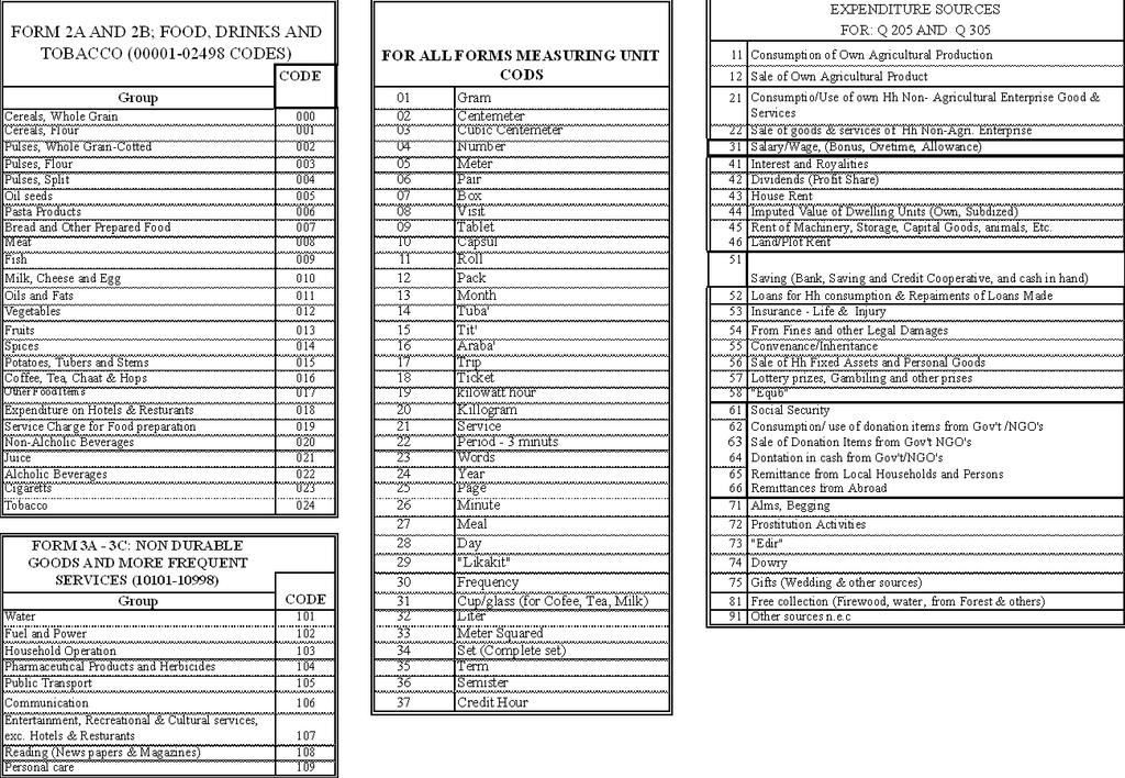
93

94

95

96

97

98

99

100

101