The Disposition Effect and Expectations as Reference Point

Transcription

1 The Disposition Effect and Expectations as Reference Point Juanjuan Meng 1 University of California, San Diego 23 January 2010 (Job Market Paper) Abstract: This paper proposes a model of reference-dependent preferences to explain the disposition effect, the tendency for investors in the stock market to be more willing to sell winners than losers. Focusing on aversion to losses relative to a reference point, the model predicts a V-shaped relationship between the optimal stock position and capital gains, which closely links the bottom point of the V shape to the reference point. I estimate the model empirically using Odean (1999) s data on individual trading from a large brokerage house. The estimates show that (i) the predicted V-shape relationship exists for a large majority of investors, and (ii) the estimated reference point demonstrates properties that make expectations the most reasonable candidate. The fact that reference point is influenced by expectations that are mostly positive due to the initial purchase decision allows a simple explanation of the disposition effect. Keywords: the disposition effect, prospect theory, loss aversion, expectations as reference point, threshold model. 1 Department of Economics, University of California, San Diego Gilman Drive, La Jolla, CA, jumeng@ucsd.edu. I am grateful to Terrence Odean for generously sharing the data with me. I want to give special thanks to my advisor Vincent Crawford for his insightful guidance and generous support. I also thank Nageeb Ali, Yan Bao, Nicholas Barberis, Dan Benjamin, Julie Cullen, Gordon Dahl, Stefano Dellavigna, David Eil, Uri Gneezy, Xing Huang, Botond Kőszegi, Ulrike Malmendier, Jian Li, Matthew Rabin, David Miller, Justin Rao, Joel Sobel, Changcheng Song, Yixiao Sun, Richard Thaler, Allan Timmermann and seminar audiences at UCSD for their helpful comments and suggestions. 1

2 1. Introduction The disposition effect refers to the observation that stock market investors tend to hold on to their losers for too long and sell their winners too soon, with losers and winners defined by comparing current price to the initial or (when a stock s shares were acquired at different times) the average purchase price (Shefrin and Statman 1985; Odean 1998; Weber and Camerer 1998). 2 Odean (1998), for instance, analyzes trading records of individual investors at a large discount brokerage house. He finds strong asymmetry between sale probabilities of stocks that currently show a gain and a loss relative to the average purchase price. He considers explanations for this asymmetry based on a neoclassical expected-utility model, finding that explanations from portfolio balancing, transaction costs, taxes, or rationally anticipated mean reversals can be excluded by the data. Weber and Camerer (1998) replicate the disposition effect in the lab, finding that incorrect beliefs of mean reversals cannot explain the phenomenon either. 3 Similar phenomena have been documented in other investment settings (Health, Huddart and Lang 1999; Genesove and Mayer 2001; Coval and Tyler 2005). The disposition effect poses a theoretical challenge to explanations based on expected-utility maximizing investors, in that there is no reason why the sharp changes in risk aversion needed to explain the disposition effect should occur around the initial or average purchase price, especially when investors have varying wealth levels, different starting positions on stocks and distinct purchase prices. The most popular informal explanation for the disposition effect has been prospect theory (Kahneman and Tversky 1979; Odean 1998). 4 Prospect theory assumes that the carrier of utility is not the level of wealth, but the change in wealth relative to a reference point. The literature often treats the status quo as the reference point. In the setting considered here, this would imply treating zero capital gain as the reference level of capital gains, or equivalently, the purchase price as the reference level of price (e,g. Shefrin and Statman 1985; Kahneman, Knetsch and Thaler 1990; Benartzi and Thaler 1995; Genesove and Mayer 2001). Prospect theory has three main elements: loss aversion with respect to the reference point, diminishing sensitivity (concavity above and convexity below the reference point), 2 To keep it consistent with the previous literature, the rest of the paper continues with this definition of winners and losers when talking about empirical facts of the disposition effect, even though the true reference level of price may not be the initial or average purchase price. Odean (1998) shows empirically that results are not dependent on whether the initial purchase price or the average purchase price is treated as the reference level of price. 3 In Weber and Camerer (1998) s study, when forced to sell the losers and given chances to buy them back, most subjects refuse to do so. 4 Prospect theory generates individual trading behavior that in equilibrium can explain various puzzles in asset pricing: Benartzi and Thaler (1995) use prospect theory to explain the equity premium puzzle; Barberis, Huang and Santos (2001) show that prospect theory type of preferences, combined with changes in risk attitudes after prior gains and losses can generate high mean, high volatility, and cross-sectional predictability in returns. Brinblatt and Han (2005) suggest that the undervaluation of stocks after gains and overvaluation of stocks after losses generated by prospect theory can predict short-run momentum in returns if the distorted prices are corrected by rational investors. Coval and Tyler (2005) confirm Brinblatt and Han (2005) s model while studying the trading behavior of Chicago Board of Trade proprietary traders. 2

3 and nonlinear probability weighting. 5 For simplicity, this paper ignores nonlinear probability weighting. The informal explanations have so far focused on diminishing sensitivity: investors in the gains domain are more risk averse, so more likely to sell a stock (obtaining less risky cash in return); while investors in the losses domain are less risk averse, hence more willing to hold a stock. But loss aversion also influences attitudes toward risk in a way that has the potential to explain the disposition effect. When a investor s probability of crossing the reference point is nonnegligible, the kink associated with loss aversion causes first-order risk aversion (Rabin 2000), potentially decreasing the investor probability of holding a stock much more than any plausible effect of diminishing sensitivity. 6 Translating an explanation of the disposition effect based on prospect theory into a formal model has been challenging (Barberis and Xiong 2009; Hens and Vlcek 2005; Gomes 2005). Barberis and Xiong (henceforth BX ) (2009) propose a formal model of selling behavior based on both loss aversion and diminishing sensitivity, taking into account that investors rational expected returns should be positive to justify the initial purchase decision. They show that for a binomial returns distribution with a reasonable range of positive means, taking the status quo as the reference point, prospect theory in its original parameterization (Tversky and Kahneman 1992) actually generates the opposite of the disposition effect in most cases. 7 While diminishing sensitivity contributes to the disposition effect in BX s model, the unexpected result comes from loss aversion. Loss aversion tends to make investors choose gambles whose worst (or respectively best) outcomes leave them at or near the reference point. If the reference point is determined by the status quo, then zero capital gain is the reference level of capital gains (i.e. the purchase price is the reference level of price). A returns distribution with positive mean normally generates larger capital gains than capital losses (in absolute terms). So capital gains are on average farther from the reference level than capital losses. It therefore requires taking larger position on the stock with a capital gain for the worst outcome to be near the reference point than it takes on the stock with a capital loss for the best outcome to be near the reference point. 8 Loss aversion (even though partially offset by the effect of diminishing sensitivity) therefore generates more sales below than above zero capital gain. 5 Loss aversion refers to the fact that losses hurt people more than gains please them. It brings first-order effect to the preferences by introducing a kink at the reference point in the value function. Loss aversion has been widely supported by lab and empirical evidence (e.g. Kahneman, Knetsch and Thaler 1990; Sydnor 2008; Camerer et al 1997; Benartzi and Thaler 1995). Diminishing sensitivity assumes that people are less sensitive to changes of big gains and losses than small ones, while nonlinear probability weighting assumes that people systematically overweight small probabilities. 6 Decision makers exhibiting first-order risk aversion are risk averse to even very small gambles; while those with secondorder risk aversion, normally represented by the usual concave utility function, are risk neutral to small gambles. 7 Their original formulation takes the initial wealth (with interest earnings) as the reference point. It can be easily translated as the initial purchase price (with interest earnings) in price space. In section III of the paper BX also sketch a model based on realization utility that distinguishes between paper and realized gains and losses. Realization utility is capable of generating the disposition effect, and I will discuss this alternative in section 4. The analysis of this paper, however, still follows the traditional assumption not to distinguish between paper and realized gains/losses. 8 BX (2009) show this asymmetry with a binomial distribution, and confirm its robustness with a lognormal distribution. 3

4 Although BX carefully investigate the robustness of their results in several directions, they do not consider alternative specifications of the reference point. However, positive expected return and the associated asymmetric capital gains and capital losses realization around zero play a less important role for the disposition effect when the reference point is not closely tied to the status quo. The empirical literature on prospect theory has taken equivocal positions on what determines reference points. Although the early literature (e,g. Shefrin and Statman 1985; Kahneman, Knetsch and Thaler 1990; Benartzi and Thaler 1995; Genesove and Mayer 2001) assumes that the reference point is the status quo, Kahneman and Tversky (1979) also note that there are situations in which gains and losses are coded relative to an expectation or aspiration level that differs from the status quo. Kőszegi and Rabin (2006, 2007, 2009) develop this idea in their new reference-dependent model by endogenizing the reference point as lagged rational expectations. This paper reconsiders the possibility of explaining the disposition effect via loss aversion, taking a broader view of the reference point. I model the investors decision problem much as BX (2009) do, but with differences in the following aspects: First, I assume loss aversion but not diminishing sensitivity. Since diminishing sensitivity has explanatory power for the disposition effect, ignoring it strengthens my main point, that prospect theory can provide a credible explanation for the disposition effect. Second, I generalize returns distribution from BX s binomial or lognormal to any continuous distribution, so that the model shows a complete picture of the non-monotonic changes in risk attitudes caused by loss aversion. For any exogenous and deterministic reference point, my model predicts a V-shaped relationship between the optimal position on stock and current capital gains, with the bottom point of the V shape closely linked to the reference point. BX (2009) and Gomes (2005) analyze the implications of this V-shaped relationship with binomial returns distribution under the assumption that the reference point is determined by the status quo. This paper explicitly establishes this relationship for any distribution and any exogenous and deterministic reference point. The characterization of this relationship also provides a reasonable empirical strategy that enables me to infer where the reference point is from the data. I further show that if the reference point is determined by expectations, which the initial purchase decision suggests are positive, then loss aversion alone, without diminishing sensitivity, can generate the disposition effect. The intuition is the following: First-order risk aversion caused by loss aversion suggests that the closer capital gains are to the reference level, the more risk-averse investors are, and the more likely they are going to sell the stocks. If the reference level of capital gains is determined by positive expectations, most capital gains are closer to the reference level than most capital losses. Investors are therefore more likely to sell when stock prices appreciate from the average purchase price. This argument is able to get around BX s results because of the disentanglement of the reference point from the status quo. Give expectations as the reference point, although most capital gains are still farther away from zero than most capital losses, capital gains are actually closer to the reference level. 4

5 As the major result of the model, the V-shaped relationship implies the disposition effect, but it is a stronger testable prediction. (For instance, a threshold strategy of selling the stocks once certain positive capital gains threshold is reached is also capable of generating the disposition effect, but will not yield a V-shaped relationship.) In the empirical analysis, I document a novel non-monotonic and largely V-shaped relationship between the probability of holding stocks and current capital gains, using individual trading records from a large brokerage house used by Odean (1999) and Barber and Odean (2000,2001). 9 Several papers have partially characterized the implications of this relationship using various data sets (Odean 1998; Grinblatt and Keloharju 2001; Ivković, Poterba and Weisbenner 2005). 10 This paper is the first to document and analyze the complete quantitative pattern, which confirms the prediction of loss aversion. This paper also contributes empirical evidence to support the new referencedependent model developed by Kőszegi and Rabin (2006) that treats expectations as the reference point. 11 My estimates of the aggregate sample suggest that investors reference points are most likely affected by expectations. The bottom of the V shape is estimated to be at 5.5% capital gain, which reflects the average reference level of capital gains across investors. Qualitatively, investors expected capital gains should be strictly positive to justify their initial purchase decision, and the estimated 5.5% is significantly different from zero. Quantitatively, expected capital gains should be related to the market returns. For the average holding period in the sample, the market return is 4.8% five years prior to the sample period, and 5.9% during the sample period, both very close to the 5.5% estimate. My estimates of the heterogeneity in the sample provide further evidence to support expectations as the reference point. The first heterogeneity lies in the probability of holding stocks between frequent traders and infrequent traders. I model the difference of trader type by the difference in time horizon to evaluate gains and losses. Due to short holding period frequent traders expect lower capital gains given positive expected returns. If the reference level is affected by expected capital gains, then the model predicts a lower bottom point of the V shape for frequent traders. The estimation shows that the bottom 9 Odean generously shared his data with me. 10 Using an individual trading data set different from the one used in this paper, Odean (1998) shows that investors are more likely to hold big winners and losers than small ones. Grinblatt and Keloharju (2001) find the same tendency with losers using trading records of Finnish investors. Working with the same data set as this paper, Ivković, Poterba and Weisbenner (2005) find that the relationship between the probability of holding stocks and capital gains is negative within six months after purchase, and positive after twelve months, which is related to the implications of the V-shaped relationship between the probability of holding stocks and current capital gains. 11 Several empirical papers have tested Kőszegi and Rabin s assumption that reference points are determined by expectations. In a lab experiment, Abeler, Falk, Goette, and Huffman (forthcoming) show directly that subjects labor supply decision is determined by reference point defined by expectations rather than the status quo. Ericson and Fuster (2009) manipulate the trading opportunity in an exchange setting and suggest that subjects behavior is driven mainly by expectations but not status quo. Gill and Prowse (2009) show in a real effort competition setting that agents respond negatively to their rivals efforts, a prediction from disappointment aversion that treats the certainty equivalent of the lottery a plausible proxy for expectations as the reference point. In field setting, Crawford and Meng (2009) treat reference points as expectations, proxy them by natural sample averages, and show that a reference-dependent model with such reference points provides a useful account of cabdrivers labor supply behavior. Card and Dahl (2009) s empirical analysis suggests that emotional cues generated by unexpected losses by the home team increase family violence. 5

6 point of the V shape is indeed lower for frequent traders (1.8%) than infrequent traders (10.3%). Since frequent traders hold the stocks for only a short period, they are also less likely to adjust the expected capital gains too widely from the initial levels. Thus in aggregation the relationship between the probability of holding stocks and current capital gains should match the V shape prediction derived from the model with a fixed reference level of capital gains pretty well. At the same time since infrequent traders are more likely to adjust their expected capital gains widely due to longer holding period, the aggregate pattern may not be strictly V-shaped. This prediction is confirmed by the data. The second heterogeneity comes from the probability of holding stocks between stocks with increasing prices and those with decreasing prices during the holding period. Expected capital gains are based on both the realization of capital gains during the period of holding and future expected returns. In the absence of changes in beliefs about future returns, investors should expect higher capital gains for stocks with increasing prices between the purchase date and current date, simply because good price history endows them with higher expected capital gains to start with. Therefore after controlling for beliefs changes, the estimated bottom point of the V shape should be higher for stocks with increasing price history than those with decreasing price history. This prediction is also consistent with the pattern in the data: Among frequent traders the bottom point of the V shape is 1.8% for stocks with increasing price history, and it is 0.7% for stocks with decreasing price history. Among infrequent traders, the estimated bottom of the V shape occurs at 11.9% for stocks with increasing price history and 0.9% for stocks with decreasing price history. In summary, this paper shows that for a general returns distribution with positive expected return, loss aversion with reference point defined by expectations reliably implies a disposition effect of the kind commonly observed. Diminishing sensitivity reinforces the disposition effect, but it is not essential for a satisfactory explanation. As far as I know, this paper is the first to completely document a largely V-shaped relationship between the probability of holding stocks and capital gains. Such relationship confirms the existence of loss aversion. This paper is also the first to estimate the reference point from individual trading data. The estimation results support the recent theoretical development that treats expectations as the reference point. The rest of the paper is organized as follows. Section 2 proposes a simple static reference-dependent model that generates the V-shaped relationship. Section 3 uses Odean (1999) s individual trading data to estimate the relationship between the probability of holding stocks and capital gains. Section 4 discusses a promising alternative theory of investors selling behavior based on realized gains or losses proposed by BX (2008, 2009 Section III). I then conclude the paper. 2. The Theoretical Model 2.1 Set-up 6

7 The model looks at a static wealth allocation problem in which an investor has to decide how to split her wealth between a risky asset (stock) and cash. For simplicity I assume no short selling, no time discounting, and no return and inflation risk on cash. The net return of the stock each period is u t, which is independently and identically distributed with a continuous distribution on the support ( 1,+ ). The investor starts with a given initial wealth W 0 out of which is allocated to the stock, and to cash, where is the number of shares, and is the purchase price. I treat the initial position as given here, but as Barberis and Xiong (2009) and Hens and Vlcek (2005) suggested, I take into account the restriction on beliefs about returns implied by the initial purchase decision by imposing positive expected return. 12 Section 2.3 discusses the implications of including the initial decision into the analysis. In period one, P 1 = P 0 (1+ u 1 ) is realized. The capital gains in period one are defined as r 1 = (P 1 P 1 ) /P 1 = (P 1 P 0 ) /P 0 = u 1, where P 1 is the average purchase price before making period one decision, which is simply the initial purchase price P 0. The investor then chooses a stock position x 1 to maximize the gain-loss utility in period two. In period two, P 2 = P 1 (1+ u 2 ) is realized. The investor incurs the gain-loss utility over changes in wealth relative to a reference point. 13 The decision problem is to choose the optimal stock position x 1 * in period one to maximize the following utility incurred in period two: E(U(W 2 W 1,2 RP )) = E(1 {W2 W 1,2 RP >0} (W 2 W 1,2 RP ) + λ1 {W2 W 1,2 RP 0} (W 2 W 1,2 RP )) (1) subject to the budget constraint 0 x 1 P 1 B 0 + x 0 P Where W 2 = B 0 + P 1 (x 0 x 1 ) + P 2 x 1 (2) 12 If the investor considers portfolio choice, then she may accept negative expected return granted that this stock is negatively correlated with some other stocks in the portfolio. However, Barberis and Huang (2001) show that most investors exhibit narrow framing by making decision at individual stock level. Even if portfolio concern is present, investors should still accept only positive expected returns for majority of the stocks in the portfolio so that this assumption still applies to most cases. 13 Following BX (2009), this paper does not consider consumption choice and defines utility directly over wealth. It can be understood as an implicit function approach that reflects utility from an optimal consumption plan in the future given certain wealth level today. Kőszegi and Rabin (2009) assume that people incur anticipatory utility from expectations of future consumption. Thus utility generated by wealth fluctuation compared to the reference point can be motivated by changes in expectations about future consumption plan, a concept called prospective gain-loss utility in their model. 14 Kőszegi and Rabin (2006) develop a more general version of the reference-dependent preferences by treating total utility as a weighted average of the consumption utility and gain-loss utility, where the unit for gain-loss comparison is also the consumption utility: RP E(V(W 2 W 1,2 )) = E(U(W2 ) + η(1 (U(W ) U(W RP {W2 W RP 1, 2 >0} 2 1,2 )) + λ1{w2 (U(W ) U(W RP W1, RP 2 0} 2 1,2 )))). is the traditional consumption utility, and is the weight attached to the gain-loss utility. This more general version keeps the essentials of loss aversion while incorporating the effect of standard consumption utility. My model therefore can be viewed as a simplified version in which the consumption utility is linear. Having a concave consumption utility function does not change the V shape, but it shifts the bottom of the V shape away from the reference point. 7

8 W 1,2 RP = B 0 + x 0 P 0 (1+ r 1,2 RP ) (3) W 2 is the wealth level in period two. W RP 1,2 is an exogenous and deterministic reference point that the investor holds in period one about the wealth level in period two. Although the reference point is defined over wealth, I assume that it is determined by r RP 1,2, the reference level of capital gains. Thus r RP 1,2 will be the primary focus in the discussion of the paper. r RP 1,2 is different from the return of a single period u t because the former is calculated from comparing price in period two to the average purchase price, which is simply P 0 in period one. W RP 1,2 is exogenous in the sense that it does not incorporate the effect of the position x 1 taken in period one. Based on r RP 1,2 one can also calculate the corresponding reference level of price P RP 1,2 = P 0 (1+ r RP 1,2 ) as the price level in period one at which the investor can simply sell the entire stock position and reach the reference point in period two. 1 {W2 is an indicator representing a loss, which takes the value one if W RP 1,2 0} the condition W 2 W RP 1,2 0 is satisfied, otherwise zero. If wealth in period two falls below the reference point, the difference is multiplied by, representing loss aversion. Since I do not assume diminishing sensitivity, the utility function is piece-wise linear. The kink at the reference point characteristic of loss aversion is thus the only source of risk aversion. The literature on reference-dependent preferences and the disposition effect normally takes the status quo as the reference point. 15 In the current setting, the status quo is the initial wealth W 0, which comes from r RP 1,2 = 0, or equivalently P RP 1,2 = P 0 (Shefrin and Statman 1985; Odean 1998). This paper proposes expected wealth W E 1,2 = B 0 + x 0 P 0 (1+ u 1 )E(1+ u 2 ) as an alternative reference point. It reflects the mean expectations the investor forms about the period two wealth before making period one choice. Such reference point comes from expected capital gain as the reference level of capital gains (r E 1,2 = (1+ u 1 )E(1+ u 2 ) 1), or equivalently the expected price as the reference level of price (P E 1,2 = P 0 (1+ u 1 )E(1+ u 2 )). 16 Finally, the assumption of positive expected return directly implies E(r E 1,2 ) > 0, i.e. in most cases the expected capital gain is positive. Following BX, my model makes a non-trivial assumption of narrow framing or mental accounting (Thaler 1990). First, the model assumes that the investor incurs gain- 15 With the exception of Health, Huddart and Lang (1999), where they look at the exercise of options so there is no purchase price to rely on. They basically show that recent historical-high price is a big driver of the exercise decision. 16 Kőszegi and Rabin (2006) model reference point as the whole distribution of lagged stochastic expectations, in which they assume that the reference point should be the optimal solution given the reference-dependent preferences based on it (the personal equilibrium ), and the reference point is slow in taking current resolved uncertainty into account. The simple definition of expected wealth given here does not satisfy the concept of personal equilibrium, and I do not assume lagged adjustment. For the purpose of explaining the disposition effect and distinguish between the status quo and expectations as the reference point, these theoretical properties are not necessary. Therefore I intentionally keep the specification of expectations simple. However, other ways of modeling expectations can also generate the disposition effect, as long as they reflect its positive nature. 8

9 loss utility at the individual stock level rather than the portfolio level. Correspondingly, W 0 can be viewed as the maximum amount of money that the investor is willing to lose on a particular stock (Barberis, Huang and Thaler 2006; Barberis and Xiong 2009). Barberis and Huang (2001) show that treating trading decisions as if investors were considering each stock separately fits the data better than including portfolio choice. Odean (1998) also shows that the disposition effect cannot be explained by portfolio concern. Second, the model assumes that the investor evaluates her investment outcomes and incurs gain-loss utility over a certain narrow period. Benartzi and Thaler (1995) call it myopic loss aversion and estimate the time frame to be one year from the aggregate stock returns. My model can therefore be viewed as describing optimal decision within one such evaluation period. I do not take a position on what the reference point is when solving the model. Instead I derive the model s predictions for any exogenous and deterministic reference point, in preparation for Section 3 s econometric analysis, where the model will be used to infer its location from the patterns in the data. 2.2 Solution To make it consistent with the empirical analysis, I discuss the optimal position for each level of capital gains. Since r 1 is a monotonic transformation of price P 1, the same solution holds in price space. In period one, loss aversion introduces a cut-off point that divides future return u 2 into gains and losses relative to the reference point, which are assigned weight 1 and λ >1 respectively. Given the exogenous reference level of capital gains r RP 1,2 and the current capital gains r 1, the cut-off point K(x 1 ) = x 0 ( 1+ r 1,2 1) is a x 1 1+ r 1 function of the current position x 1. K(x 1 ) is a specific level of u 2 that makes period two wealth equal to the reference point(w 2 = W RP 1,2 ). Equation (4) gives the expected marginal utility of holding an additional share. + K(x 1 ) E(MU(K(x 1 ))) = P 1 ( u 2 f (u 2 )du 2 + λu 2 f (u 2 )du 2 ) (4) K(x 1 ) 1 The optimal solution x * 1 satisfies the first-order condition E(MU(K(x * 1 ))) = 0. Under the piece-wise linear assumption, the choice variable x 1 enters the first-order condition only through the cut-off point K(x 1 ). 17 So x * 1 can be derived from the specific value of the cut-off point that satisfies the first-order condition. Proposition 1 gives the solution. RP 17 The expected marginal utility also includes the effect of the changes in x 1 to the cut-off point K (x 1 ), but this term is zero by the fact that at the return level of K (x 1 ), future wealth level equals its reference point W 2 = W 1,2 RP, so marginal changes in K (x 1 ) brings almost no changes to the expected gain-loss utility. 9

10 Proposition 1. For each returns distribution f (u t ) satisfying E(u t ) > 0 and E(MU(K(x 1 ) = 0)) < 0, there exist two deterministic return levels K 1 < 0 and K 2 > 0 that satisfy E(MU(K 1 )) = E(MU(K 2 )) = 0. The optimal interior position is given by x 0 ( 1+ r RP 1,2 RP 1), for r 1 < r 1,2 K 2 1+ r 1 x x * 1 = 0 ( 1+ r RP 1,2 RP 1), for r 1 > r 1,2 K 1 1+ r 1 RP 0, for r 1 = r 1,2 The budget constraint binds for extremely high or low capital gains r 1. The restrictions on the returns distribution mean that the returns should be good enough to attract purchase in the first place ( E(u t ) > 0), and they should not be too lucrative to make even a investor with loss aversion never want to sell the stock ( E(MU(K(x 1 ) = 0)) < 0). Since the investor assigns any return below the reference point a higher weight, and any negative return brings negative marginal utility, the expected marginal utility is decreasing in K(x 1 ) whenk(x 1 ) < 0. Similarly, since any positive return brings positive marginal utility, the expected marginal utility is increasing in K(x 1 ) when K(x 1 ) 0. When r 1 < r 1,2 RP, K(x 1 ) (0,+ ) as x 1 varies within the budget constraint. As K(x 1 ) goes to zero, by assumption the expected marginal utility is negative. As K(x 1 ) goes to positive infinity, all the returns are in the losses domain hence weighted equally by loss aversion coefficient λ, so the expected marginal utility is positive because of the positive expected return. Since the expected marginal utility is decreasing in K(x 1 ) in this region, there exists a cut-off point K 2 > 0 such that the expected marginal utility is zero. Given a specific returns distribution, the value of K 2 is fixed, so the optimal position for each current price r 1 < r 1,2 RP is determined by K(x 1 * ) = K 2. When r 1 > r 1,2 RP, K(x 1 ) (,0) as x 1 varies within the budget constraint. As K(x 1 ) goes to negative infinity, all the returns are in the gains domain and weighted equally so the expected marginal utility is again positive. Since expected marginal utility is decreasing in K(x 1 ) in this region, there exists another cut-off point K 1 < 0 that satisfies the first-order condition. Hence the optimal position for each current price r 1 > r 1,2 RP is determined by K(x 1 * ) = K 1. When r 1 = r 1,2 RP, K(x 1 ) = 0. The investor demands zero share of the stock because of the negative expected marginal utility. With a binomial distribution, BX (2009) show that it is optimal for investors to gamble until the highest (lowest) wealth reaches the reference point if currently in the losses (gains) domain. Proposition 1 confirms and generalizes this conclusion with any continuous returns distribution, by showing that investors will gamble until the wealth (5) 10

11 generated by a fixed return reaches the reference point when currently in the losses domain, or until the wealth generated by a fixed cut-off return reaches the reference point when currently in the gains domain. The intuition is the following: Being in the losses domain makes the investor willing to take more risks in order to go back to the reference point. However, she needs to limit her risk exposure to avoid incurring huge future losses. Therefore she prefers to take a position so that only the returns higher than are counted as gains. Similarly, if the investor is currently in the gains domain, she feels that she can afford taking more risks as long as the probability of falling below the reference point is low. So she is willing to accept a position that only makes returns lower than K 1 counted as losses. Given the strategy for the cut-off returns to reach the reference point, it is easy to understand how the optimal position changes with different capital gains in period one. Corollary 1 gives a more intuitive account of the relationship. Corollary 1: For the optimal positions that are interior, (i) decreases in r 1 when r 1 < r 1,2 RP, and increases in r 1 when r 1 > r 1,2 RP. (ii) is concave in r 1 when r 1 < r 1,2 RP, and convex in r 1 when r 1 > r 1,2 RP. Point (i) in Corollary 1 simply suggests that different levels of r 1 generate different distances from the reference level r 1,2 RP. The closer r 1 is to the reference level r 1,2 RP, the more risk averse the investor is. So she takes minimum risks by demanding few shares of the stock when r 1 is close to r 1,2 RP, and takes more risks by increasing the position on the stock as r 1 deviates from r 1,2 RP. These facts bring a V-shaped relationship between the optimal position x 1 * and capital gains r 1, with the bottom of the V shape reached at r 1 = r 1,2 RP. Such relationship comes from both loss aversion and the monotonic probability of crossing the reference point as the position becomes larger. The optimal position x 1 * is concave when r 1 < r 1,2 RP and convex when r 1 > r 1,2 RP because the absolute value of the first derivative is always decreasing in r 1 but the sign changes around the reference level due to different signs of K 1 and K 2. Intuitively, it always takes a smaller position on stock with higher current price (hence higher capital gain) to narrow the distance between period two wealth and the reference point. So the increase in the optimal position is exacerbated (mitigated) as capital gains become smaller (larger). Figure 1 illustrates the V-shaped relationship. I show region where budget constraint does not bind. The optimal position reaches its minimum with a kink at r 1 = r 1,2 RP. This kink 11

12 comes from the different cut-off points used below and above the reference level. It is clear that the investor is most likely to sell the stock around r 1,2 RP, given a fixed. 18 Figure 1: The V-shaped relationship between the optimal position and current capital gains for any exogenous and deterministic reference point. For r 1 of equal distance from the reference level r 1,2 RP, whether the high capital gains or the low ones lead to higher x 1 * is ambiguous. 19 However, the asymmetry in x 1 * around r 1,2 RP, if any, is less relevant in explaining the disposition effect once r 1,2 RP is different from zero (i.e. the reference level of price is different from the average purchase price). Since the disposition effect describes asymmetric behavior around zero capital gain, it is this asymmetry, not the asymmetry around the reference level of capital gains r 1,2 RP, in which we have interest. With the V-shaped relationship, it is convenient to illustrate both BX s argument for why prospect theory fails to predict the disposition effect when zero capital gain (i.e. the average purchase price) is treated as the reference level (figure 2) and how assuming positive expected capital gain as the reference level generates the disposition effect (figure 3). 18 The comparative statics analysis with respect to the loss aversion coefficient λ and the returns distribution f (u t ) delivers a more complete picture of the model. Both affect the optimal position through the optimal cut-off points K 1 and * K 2. An increase in λ leads to lower x 1 for every level of capital gain. Loss aversion, like conventional risk aversion, reduces investment demand for the risky asset. In terms of returns distribution, any move of probability mass from negative returns to positive returns will increase the position on stocks at all levels of capital gain, but still keep the V- shaped relationship unchanged. 19 In the current setting it mostly depends on where the cut-off points K 1 and K 2 stand relative to zero, which in turns depends on the returns distribution. For example, any returns distribution with an increasing f (u t ) in the region u t [K 1,K 2 ] implies K 1 > K 2, leading to relatively smaller position on the stock above the reference level. 12

13 Figure 2: The V-shaped relationship between the optimal position and current capital gains when reference point is status quo. Figure 3: The V-shaped relationship between the optimal position and current capital gains when the reference point is expectations. In figure 2 BX s argument relies crucially on the reference level of capital gains being zero ( r RP 1,2 = 0). Under returns distribution with positive mean, a representative realization of capital gains r G 1 will be relatively farther away from zero compared to a representative realization of capital loss r L 1. It therefore takes a larger position for future wealth generated by cut-off return to reach the reference point in the case of capital gains. Diminishing sensitivity in BX s model mitigates this tendency in favor of the disposition effect but is not enough to totally offset it. 13

14 This paper generates the disposition effect without relying on diminishing sensitivity because of the disentanglement of the reference level of capital gains from zero. Figure 3 illustrates the case when the reference level is affected by expected capital gain r 1,2 E, which is strictly positive in most cases. Due to the shift of the reference level from zero to a positive level, capital gains are on average closer to zero than capital losses. Because the investor is most likely to sell around the reference level of capital gains due to loss aversion, she is more likely to sell the stock when it has a capital gain than when it has a capital loss. So far the model s predictions are derived under a given initial purchase decision. However, the initial decision is potentially important because incorporating it makes BX to argue that prospect theory generates the opposite of the disposition effect when the status quo is the reference point. If the reference point is determined by expectations, then investors are willing to accept lower returns than in BX s model. It implies two things: First, it makes the disposition effect weaker because the reference level of capital gains is closer to zero for stocks purchased. But because investors should still accept only positive returns, the disposition effect will still be present. Second, lower expected returns reduce the asymmetry in the realization of capital gains around zero, which favors the disposition effect. In general, incorporating the initial decision when reference point is affected by positive expected capital gain should not change the major prediction of the model. 2.3 Robustness My simple model predicts a V-shaped relationship between the optimal stock position and capital gains, which is sufficient but not necessary to generate the disposition effect. The model also implies that the bottom of the V shape is reached when r 1 = r 1,2 RP. In this section I discuss the robustness of these results. The V-shaped relationship is relatively robust, but not to endogeneity of the reference point, or multiple reference points. Under more general conditions, the bottom of the V shape may not be reached at its reference level. However, the bottom of the V shape is largely driven by the reference level of capital gains thus still provides valuable information about its qualitative properties. Diminishing sensitivity: Making the value function concavity above and convexity below the reference point as Tversky and Kahneman (1992) estimate them keeps the V- shaped relationship, because diminishing sensitivity itself generates monotonically decreasing stock position. The bottom of the V shape, however, is not exactly at its reference level, instead it is pushed slightly to the right of its reference level (Barberis and Xiong 2009; Gome 2005). Since the value function with diminishing sensitivity is not globally concave, there is a discontinuous decline in the optimal stock position at the bottom of the V shape (Gomes 2005), partially reflecting the power of diminishing sensitivity to explain the disposition effect. Multiple periods: In a reasonable extension of the model the investor should have many decision periods before she evaluates the gain-loss utility. The future independent risks in returns will partially cancel each other and make the investor demand more shares in the current period. This dynamic effect affects the level of the optimal position, but does not affect the qualitative nature of the V-shaped relationship. The bottom of the V shape is 14

15 still the reference point. The dynamic aspect has additional impact if the future reference point is affected by current holdings. In this case the sophisticated investor will take into account this effect when making her current allocation decision. Since there is a tendency to keep the future reference point low to avoid sensations of big losses, if a larger position on the risky asset leads to high reference point in the future then the sophisticated investor will take smaller position today, again affecting the level of the optimal position but not the V-shaped relationship. 20 Endogeneity of the reference point: If the current reference point is strongly affected by the current position, then the optimal position may not be V-shaped any more. 21 The reason is that endogenous reference point generally moves with current position and price, moving K 1 and K 2 as well. Without a fixed cut-off point, it does not necessarily take a larger position to achieve optimality as capital gains deviate from the reference level. It is interesting to testing the predictions of endogenous reference point, but given a strong V- shaped pattern in the data, it seems more natural to explore the possibilities of models that explain this pattern with exogenous reference point. Two reference points: The investor may incur gain-loss utility compared to different reference points, and the total utility is a weighted average of them. For instance, she may compare outcomes to both the initial wealth and the expected wealth. Appendix A analyzes this case in details. Depending on the returns distribution f (u t ), there are two possible patterns. Under the single-trough pattern the optimal position is still V-shaped but the bottom of the V shape is located between the two reference levels of capital gains. Under the twin-trough pattern the optimal position is W-shaped, with a local minimum position at each reference level. My model predicts that for a consistent investor who believes that the returns distribution is independently and identically distributed, if the reference level of capital gains is zero, which does not change over time, then once she purchases the stock she will never wants to sell. This theoretical reasoning makes it unlikely for the status quo to be the reference point. The problem of never wanting to sell does not exist under additional assumptions such as diminishing sensitivity and multiple reference points, because they permit shift of the bottom of the V shape away from the reference point. However, the empirical analysis does not impose the theoretical structure on estimation, i.e. my econometric model is free to pick up zero as the reference level of capital gains, if data suggests so. If we indeed estimate a bottom point of the V shape at zero capital gain, then we need to modify the model to address this problem. However, given that this is not happening in the data, the problem seems to be minor. 20 Discussion of such effect is included in the dynamic reference-dependent model developed by Kőszegi and Rabin (2009). 21 There are several examples of such endogenous reference point in the literature. For instance, in the disappointment aversion literature, the reference point is the certainty equivalent of the lottery generated by the action. In Kőszegi and Rabin (2006) s personal equilibrium the reference point is the distribution of outcomes generated by the contingent action plan before uncertainty is resolved. 15

16 3. Empirical Analysis This section tests the V-shaped relationship between the optimal position and capital gains by looking at individual trading behavior in the stock market. The data set is from a large discount brokerage firm on the investments of 78,000 households from January 1991 through December The data set was used by Odean (1999) and Barber and Odean (2000,2001). It is different from the one that Odean (1998) used in his pioneering analysis of the disposition effect. In the individual trading records constructed from my data, only 4% of the observations are partial sales or repurchases. Most of the times investors sell either all or none of their positions in a given period. I therefore can proxy the optimal position with a binary hold variable ( if sell, and otherwise). Capital gains are denoted by, where P ijt and P ijt are the stock price and the average purchase price for account, stock, and time respectively. 22 Because of the binary nature of decision in the data, takes constant values at the initial purchase price most of the time. 3.1 The Data The data set includes end-of-month position statements, trading records (trade date, trade quantity, trade price) for each stock held by each account, as well as some background information about the account owners (e.g. gender, age, income, net wealth). I also have data for the daily stock price, daily trading volume, outstanding shares, an adjustment factor for splits and dividends and market returns (S&P) from CRSP. Odean (1999) gives more descriptions of this data set. Appendix B gives details of my data cleaning process. In this study I focus on trading of common stocks at the individual stock level, ignoring portfolio concern. My empirical analysis relies on constructing an investor s trading history for each stock. The history includes dates of purchases, holds and sales. Following Odean (1998) and Grinblatt and Keloharju (2001), I generate holding dates in the following way: any time that at least one sale takes place in the portfolio, I count the untraded stocks in the portfolio as holds, and obtain price information from CRSP for them. These are stocks that investors could have sold but did not. In other words, I select holding dates conditional on having at least one sale taking place in the portfolio on that day. This procedure is standard in the empirical literature of the disposition effect. This ensures that any holding decision in the sample comes from deliberation rather than inattention. For the purpose of studying the relationship between the optimal position and capital gains, it does not necessarily imply sample selection problem. However, there is some risk of bias if portfolio size and trading frequency are correlated to capital gains. I look at these possibilities later. 22 Note that is exactly one minus the sell dummy variable normally used in the literature, so the estimated coefficients have the opposite sign. For example, the bottom point of the V shape will be the point that investors are most likely to sell. 16

17 Table 1 reports the summary statistics of the dataset. All prices used to calculate capital gains are appropriately adjusted for commission, dividend and splits. 23 Table 1: Summary Statistics Mean Standard Deviations Min Max Observations Holding Days ,968 Realized Capital Gains ,968 Paper Capital Gains ,756 Portfolio Size ,128,724 Principal at the Initial Purchase 10,622 28, ,011, ,637 Commission per Share ,637 Income 95,851 3,728, ,671,000 36,174 Age ,724 I construct the variable trading frequency to be the inverse of the average time between two trades for each investor using the entire trading records, and assign investors with trading frequency higher (lower) than the mean as frequent (infrequent) traders. Frequent traders on average trade every month, and infrequent traders trade every five months. To measure the desirability of price history during the holding period, I calculate the proportion of increasing prices (compared to price of the previous observation) between the initial purchase date and the date in question, and assign observations with this ratio higher (lower) than the mean as having good (bad) history, in the sense that the stock price keeps going up (down) on average after purchase. 24 Stocks with good price history yield average capital gain of 22.4%, and stocks with bad price history yield average capital gain of -16.3%. For both sample splitting, ties are randomly assigned to each group. 23 Whether to adjust for commissions doesn t generate a big difference in the estimates. 24 I have tried other ways to assign an observation to have good or bad history, including constructing the proportion of positive capital gains and the proportion of positive market adjusted returns between the initial purchase date and the date in question. To check whether investors judge good or bad history more by recent returns, I also construct the proportion based on whether the average returns from the past week and past two months are positive or not. The qualitative results in the following discussion are robust to these alternative specifications. 17

18 Table 2: PLR and PGR Overall Sample Dec. Jan.-Nov. Frequent Traders Infrequent Traders Good History Bad History PGR PLR PLR-PGR t-statistic RG 184,802 11, ,930 37, , ,456 13,346 RG+PG 512,647 38, , , , ,519 61,128 RL 136,041 15, ,469 32, ,261 15, ,990 RL+PL 556,375 49, , , ,050 60, ,629 Note: This table calculates the proportion of gains realized (PGR) and the proportion of losses realized (PLR) following the strategy of Odean (1998 Table I). PGR is calculated by the number of realized capital gains divided by the number of realized and paper capital gains; PLR is calculated by the number of realized capital losses divided by the number of realized and paper capital losses. RG, PG, RL, PL represent numbers of realized capital gains, paper capital gains, realized capital losses and paper capital losses. The standard error is constructed by. I follow Odean s (1998) methods to analyze his (1999) dataset, and show that it does demonstrate the disposition effect, generating results qualitatively consistent with Odean s (1998) as well as Grinblatt and Keloharju s (2001). Odean (1998) count winners and losers relative to the average purchase price. 25 He defines the proportion of gains realized (hence PGR) as the number of realized capital gains divided by the number of realized and paper capital gains; and the proportion of losses realized (hence PLR) as the number of realized capital losses divided by the number of realized and paper capital losses. I count PGR and PLR the same as Odean (1998, table I) and report the results in table 2. In the overall sample, investors realize significantly more capital gains than losses, and the difference is large (PLR-PGR=-0.115). 26 In December the difference is not 25 A hold observation is counted as a gain (loss) if the lowest (highest) price of that day is higher (lower) than the average purchase price, respectively. 26 There is a quantitative difference between the current sample and Odean(1998) s. The difference between PLR and PGR is for the overall sample, higher than the in Odean (1998 table I). 18

19 significant, probably due to tax incentive to sell more losers than winners. 27 The difference between frequent and infrequent traders is also consistent with Odean s finding: although both types demonstrate the disposition effect, infrequent traders are especially vulnerable to this effect. 28 The distinction between good and bad history, which has not been investigated before, also reveals a surprising asymmetry: investors with good price history are more likely to sell their winners and hold on to their losers; the pattern is reversed when the price history is bad. I will show that loss aversion and expectations as the reference point provide a reasonable account of these observations. 3.2 The Overall Sample Analysis In this section I analyze the aggregate pattern, keeping the reference level of capital gains fixed across investors and estimate the location of the bottom of the V shape as a fixed number. Such analysis can be understood as referring to the trading pattern of the average investor. However, the homogeneity assumption is obviously too restrictive, especially when expectations are a candidate for the reference point. Section 3.3 partially relaxes this assumption by allowing heterogeneity along trading frequency and price history. The estimated relationship is largely consistent with the V shape predicted by the model. The bottom of the V shape is estimated to be at 5.5% capital gain for the overall sample, significantly different from zero, suggesting that treating the status quo as the reference point is not likely to be a very accurate assumption. Graphs Figure 4 shows the average binary holding decision for each 0.1 capital gains interval for the entire sample. It is the empirical analog of the V-shaped relationship derived in the theory section, and it can be understood as the sample probability of holding stocks at each capital gains interval. The relationship is clearly non-monotonic. Starting from -10% capital gain it is also V-shaped: in aggregate the probability of holding starts to decline from -10% to 10%, and then rises after 10%. The left-tail drop in the probability of holding is not predicted by my static model. Section 3.3 shows that it mainly comes from infrequent traders who face bad price history. I will propose possible explanations there. In the following discussion I focus on the region of capital gains larger than -10%. The important message from figure 4 is that the probability of holding reaches its minimum at a positive capital gain. This fact suggests that the reference level of price is affected by something higher than the average purchase price. Loss aversion combined 27 Because of tax on positive capital gains, it is often more beneficial for investors to realize capital losses than capital gains at the end of the year. Ivković, Poterba and Weisbenner (2005) identify the existence of tax-driven selling. 28 BX (2009) explain this fact by noting that infrequent traders have long holding period, so independent future risks can cancel each other and make investors more willing to accept stocks with lower expected returns today. Capital gains today are then distributed more symmetrically around zero, so their model is more likely to generate the disposition effect. 19

20 with diminishing sensitivity with the reference level of price at the average purchase price can in theory generate such positive bottom point of the V shape (Gomes 2005), but it cannot be an empirically plausible explanation because it fails to predict the disposition effect (Barberis and Xiong 2009). 29 Figure 4: the Probability of Holding Stocks Averaged at 0.1 Capital Gains Interval. Figure 4(S) graphs the same relationship in figure 4 but focuses on the capital gains range [-0.1,0.1], with the binary holding variable averaged for each capital gains interval. Although the bottom of the V shape is not reached at zero capital gain, there is a steep decline in the probability of holding stocks at zero. This pattern suggests that the role of the average purchase price is not negligible. My econometric model includes a dummy variable indicating positive capital gains to control for the effect of average purchase price If current model is viewed as a special case (with a linear consumption utility) of Kőszegi and Rabin (2006) s more general version of reference-dependent preferences that incorporates consumption utility, then a concave consumption utility can also shifts the bottom of the V shape away from the reference level. But similar to the case of the diminishing sensitivity, the magnitude of such shift is likely to be second-order hence too small to outweigh the asymmetric capital gains realization around zero given positive expected return. Furthermore, this explanation has a hard time accounting for variations in the bottom point of the V shape with trading frequency and price history (section 3.3). 30 The coexistence of a sharp decline in the probability of holding at zero capital gain and the bottom of the V shape at a positive capital gain can be understood better through a framework of two reference points. Appendix A analyzes this case in details. But two reference points are not essential to explain the disposition effect. It is also possible that investor 20

21 Figure 4(S): The Probability of Holding Stocks Averaged at Capital Gains Interval. Holding period, trading frequency, and portfolio size complicate the interpretation of figure 4, because they can be correlated with both the decision to hold stocks and capital gains. The following analysis confirms these possible correlations, but the general pattern in figure 4 is robust to the inclusion of these and more factors as controls, except that the drop in the probability of holding at the left tail is more severe with controls variables. Appendix D graphs the residuals of the probability of holding from a linear probability estimation that controls for additional factors. Holding period For each individual stock, holding period is the time between the initial purchase date and the date in question. It is positively correlated with the probability of holding a given stock in the sample, possibly because there is exogenous time preference for holding stocks. Holding period is also naturally related to capital gains, because the longer investors hold a stock, the wider range of capital gains they are likely to experience. If the type is heterogeneous, where one type has zero capital gain as the reference level, and another type has a positive capital gain as the reference level. However, in the subsamples by trading frequency and price history (section 3.3), the zero capital gain has significant influences over trading behavior in most cases. Even if there are different types it seems hard to find an intuitive criterion to sort them out. 21

22 relationship between holding period and capital gains is the same as the pattern in figure 4, then loss aversion may not be a valid explanation for the observed V shape. Figure 5A shows the average holding period at each 0.1 capital gains interval. The relationship is V-shaped, probably partially driving the pattern in figure 4. But holding period is symmetric around zero capital gain rather than a positive capital gain, so it is not likely to drive the specific pattern observed in figure 4. Figure 5A: The Average Holding Period. Figure 5B: The Average Trading Frequency. Figure 5C: The Average Portfolio Size. Trading frequency In the sample, trading frequency is strongly and positively correlated with the probability of holding stocks. This seeming counter-intuitive result comes from the sample selection procedure. In the sample infrequent traders are more likely to sell many stocks on a given day, so there are relatively fewer observations of holding decision being selected into the sample, lowering the probability of holding in the sample. If they realize 22

23 mostly small positive capital gains during their holding period, then the V shape looks like, but has nothing to do with loss aversion with respect to a positive reference point. Figure 5B graphs trading frequency against capital gains. Infrequent traders (with low trading frequency) are associated with large capital gains and losses, and the pattern is totally symmetric around zero. This relationship thus strengthens the V-shaped pattern in figure 4 because the sample selection procedure makes the probability of holding stocks higher at small positive capital gains, and makes it lower for big capital gains and losses. Portfolio size: Since I select dates of holding decision conditional on at least one sale taking place in the portfolio, portfolios with relatively fewer numbers of stocks bring fewer observations of a holding decision to the sample, lowering the sample probability of holding stocks. If stocks in the small portfolio have mostly small positive capital gains, then even when investors are equally likely to sell winners and losers, the sample selection leads to relatively low probability of holding stocks at small positive capital gains. Figure 5C graphs the average portfolio size at each 0.1 capital gains interval. There is indeed a tendency for small portfolios to have small positive capital gains, and the overall pattern looks similar to figure 4. However, a closer look suggests some quantitative differences: the bottom of the V shape occurs roughly at 10% in figure 4, whereas the smallest portfolio size is at zero in figure 5C. The left-tail slope change in figure 4 occurs at -10% but the similar left-tail change is at -30% in figure 5C. In general, portfolio size is an important factor to control for when estimating any causal relationship of capital gains on the probability of holding. However, it is not likely to create the specific patterns in the non-monotonic relationship seen in figure 4. Estimation Now I formally estimate the non-monotonic relationship in figure 4 using a multithreshold model with unknown thresholds (Andrews 1993; Bai 1996; Hansen 2000 a, b). A formal estimation is intended to check the robustness of the graphic relationship to the inclusion of more control variables, and to obtain accurate estimates of the bottom point of the V shape. A threshold model allows all or some of the coefficients to change at the threshold. Because the bottom of the V shape reflects a slope change that generates continuous adjustment around the change point, my econometric model restricts threshold as the slope change point to pick up the bottom of the V shape. The reason to allow for multiple thresholds is the observation from figure 4 that besides slope change at the bottom of the V shape there is also an obvious slope change at a small capital loss. Note that the threshold is not necessarily the reference level of capital gains: even the most important threshold, the bottom of the V-shape, is monotonically related to but may not be exactly the reference level of capital gains (see section 2.3). I offer possible explanations for the other thresholds in section 3.3, but overall they just reflect changes that need to be controlled to allow for a better estimate of the bottom point of the V shape. 23

24 The underlying specification is a linear probability model regressing the binary variable on capital gains and other variables represented by the vector. 31 I use the linear rather than nonlinear specification for the probability mainly because the multithreshold model I use (Hansen 2000) applies to the linear case. Also significant bias due to probability boundary effects is unlikely because my sample selection of holding observations is conditional on having at least one sale taking place on that day. As the estimation results show, the linear model fits the relationship reasonably well. I include 5th and 95th percentiles of the predicted probability of holding after each estimation to show that most of it is within the range (0,1). The following equation represents the specification with one threshold. Later I introduce a sequential procedure to estimate multiple thresholds based on this specification. Equation (6) allows the capital gains coefficient to change at an unknown threshold while keeps the probability of holding continuous. 32 I am interested in both the magnitude of the change and the location of the threshold. I(r ijt > 0) is introduced to capture any influences generated by the distinction between capital gains and capital losses. This term controls for the effect of the average purchase price, and so allows the model to concentrate on finding the reference point via estimation of the bottom point of the V shape. Since my focus is to find the point where slope changes, controlling for the intercept change at zero capital gain still permits the model to estimate a threshold there, if any. X ijt contains control variables. 33 (6) 31 Another reasonable alternative is to use the Cox proportion hazard model, which has the advantage of controlling for the effect of holding period non-parametrically. However, as far as I know, there is no appropriate procedure to test the location of the threshold with the hazard model. What s more, in my sample holding period has a almost linear effect on the probability of holding stocks, so a linear model may not cause severe bias. To double check, I include dummy variables for different lengths of holding period to allow nonlinear effect, and the estimation results change little. Another issue is that although my model implies that the probability of holding is concave below and convex above the bottom of the V shape, I choose to estimate the simple linear model as the first step. More complicated models such as a polynomial specification, or nonparametric estimation can be used to obtain more accurate estimates. 32 Equation (6) imposes two restrictions on parameters. First, there are no structural changes of other coefficients at the threshold. There are no particular reasons that I can think of for variables such as holding period, portfolio size and past returns to have the threshold effect. So this restriction is to save degrees of freedom and achieve high efficiency. Second, I impose the restriction that the regression function is continuous at the threshold. Because the purpose of the estimation is to find the bottom point of the V shape, which is reflected by slope change rather than discrete jump. To check the robustness of the results to these two restrictions, I estimate a model that allows all coefficients to change at the threshold. The locations of the thresholds are not much different. It turns out that most control variables do not experience significant changes at the thresholds, except for some variables indicating past returns. There is also no significant discrete change in the probability of holding at the threshold. 33 If there are omitted heterogeneity in the threshold, and if it is correlated with the regressors in the equation, then the current specification causes biases to the slope parameters. However, whether it leads to systematic bias to the estimated location of the threshold is unknown. Section 3.3 adds some important heterogeneity that attenuates this problem. I have also tried maximum likelihood estimation where I specify the threshold as linear function of holding period, trading frequency, price history, and a random error. The estimation failed to converge possibly because of the multiple changes in slope. Specifying the threshold as a linear function of these variables without a random component requires developing new tests beyond the scope of Hansen (2000). My future research works toward this direction. The initial estimation 24

25 A common problem with estimating a threshold model with unknown threshold is the existence of nuisance parameter (Andrews 1993; Hansen 1996): under the null-hypothesis that there is no change in the magnitude of the parameter ( ), the threshold does not even exist. The test of any change in parameter value is therefore non-standard, and normally requires simulation. Card, Mas and Rothstein (forthcoming) propose a simple solution to this problem: they randomly split the data into an estimating sample and testing sample, using the former to estimate the thresholds, and use the latter to test the magnitude of parameter change taking the estimated threshold as given by the estimate from the estimating sample. This allows for standard hypothesis testing. I follow their estimation strategy. I am mostly interested in testing the hypothesis that. Hansen (2000a) constructs a confidence interval based on the likelihood ratio test for the threshold. His test statistic is non-standard but free of nuisance parameter problem. 34 I follow his econometric technique. The graphical relationship suggests the existence of at least two slope changes. Bai (1997) and Bai and Perron (1998) propose a sequential procedure to estimate each threshold with efficiency: 35 the first step is to perform the parameter constancy test to the entire sample, and estimate a threshold if the test is rejected; the second step is to split the sample into two subsamples using the estimated threshold in the first step, and estimate a threshold in each subsample, if any continue this process until no further threshold is detected on each subsample; the third step is to go back and re-estimate the thresholds that are previously estimated using samples containing other thresholds. The third step ensures efficiency. I follow this sequential procedure in estimating multiple thresholds. Table 3 reports the estimates of the key parameters for the entire sample (appendix C reports the estimates of control variables). Column 1 regresses the binary holding decision on capital gains and a dummy variable indicating positive capital gains. Column 2 additionally controls for December effect, holding period, trading frequency, portfolio size, tax rate, income, net wealth, daily trading volume and total shares out. Column 3 further adds market returns and the stock s own returns dating back as far as two months. 36 β 1 and β 2 are the changes in the slope of capital gains at threshold I and II respectively. By the definition of the threshold, these changes are all significantly different from zero at 1% significance level. Instead of reporting β 1 and β 2 separately, table 3 reports + results show that the bottom point of the V shape is positively affected by holding period, trading frequency and price history. 34 He makes an assumption from change-point literature that as sample size increases to infinity, the change in the parameter value converges to zero. This assumption implies that the statistical test and confidence intervals are asymptotically correct under a small change in the parameter value. 35 Bai and Perron (1998) construct a model that estimates and tests multiple change points simultaneously. They show that the sequential procedure introduced here is consistent with the simultaneous estimation. 36 These include the market returns and the stock s own returns in the past 0~1 days, 1~2 days, 2~3 days, 3~4 days, 4~5 days, 6~20 days, 21~40 days, 41~60 days. 25

26 (the slope between threshold I and threshold II) and + + (the slope after threshold II). The two estimated thresholds are very robust to the inclusion of more control variables, with one at the slight negative (-3.4%, -3.9%, -3.9%) and one at the slight positive (5.1%, 5.3%, 5.5%) range, both significantly different from zero at 1% significance level. Since the estimation results are very similar across columns, I focus on discussing column 3. In the region immediately before threshold I ( <-3.9%) a one unit increase in capital gains makes investors 15.7% more likely to hold a given stock. After threshold I, the estimated relationship is V-shaped: at threshold II the slope changes from a significantly negative level (-0.812) to a significantly positive level (0.018), making threshold II at 5.5% the bottom point of the V shape. Investors are also 5.5% less likely to hold a given stock once there are positive capital gains, reflecting the influence of the average purchase price. The fact that the bottom of the V shape occurs at 5.5% capital gain suggests that the reference level of price is affected by something higher than the average purchase price. The existence of such a reference level makes loss aversion generate the disposition effect. Most control variables have significant effects as well (see appendix C). The effect of trading frequency is strongly positive, which may sound surprising at first because we expect frequent traders to be less likely to hold. However, it is a reflection of the sample selection procedure discussed above. Holding period and portfolio size also have slightly positive effects. As for other control variables, investors are less likely to hold a given stock in December. High trading volume of the stock on the day makes investors very likely to sell. Income and net wealth do not have very significant effects. Market returns in the past two months mostly affect the probability of holding positively, whereas the stock s own returns in the same period affect the probability of holding negatively. The estimation results alone cannot show what the reference level of capital gains is. This paper argues that expected capital gain is a reasonable candidate. Qualitatively, investors expected capital gains should be mostly positive to justify the initial purchase decision. The estimated bottom point of the V shape is significantly different from zero. Quantitatively, for comparison purpose, I calculate the average market return using S&P index as a proxy for expectations. Over the average holding day in the sample (230 days) the market return is 4.8% in the five years prior to the sample period, and it is 5.9% within the sample period, both very close to 5.5% capital gain estimated. The bottom point of the V shape is also higher than the interest rate. Between the year 1991 and 1996, the return of 1-year Treasury Bill ranges from 3.33% to 5.69%, lower than the return of 5.5% over an average of 230 days. 37 Therefore, treating expectations as the reference point generates consistent results with the empirical estimates from the overall sample. 37 See 26

27 Table 3: A Multi-threshold Model of the Probability of Holding Stocks (1) (2) (3) Estimating Sample Threshold I [99% confidence interval] -.034*** [-.043,-.025] *** [-0.047,-0.029] *** [-0.048,-0.030] Threshold II [99% confidence interval].051*** [.034,.068] 0.053*** [0.033,0.085] 0.055*** [0.038,0.078] Testing Sample Observations 566, , ,081 (Slope before threshold I) 0.084*** (0.005) 0.125*** (0.005) 0.157*** (0.010) + (Slope between threshold I and II) *** (0.092) *** (0.078) *** (0.075) + + (Slope after threshold II) 0.055*** (0.007) 0.013* (0.007) 0.018*** (0.006) (Discontinuity at zero) *** (0.005) *** (0.004) *** (0.006) Constant 0.788*** (0.001) 0.649*** (0.002) 0.523*** (0.010) Market and stock returns in the past two months - - Yes Other control variables - Yes Yes R-squared Observations 562, , ,604 5% and 95% Percentiles of the fitted probability of holding [0.637,0.783] [0.545,.932] [0.530,0.942] Note: I randomly split observations into an estimating sample (to identify the thresholds) and a testing sample (to test the magnitude of the changes) so that the statistic for testing the changes is standard. In the estimating sample I use the procedure developed by Hansen (2000) to construct the heteroskedastic-consistent 99% confidence interval for the location of the threshold based on a likelihood ratio that follows a nonstandard distribution. In the testing sample, standard errors are clustered by account number. Estimates of control variables are reported in appendix C. 27

28 3.3 The Subsample Analysis by Trading Frequency and Price History This section relaxes the homogeneity assumption by splitting the sample first by frequent traders versus infrequent traders, and then by stocks with good history versus stocks with bad history for each trader type. I do not explicitly model the adjustment of the reference point. Instead I assume that the reference point is related to expectations, make reasonable assumptions about adjustment of expectations, and see if this generates predictions consistent with the empirical facts. To get an idea of what the expectations may look like in a dynamic setting when the investor has multiple decision periods before evaluating the gains and losses in period T, I make a tentative specification. It is not meant to be a formal model of the adjustment process of the reference point determined by expectations; rather it is a convenient tool to explain several dynamic implications of treating expectations as the reference point that should be robust to a range of reasonable specifications. Let W t,t E m= t = B t 1 + x t 1 P t (1+ u m ) E( (1+ u n ))be the investor s period t expectations m=1 n=t n= t +1 about wealth level in period T, the evaluation period. B t 1, x t 1, and P t are cash in hand, stock position and average purchase price when entering period t. In period t, returns u m,m =1,...,t are realized so they are deterministic return levels. The investor considers the effect of future returns u n,n = t +1,...,T in a mean sense. Correspondingly, the expected m= t capital gain in period t is r E t,t = (1+ u m ) E( (1+ u n )) 1. Such specification is myopic, m=1 n=t n= t +1 because it does not take into account the effect of future adjustment in stock position. But it is enough to capture some essential features of the heterogeneity implied by treating the reference point as expectations. The first heterogeneity is between frequent traders and infrequent traders. I model the difference by the difference in the length of evaluation period while still keep the length of the decision period the same across trader type. Thus frequent traders have a relatively small T compared to infrequent traders. Due to the short evaluation period, frequent traders naturally have lower expected capital gains, given positive expected returns for a single period. 38 If the reference point is affected by expectations, the bottom point of the V shape of frequent traders should be lower than that of infrequent traders. A more subtle implication is that since frequent traders hold a given stock for a short period they should not adjust their expected capital gains too widely from the initial levels. Because frequent traders only experience a few realized returns (a small t ), the variation of the expected capital gains in period t is likely to be small. On the other hand, because infrequent traders experience many realized returns (a big t ), the expected capital gains in 38 It could also be that for some exogenous reasons not related to time horizon some traders expect to earn lower capital gains from the holding of a stock, so such reference level makes them sell the stock quickly. The prediction that expectations as the reference point leads to a lower bottom point of the V shape for frequent traders than for infrequent traders, however, only requires a correlation (rather than a causality) between time horizon and capital gains. 28

29 period t should vary a lot compare to the initial levels. If the reference level is expected capital gains, then the V-shaped relationship derived by assuming a single reference level of capital gains should match the pattern of frequent traders better than that of infrequent traders. The second heterogeneity is between stocks with bad history and good history. Other things equal, the expected capital gains should be higher for stocks with rising price between period 0 to period t, simply because good price history generates higher realized m= t cumulative returns (1+ u m ), and it is part of the expected capital gains r E t,t. Admittedly, m=1 past returns may change beliefs about the returns distribution f (u t ) if learning is taking place. This change may either reinforce (with momentum belief) or mitigate (with mean reversal belief) the monotonic effect of past price history on expected capital gains. In the estimation I use the stock s own returns in the past two months to control for the effect of learning. After controlling for belief changes, if the reference level is affected by expected capital gains, then the estimated bottom point of the V shape should be higher (lower) for stocks with good (bad) price. These predictions are confirmed by the data. In general, the bottom point of the V shape is higher for infrequent traders (10.3%) than for frequent traders (1.8%). The relationship between the probability of holding stocks and capital gains of frequent traders demonstrates an almost perfect V shape, but that of infrequent traders is not strictly V- shaped. Among frequent traders the bottom point of the V shape is higher for stocks with good history (1.8%) than stocks with bad history (0.7%). Among infrequent traders it is also higher for stocks with good history (11.9%) than stocks with bad history (0.9%). Graphs Figure 6: The Average Probability of Holding Stocks by Frequent and Infrequent Traders Figure 6 shows the probability of holding stocks for frequent traders and infrequent traders. We can see that the bottom point of the V shape is indeed higher for infrequent 29

30 traders. Frequent traders have a V-shaped relationship that almost perfectly matches the predictions of loss aversion with a fixed reference point, with little significant drop in the probability of holding at the left tail. The pattern of infrequent traders is not strictly V- shaped, mainly because there exists a left-tail drop in the probability of holding stocks. I further split the observations for each investor type by whether the stocks have good price history or bad price history between the initial purchase date and the date in question. Figure 7 shows the probability of holding stocks for the resulting four subsamples. Because current capital gains are positively correlated with price history in the sample, there are relatively more observations at the right (left) tail for stocks with good (bad) price history. Figure 7: The Average Probability of Holding Stocks by Price History for each Trader Type The two subsamples for frequent traders still keep the basic V shape, except for some noise at tails (the right tail for stocks with bad price history and the left tail for stocks with good price history). Interestingly, the bottom point of the V shape for stocks with bad price history is around zero, while that for stocks with good price history is positive. The two subsamples for infrequent traders demonstrate large differences. The probability of holding stocks for bad price history is almost monotonically increasing as 30

31 capital gains increase, with a slight drop when positive capital gains are reached. The pattern for good price history is largely consistent with the V-shaped prediction, with no obvious left-tail drop in the probability of holding. It is also informative to compare these patterns across columns. Facing bad price history, frequent traders do not increase the tendency to sell as capital losses become large, but infrequent traders do so when capital losses go beyond certain level. Facing good history, frequent traders have a steep increase in the probability of holding after reaching the bottom of the V shape while infrequent traders keep the probability of holding almost flat. Recall that the aggregate pattern in figure 4 is largely V-shaped except for the left-tail drop in the probability of holding. It is clear now that such a pattern comes mainly from infrequent traders holding stocks with bad price history. Estimation This section estimates the multi-threshold linear probability model for each subsample. Table 4 and table 5 report the estimates of key parameters for frequent traders and infrequent traders respectively. Appendix C reports the estimates for the controls variables. As table 4 shows, frequent traders as a whole (column 1) have three thresholds at -2% (threshold I), 1.8% (threshold II) and 26.2% (threshold III) respectively, all significantly different from zero at 1% significance level. The slope of capital gains changes from a significantly negative level (-1.954) to a significantly positive level (0.234) at threshold II, making it the bottom point of the V shape. Before threshold I and after threshold III the slopes are not significantly different from zero at 1% significance level. Such pattern is very close to the V shape prediction of the model assuming a fixed reference point. Frequent traders as a whole are 2.7% less likely to hold stocks at zero capital gain. Frequent traders with bad price history (column 2) have two thresholds at -4.3% and 0.7%. Threshold II is not significantly different from zero. At 0.7% the slope of capital gains changes from a significant negative level (-0.850) to a level indistinguishable from zero (0.019), perhaps because there is more noise in the region of positive capital gains. Although the slope is not strictly increasing at the right tail for consistency reason I still call 0.7% the bottom point of the V shape because the slope experiences a sharp positive change here. The decline at zero capital gain is not significant. Frequent traders with good price history (column 3) again have three thresholds at - 1.4%, 1.8% and 26.4% respectively, all significantly different from zero at 1% significance level. The overall pattern is shown to be V-shaped, very similar to the case of frequent traders as a whole. The bottom point of the V shape (threshold II) is also estimated at 1.8%, significantly different from zero. Investors in this case are 4% less likely to hold stocks at zero capital gain, reflecting the effect of average purchase price. 31

32 Table 4: A Multi-threshold Model of the Probability of Holding Stocks: Frequent traders (1) Frequent traders (Overall) (2) Frequent traders (Bad History) (3) Frequent traders (Good History) Estimating Sample Threshold I [99% confidence interval] *** [-0.045,-0.011] *** [-0.059,-0.024] *** [-0.037,-0.004] Threshold II [99% confidence interval] 0.018*** [0.008, 0.041] [-0.043,0.038] 0.018*** [0.005,0.047] Threshold III [99% confidence interval] 0.262*** [.157,.360] *** [0.163,0.370] Testing Sample Observations (Slope before threshold I) 0.024* (0.013) (0.013) (0.035) + (Slope between threshold I and II) *** (0.341) *** (0.184) *** (0.620) + + (Slope between threshold II and III) 0.234*** (0.039) (0.024) 0.271*** (0.039) (Slope after threshold III) (0.014) (0.015) (Discontinuity at zero) *** (0.010) (0.010) ** (0.017) Constant 0.758*** (0.021) 0.797*** (0.021) 0.726*** (0.027) Full Set of Controls Yes Yes Yes R-squared Observations 202, ,909 84,414 5% and 95% Percentiles of the fitted probability of holding [0.705,0.990] [0.766, 0.990] [0.646,0.987] Note: I randomly split observations into an estimating sample (to identify the thresholds) and a testing sample (to test the magnitude of the changes) so that the statistic for testing the changes is standard. In the estimating sample I use the procedure developed by Hansen (2000) to construct the heteroskedastic-consistent 99% confidence interval for the location of the threshold based on a likelihood ratio that follows a nonstandard distribution. In the testing sample, standard errors are clustered by account number. Control variables include December dummy, holding period, trading frequency, portfolio size, tax rate, income, net wealth, daily trading volume, total shares out, market and the stock s own returns dating back as far as two months. Estimates for control variables are reported in appendix C. 32

33 Table 5: A Multi-threshold Model of the Probability of Holding Stocks: Infrequent traders (1) Infrequent traders (Overall) (2) Infrequent traders (Bad History) (3) Infrequent traders (Good History) Estimating Sample Threshold I [99% confidence interval] *** [-0.057,-0.034] *** [-0.058,-0.025] [-0.061,0.012] Threshold II [99% confidence interval] 0.103*** [0.073,0.147] [-0.027,0.073] 0.119*** [0.078,0.160] Testing Sample Observations (Slope before threshold I) 0.186*** (0.011) 0.155*** (0.011) 0.092** (0.039) + (Slope between threshold I and II) *** (0.043) *** (0.171) *** (0.044) + + (Slope after threshold II) (0.007) (0.025) (0.008) (Discontinuity at zero) *** (0.005) *** (0.010) *** (0.006) Constant 0.401*** (0.010) 0.508*** (0.011) 0.363*** (0.012) Full Set of Controls Yes Yes Yes R-squared Observations 355, , , 902 5% and 95% Percentiles of the fitted probability of holding [0.401, 0.959] [0.518, 0.956] [0.348,0.956] Note: I randomly split observations into an estimating sample (to identify the thresholds) and a testing sample (to test the magnitude of the changes) so that the statistic for testing the changes is standard. In the estimating sample I use the procedure developed by Hansen (2000) to construct the heteroskedastic-consistent 99% confidence interval for the location of the threshold based on a likelihood ratio that follows a nonstandard distribution. In the testing sample, standard errors are clustered by account number. Control variables include December dummy, holding period, trading frequency, portfolio size, tax rate, income, net wealth, daily trading volume, total shares out, market and the stock s own returns dating back as far as two months. Estimates for control variables are reported in appendix C. 33

34 In summary, among frequent traders the bottom point of the V shape is higher for stocks with good price (1.8%) than for stocks with bad history (0.7%), but the distance between them is very small. Frequent traders adjust their reference levels of capital gains in the same direction of average price realization during the holding period, but not too widely. The patterns generated by frequent traders closely match the V-shaped prediction of loss aversion with a fixed reference point. Table 5 reports the estimation results from infrequent traders. Consistent with the graphs, the patterns from all columns are not globally V-shaped any more, but they demonstrate interesting variations. Infrequent traders as a whole (column 1) have two thresholds at -4.5% and 10.3%, all significantly different from zero at 1% significance level. Before threshold I, one unit increase in capital gains makes traders 18.6% more likely to hold a given stock. Between threshold I and II, the slope of capital gains is significantly negative (-0.586). The slope changes to a level indistinguishable from zero (0.005) after threshold II. Again although the slope is not strictly positive at the right tail I still call threshold II (10.3%) the bottom point of the V shape because it experiences a sharp positive change here. Infrequent traders are 7% less likely to hold stocks at zero capital gain. Infrequent traders with bad price history (column 2) have two thresholds at -4.3% and 0.9%. Threshold II is not significantly different from zero. At 0.9% the slope of capital gains changes from a significant negative level (-1.324) to a level indistinguishable from zero (-0.038). There is also significant decline of at zero capital gain. Infrequent traders with good price history (column 3) have two thresholds at -1.9%, and 11.9%, both significantly different from zero. The overall pattern is similar to the case of infrequent traders as a whole, with the bottom point of the V shape (threshold II) estimated at a higher level. Traders in this case are 8.1% less likely to hold stocks at zero capital gain. In summary, among infrequent traders the bottom point of the V shape is much higher for stocks with good price history (11.9%) than stocks with bad history (0.9%). This could result from infrequent traders adjusting their reference points widely in the same direction of average price realization. The relationship is not globally V-shaped both because of a positive slope at the left tail and an almost flat relationship at the right tail. Discussions Loss aversion with expectations as reference point can generate predictions that are largely consistent with these observations. However, expectations as the reference point alone has a harder time explaining why infrequent traders respond to bad price history by being more risk averse and decreasing the probability of holding as capital losses become large, as well as why they respond to good price history by keeping the probability of holding stocks almost flat at the right tail. Below I discuss several possible explanations. One possibility comes from the literature on changing risk attitudes in the sequential gambles. Thaler and Johnson (1990) find that people generally become more risk averse 34

35 after prior losses, and take more risks after prior gains, mainly because they use a heuristic editing rule to integrate or segregate prior gains and losses. Barberis, Huang, and Santos (2001) incorporate this idea into an asset allocation model with changing risk attitudes. This theory can easily explain the left-tail drop in the probability of holding stocks with infrequent traders, but it somehow fails to capture the high level of risk aversion at the right tail. Learning about the stock quality or belief in momentum may explain the observed left-tail pattern, but it is somewhat incompatible with the almost flat relationship at the right tail. 39 What s more, learning alone should generate smoother transition of the slope, rather than the sharp changes observed in the data. Belief in momentum combined with more extreme movement in reference point may provide a better account of the patterns at tails. For instance, the spread of expectations to both large capital gains and losses leads to low probability of holding in these regions. Loss aversion reinforces the effect of momentum belief in the region of large capital losses but counter-balances it in the region of large capital gains. Hence the decreasing in the probability of holding a stock as capital losses become large is very salient. By contrast there is almost no change in the probability of holding a stock as capital gains become large. The left-tail and right-tail changes observed with infrequent traders remain an interesting future research topic. My conjecture is that changes in expectations hence the reference point should play an important role in a satisfactory explanation. 4. Conclusion BX (2008, 2009 section III) develop an alternative model based on realization utility to explain the disposition effect, in which they assume that investors incur additional gainloss utility at the time when gains and losses are realized. The optimal solution is characterized by a threshold strategy that makes investors sell the stocks once certain threshold (higher than the purchase price if with transaction cost) is reached. Combined with positive time discounting, realization utility predicts more sales above the purchase price, among a wide range of other predictions. I believe that realization utility is an important psychological factor in trading that is complementary to loss aversion in explaining the disposition effect, because it can be easily incorporated to any referencedependent preferences and improve the quantitative accuracy of the predictions. The threshold selling strategy explains better the behavior of infrequent traders than that of frequent traders in this sample. In particular, a threshold strategy of selling cannot explain why the probability of holding a stock rises significantly after passing the bottom point of the V shape for frequent traders. It also cannot explain why the aggregate holding 39 The momentum belief may be exacerbated by biases in probabilistic judgment. For instance, investors may exhibit the law of small number heuristic (Tversky and Kahneman 1971; Rabin 2002) and view a stock to be really bad after observing only a few negative returns. 35

36 probability begins to decline significantly at -3.9% (estimated threshold I in table 3 column 3) rather than a slight positive capital gain as model based on realization utility predicts. Besides explaining the pure phenomenon of holding losers too long and selling winners too soon, loss aversion with reference point affected by expectations also provides a unifying framework to understand some other empirical facts about investors selling behavior. Odean (1998, Table III) finds that investors are more likely to realize small winners and losers than big ones, which he thought prospect theory could not explain. Grinblatt and Keloharju s (2001) also show the same tendency on losers with Finnish Data. This observation is easily understood via the V-shaped relationship in my model: small winners and losers are closer to the reference point than big ones, so they are more likely to be liquidated. Another repeated finding is the effect of reaching the historically high price in triggering selling (Gneezy 2005; Health, Huddart and Lang 1999). If there is any lag or asymmetry in adjusting expectations, the reference point can stay at the historically high level for a while after a drop in price. 40 Therefore when such high price is reached again investors are more likely to liquidate their positions. 41 It is not the purpose of this paper to shed further light on the nature of the reference point, such as whether it is defined by rational expectations, whether it is stochastic, and how it exactly adjusts over time. However, these questions are interesting future research topics that can be probably answered better with data from controlled experiments. This paper explains the disposition effect using both aversion to losses relative to a reference point and the assumption that the reference point is determined by expectations. The empirical part of the paper documents a novel V-shaped relationship between the probability of holding stocks and capital gains that supports loss aversion. The estimation results further show that the reference point demonstrates properties consistent with expectations. Before this paper, the most popular informal explanation, prospect theory, has been shown to generate the opposite of the disposition effect when the reference point is fixed at the status quo. This paper suggests that treating the reference point as expectations is a more accurate assumption that makes prospect theory generate the disposition effect. 40 Arkes et al. (2008) find in the lab that there is a tendency for subjects to adjust reference point relatively quickly if it is above the previous reference point, but slowly if it is below the previous reference point. 41 BX (2008) explain the effect of historical-high price using their threshold selling strategy derived from realization utility. There it is viewed as an aggregate pattern of investors with different thresholds to sell. This paper explains this phenomenon at the individual level, which is empirically distinguishable from BX s argument given individual level data. 36

37 References Abeler, Johannes, Armin Falk, Lorenz Goette, and David Huffman. Forthcoming. Reference Points and Effort Provision." American Economic Review. Arkes, Hal Richard, David Hirshleifer, Danling Jiang and Sonya Seongyeon LimBai Reference point adaptation: Tests in the domain of security trading Organizational Behavior and Human Decision Processes, 105 (1): Bai, Jushan "Estimation of A Change Point in Multiple Regression Models" The Review of Economics and Statistics, 79(4): Bai, Jushan and Pierre Perron "Estimating and Testing Linear Models with Multiple Structural Changes" Econometrica, 66(1): Barber, Brad M. and Terrance Odean "Trading is Hazardous to Your Wealth: The Common Stock Investment Performance of Individual Investors" The Journal of Finance, LV (2): Barber, Brad M. and Terrance Odean "Boys Will be Boys: Gender, Overconfidence, and Common Stock Investment" The Quarterly Journal of Economics, 116(1): Barberis, Nicholas A Model of Casino Gambling working paper Barberis, Nicholas and Ming Huang "Mental Accounting, Loss Aversion, and Individual Stock Returns" Journal of Finance, 56(4): Barberis, Nicholas, Ming Huang, and Tano Santos "Prospect Theory and Asset Prices" The Quarterly Journal of Economics, 116(1): Barberis, Nicholas and Wei Xiong "Realization Utility" Working paper. Barberis, Nicholas and Wei Xiong "What Drives the Disposition Effect? An Analysis of A Long-Standing Preference-Based Explanation" Journal of Finance, 64(2): Benartzi, Shlomo and Richard H. Thaler "Myopic Loss Aversion and the Equity Premium Puzzle" Quarterly Journal of Economics, 110(1): Camerer, Colin, Linda Babcock, George Loewenstein and Richard Thaler Labor Supply of New York City Cabdrivers: One Day at a Time Quarterly Journal of Economics, 112(2):

38 Card, David and Gordon B. Dahl Family Violence and Football: The Effect of Unexpected Emotional Cues on Violent Behavior. Working paper. Card, David, Alexandre Mas, and Jesse Rothstein. Forthcoming." Tipping and the Dynamics of Segregation" The Quarterly Journal of Economics. Coval, Joshua D., and Tyler Shumway "Do Behavioral Biases Affect Prices?" Journal of Finance, 60 (1):1-34. Crawford, Vincent P., and Juanjuan Meng New York City Cabdrivers Labor Supply Revisited: Reference-Dependent Preferences with Rational-Expectations Targets for Hours and Income University of California, San Diego, Department of Economics Discussion Paper , De Bondt, Werner, and Richard Thaler Does the Stock Market Overrect? Journal of Finance 40: Ericson, Keith M. Marzilli and Fuster, Andreas Expectations as Endowments: Reference-Dependent Preferences and Exchange Behavior Available at SSRN: Fama, Eugene Foundations of Finance (Basic Books, New York) Genesove, David and Christopher Mayer "Loss Aversion and Seller Behavior: Evidence from the Housing Market" The Quarterly Journal of Economics, 116(4): Gill, David and Victoria Prowse A Structural Analysis of Disappointment Aversion in a Real Effort Competition working paper Gneezy, Uri. Updating the Reference Level: Experimental Evidence in Experimental Business Research, New York: Springer Publisher, 2005, Gomes, Francisco J "Portfolio Choice and Trading Volume with Loss-Averse Investors" Journal of Business, 78(2): Grinblatt, Mark and Bing Han "Prospect Theory, Mental Accounting, and Momentum" Journal of Financial Economics, 78(2): Grinblatt, Mark and Matti Keloharju "What make Investors Trade" The Journal of Finance, LVI(2):

39 Hansen, Bruce E "Inference when a Nuisance Parameter is Not Identified Under the Null Hypothesis" Econometrica, 64(2): Hansen, Bruce E. 2000a. "Sample Splitting and Threshold Estimation" Econometrica, 68(May): Hansen, Bruce E. 2000b. "Testing for Structural Change in Conditional Models" Journal of Econometrics, 97: Hens, Thorsten and Martin Vlcek "Does Prospect Theory Explain the Disposition Effect?" Working paper. Health, Chip, Steven Huddart and Mark Lang Psychological Factors and Stock Option Exercise The Quarterly Journal of Economics, 114 (2): Ivković, Zoran; James Poterba and Scott Weisbenner Tax-Motivated Trading by Individual Investors The American Economic Review, 95(5): Kőszegi, Botond and Matthew Rabin "A Model of Reference-Dependent Preferences" The Quarterly Journal of Economics, CXXI (4). Kőszegi, Botond and Matthew Rabin "Reference-Dependent Risk Attitudes" American Economic Review, 97(4): Kőszegi, Botond and Matthew Rabin "Reference-Dependent Consumption Plans" American Economic Review, 3(909): 936. Kahneman, Daniel, J. L. Knetsch, and Richard H. Thaler "Experimental Tests of the Endowment Effect and the Coase Theorem" Journal of Political Economy, 98(6): Kahneman, Daniel and Amos Tversky "Prospect Theory: An Analysis of Decision Under Risk" Econometrica, 47(2): Odean, Terrance "Are Investors Reluctant to Realize their Losses?" The Journal of Finance, 53(5): Odean, Terrance "Do Investors Trade Too Much?" The American Economic Review, 89(5):

40 Post, Thierry, Martijn J. van den Assem, Guido Baltussen, and Richard H. Thaler "Deal Or no Deal? Decision Making Under Risk in a Large-Payoff Game show" American Economic Review, 98(1): Rabin, Matthew "Risk Aversion and Expected-Utility Theory: A Calibration Theorem Econometrica, 68(5): Rabin, Matthew "Inference by Believers in the Law of Small Numbers" The Quarterly Journal of Economics, 117(3): Shefrin, Hersh and Meir Statman "The Disposition to Sell Winners Too Early and Ride Losers Too Long: Theory and Evidence" The Journal of Finance, 40(3): Sydnor, Justin (Over)insuring Modest Risks working paper. Thaler, Richard H. and Eric J. Johnson "Gambling with the House Money and Trying to Break Even: The Effects of Prior Outcomes on Risky Choice" Management Science, 36(6): Tversky, Amos and Daniel Kahneman "Belief in the Law of Small Numbers" Psychological Bulletin, 76(2): Tversky, Amos and Daniel Kahneman "Advances in Prospect Theory: Cumulative Representation of Uncertainty" Journal of Risk and Uncertainty, 5: Weber, Martin and Colin F. Camerer "The Disposition Effect in Securities Trading: An Experimental Analysis" Journal of Economic Behavior & Organization, 33:

41 Appendix A: The Case of Two Reference Points I derive the model s predictions when the investor s gain-loss utility is affected by two exogenous and deterministic reference points W RP,L 2 and W RP,H 2 ( W RP,L 2 < W RP,H 2 ) simultaneously, with the effect of the low reference point weighted by, and that of the high reference point weighted by. Following the spirit of Kőszegi and Rabin (2006) I assume that the investor evaluates the outcome with respect to each reference point in turn, and weights the gain-loss utilities correspondingly. Let K j (x 1 ) = x 0 ( 1+ r RP, j 1,2 1), for j = L,H be the corresponding cut-off points to divide x 1 1+ r 1 returns into gains and losses for the two reference points. The expected marginal utility is given by + E(MU(K 1 (x 1 ),K 2 (x 1 ))) = P 1 (q( u 2 f ( u 2 )du 2 + λu 2 f ( u 2 )du 2 ) +(1- q)( u 2 f ( u 2 )du 2 + λu 2 f ( u 2 )du 2 )) (7) K L (x 1 ) K L (x 1 ) 0 + K H (x 1 ) K H (x 1 ) * The optimal interior solution x 1 satisfies the first-order condition E(MU(K 1 (x * 1 ),K 2 (x * 1 ))) = 0. Taking total derivative with respect to the first-order condition we get * * dx 1 x = 1 dr 1 (1+ r 1 ) * A (8) qf (K L (x * 1 ))x 2 0 P 2 0 (r RP,L 1,2 r 1 ) 2 + (1 q) f (K H (x * 1 ))x 2 0 P 2 0 (r RP,H 2 1,2 r 1 ) The sign of equation (8) depends on A = qf (K L (x 1 * ))x 0 2 P 0 2 (r 1 r 1,2 RP,L )(1+ r 1,2 RP,L ) + (1 q) f (K H (x 1 * ))x 0 2 P 0 2 (r 1 r 1,2 RP,H )(1+ r 1,2 RP,H ) (9) 0 Proposition 2: For the optimal position that is interior, (i) when r 1 r 1,2 RP,L, the optimal position is decreasing in r 1 ; when r 1 > r 1,2 RP,H, the optimal position is increasing in r 1. (ii) when r 1,2 RP,L < r 1 < r 1,2 RP,H the relationship is ambiguous: a. Single-trough pattern: if f (u ) is relatively constant around u 2 2 = 0, there exists a capital gain r 1 such that r RP,L 1,2 < r 1 < r RP,H 1,2. The optimal position x * 1 decreases in r 1 in the region r RP,L 1,2 < r 1 < r 1, and increases in r 1 in the region r < r < r RP,H 1 1 1,2, with the minimum position reached at r 1 = r 1. b. Twin-trough pattern: if f (u 2 ) is strongly increasing in the region of small negative returns, and decreasing in the region of small positive returns, there exists a capital gain r ˆ 1 such that r RP,L 1,2 < r ˆ 1 < r RP,H 1,2. The optimal position x * 1 increases in r 1 in the region 41

42 r RP,L 1,2 < r 1 < r ˆ 1, and decreases in r 1 in the region r ˆ 1 < r 1 < r RP,H 1,2, with the two local minimum positions reached at the two reference level of capital gain r RP,L 1,2 and r RP,H 1,2 respectively. The intuition for proposition 2 is the following: when r 1 < r 1,2 RP,L or r 1 > r 1,2 RP,H, both reference points push the optimal position in the same direction. When r 1,2 RP,L < r 1 < r 1,2 RP,H, however, the low reference point tends to push the optimal position up but the high reference point tends to push the optimal position down. Equation (9) describes the nature of the trade-off. As r 1 increases from r RP,L 1,2 to r RP,H 1,2, the level of K L (x * 1 ) decreases from zero to negative, and the level of K H (x * 1 ) decreases from positive to zero. If f (u 2 ) is relatively constant around u 2 = 0, then the values of f (K L (x * 1 )) and f (K H (x * 1 )) are relatively constant. When r 1 is close to r RP,L 1,2, the term r 1 r RP,L 1,2 is smaller than the term r 1 r RP,H 1,2 in absolute value. So the effect of the high reference point dominates. When r 1 moves close to r RP,H 1,2, the situation is reversed, hence the low reference point dominates. The switch point r 1 is between r RP,L 1,2 and r RP,H 1,2. Exactly where it is depends on and. This is the single-trough pattern. Despite the natural tendency for the high reference point to dominate first as r 1 increases, the density function also plays a critical role. If is increasing in the region of small negative returns and decreasing in the region of small positive returns, the value of f (K L (x 1 * )) initially reaches a very high level when r 1 is closer to r 1,2 RP,L, and gradually decreases as r 1 keeps increasing. The value of f (K H (x 1 * )) demonstrates the opposite pattern. When such change outweighs the effect of the distance between r 1 and its two reference levels r 1,2 RP,L and r 1,2 RP,H, the low reference point will dominate first, and then the high reference point. This is the twin-trough pattern. A model with two reference levels of capital gains, one at zero, and the other at the expected capital gain, may provide a better understanding of the quantitative patterns documented in this paper. Specifically, it helps explain why there is a significant decline in the probability of holding stocks at zero capital gain, but the bottom of the V is located at a positive level. 42

43 Appendix B: Data Cleaning Process 1. Description of the original data The data set is from a large discount brokerage firm on the investments of 78,000 households from January 1991 through December 1996 used by Odean (2000,2001) and Barber and Odean (2002). It includes end-of-month position statements, trading records (trade date, trade quantity, trade price, and et al.) for each stock and each account, and some background information of account owners (e.g. gender, age, income, net wealth). I also get data about daily stock price, daily trading volume, shares outstanding, adjustment factors for splits and dividends and market returns (S&P) from CRSP. 2. Data Processing 2.1 Construct Trading Records In this study I focus on trades of common stocks only. Trading records for stocks with short-selling trades are excluded from the data since they complicate the analysis. This is about 2% of the observations. Intraday trades are netted with price aggregated to be the volume weighted average price for trades of the same direction as the netted trades. 2.2 Add Position Records For each stock within each account, I connect trades data with position data in chronological order. I match the first trading record of a stock for each individual with the first available end-of-the-month position record, and assign an old position for the first record of the stock trading history as the most recent end-of-the-month position. Any trading history not matched is assigned an old position of zero. I then use the information about initial positions and trading records to construct the complete history for trading. I drop trading histories that do not start from an initial purchase, i.e. the very first purchase in the sample is a repurchase so the initial purchase price is unknown. I end up with consistent trading histories of stocks whose initial purchase prices are known. 2.3 Fill in Observations from Selling Dates I expand the trading records by adding dates in which at least one sale is made in the portfolio of each individual account. I obtain daily information about stock price (either closing price of the date or average of ask and bid prices if closing price is not available), market returns (S&P), trading volume, number of shares out, and adjustment factor for dividend and split from CRSP. Prices are adjusted for commission, dividend and splits. Commissions for potential sales are assumed to equal the average commissions incurred when purchasing the stocks. I calculate the return for each stock and market portfolio at the following time interval [-1,0],[-2,-1],[-3,-2],[-4,-3],[-5,-4],[-20,-6],[-21,-40],[-41,-60] as control variables. Observations with no trading activities are matched with price from the original data set. I also calculate capital gains (losses) based on average purchasing price, adjusting appropriately for commission, dividend and splits. To avoid analysis being driven by outliers I winsorize capital gains at 0.5% for each tail, which restricts capital gains to be within (-.788,2.046) 43

44 Appendix C: The Estimation Results for Control Variables Table 3 (continue): A Multi-threshold Model of the Probability of Holding the Stocks (1) (2) (3) December - Holding Days/100 - Trading Frequency - Portfolio Size - Tax - Income/ - Net worth/ *** (0.003) 0.014*** (0.000) 0.856*** (0.064) (0.001) 0.001*** (0.000) (0.003) 0.002* (0.001) *** (0.003) 0.011*** (0.000) 0.850*** (0.066) (0.001) 0.001*** (0.000) (0.003) (0.001) Total Daily Trading Volume of the Holding Stock/ *** (0.110) *** (0.124) Total Outstanding Shares of the Holding Stock/ *** (0.004) 0.088*** (0.004) Market Return Market Return Market Return Market Return Market Return Market Return 6~ Market Return 21~ Market Return 41~ *** (0.112) 0.755*** (0.113) 0.257** (0.109) (0.110) (0.115) 0.170*** (0.043) (0.035) (0.034) 44

45 S&P index - - Return Return Return Return Return Return 6~ Return 21~ Return 41~ *** (0.000) *** (0.023) *** (0.032) *** (0.036) *** (0.022) *** (0.019) *** (0.010) *** (0.006) *** (0.005) Constant 0.788*** (0.001) 0.651*** (0.009) 0.526*** (0.010) R-squared Observations 562, , ,604 5% and 95% Percentiles of the fitted probability of holding [0.637,0.783] [0.545,.932] [0.530,0.942] Table 4 (continue): A Multi-threshold Model of the Probability of Holding the Stocks: Frequent traders (1) Frequent traders (Overall) (2) Frequent traders (Bad History) (3) Frequent traders (Good History) December * (0.004) *** (0.005) 0.020*** (0.007) Holding Days/ *** (0.001) 0.011*** (0.001) 0.012*** (0.001) Trading Frequency 0.132** (0.056) 0.188*** (0.059) (0.075) Portfolio Size 0.001** (0.000) 0.001** (0.000) 0.001*** (0.001) 45

46 Tax (0.000) (0.000) (0.000) Income/ *** (0.019) *** (0.020) *** (0.024) Net worth/ 0.093*** (0.024) 0.064** (0.026) 0.130*** (0.031) Total Daily Trading Volume of the Holding Stock/ *** (0.157) *** (0.174) *** (0.181) Total Outstanding Shares of the Holding Stock/ 0.081*** (0.006) 0.071*** (0.007) 0.083*** (0.009) Market Return *** (0.159) 0.542*** (0.202) 1.099*** (0.243) Market Return *** (0.166) 0.860*** (0.195) 0.507** (0.258) Market Return *** (0.152) 0.739*** (0.175) (0.260) Market Return (0.158) (0.190) (0.247) Market Return (0.166) (0.183) (0.279) Market Return 6~ ** (0.068) 0.153* (0.078) (0.088) Market Return 21~ (0.056) (0.066) (0.082) Market Return 41~ (0.050) (0.061) (0.072) S&P index 0.000* (0.000) (0.000) 0.000*** (0.000) Return ** (0.046) 0.208*** (0.048) *** (0.069) Return *** (0.044) 0.232*** (0.047) *** (0.065) Return *** (0.038) 0.062* (0.038) *** (0.070) Return ** (0.037) (0.037) *** (0.043) Return *** (0.029) (0.034) *** (0.053) 46

47 Return 6~ *** (0.012) *** (0.013) (0.016) Return 21~ *** (0.009) *** (0.010) (0.015) Return 41~ *** (0.009) *** (0.010) 0.028* (0.015) Constant 0.759*** (0.021) 0.797*** (0.021) 0.726*** (0.027) R-squared Observations 202, ,909 84,414 5% and 95% Percentiles of the fitted probability of holding [0.705,0.990] [0.766, 0.990] [0.646,0.987] Table 5 (continue): A Multi-threshold Model of the Probability of Holding the Stocks: Infrequent traders (1) Infrequent traders (Overall) (2) Infrequent traders (Bad History) (3) Infrequent traders (Good History) December *** (0.003) *** (0.004) 0.062*** (0.004) Holding Days/ *** (0.001) 0.006*** (0.001) 0.011*** (0.001) Trading Frequency 2.655*** (0.271) 2.621*** (0.216) 2.621*** (0.343) Portfolio Size 0.019*** (0.003) 0.016*** (0.003) 0.020*** (0.004) Tax 0.000* (0.000) (0.000) 0.001*** (0.000) Income/ (0.002) (0.006) (0.001) Net worth/ (0.001) (0.002) 0.002** (0.001) Total Daily Trading Volume of the Holding Stock/ *** (0.124) *** (0.099) *** (0.209) Total Outstanding Shares of the Holding Stock/ 0.094*** (0.005) 0.080*** (0.005) 0.088*** (0.008) Market Return *** (0.125) 0.919*** (0.175) 0.766*** (0.182) 47

48 Market Return *** (0.133) 1.264*** (0.181) 0.513*** (0.190) Market Return * (0.162) 0.500** (0.200) (0.221) Market Return *** (0.144) 0.573*** (0.187) 0.518*** (0.197) Market Return (0.146) 0.339* (0.186) (0.205) Market Return 6~ ** (0.064) (0.070) 0.243*** (0.080) Market Return 21~ * (0.038) (0.052) 0.126** (0.051) Market Return 41~ (0.035) (0.051) 0.078* (0.046) S&P index 0.000*** (0.000) (0.000) 0.000*** (0.000) Return *** (0.026) (0.026) *** (0.052) Return *** (0.033) 0.297*** (0.032) *** (0.061) Return ** (0.039) 0.096*** (0.033) *** (0.080) Return *** (0.025) (0.026) *** (0.046) Return *** (0.021) *** (0.021) *** (0.048) Return 6~ *** (0.014) *** (0.010) *** (0.027) Return 21~ *** (0.007) *** (0.008) *** (0.009) Return 41~ *** (0.006) *** (0.008) ** (0.009) Constant 0.430*** (0.010) 0.508*** (0.011) 0.363*** (0.012) R-squared Observations 355, , , 902 5% and 95% Percentiles of the fitted probability of holding [0.401, 0.959] [0.518, 0.956] [0.348,0.956] 48

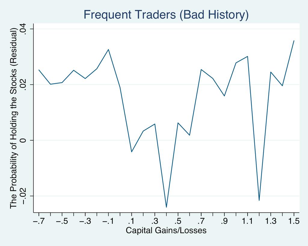
49 Appendix D: The Residual of the Probability of Holding the Stocks. 49

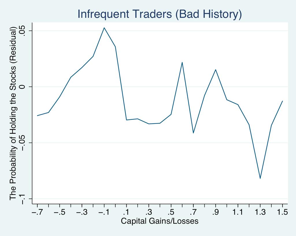
50 50