Normal Distribution. Definition A continuous rv X is said to have a normal distribution with. the pdf of X is

Transcription

1 Normal Distribution

2 Normal Distribution Definition A continuous rv X is said to have a normal distribution with parameter µ and σ (µ and σ 2 ), where < µ < and σ > 0, if the pdf of X is f (x; µ, σ) = 1 2πσ e (x µ)2 /(2σ 2 ) We use the notation X N(µ, σ 2 ) to denote that X is rormally distributed with parameters µ and σ 2.

3 Normal Distribution Proposition For X N(µ, σ 2 ), we have E(X ) = µ and V (X ) = σ 2

4 Normal Distribution Definition The normal distribution with parameter values µ = 0 and σ = 1 is called the standard normal distribution. A random variable having a standard normal distribution is called a standard normal random variable and will be denoted by Z. The pdf of Z is f (z; 0, 1) = 1 2π e z2 /2 < z < The graph of f (z; 0, 1) is called the standard normal (or z) curve. The cdf of Z is P(Z z) = z f (y; 0, 1)dy, which we will denote by Φ(z).

5 Normal Distribution Proposition If X has a normal distribution with mean µ and stadard deviation σ, then Z = X µ σ has a standard normal distribution. Thus P(a X b) = P( a µ Z b µ σ σ ) = Φ( b µ σ ) Φ(a µ σ ) P(X a) = Φ( a µ µ ) P(X b) = 1 Φ(b σ σ )

6 Normal Distribution

7 Normal Distribution Proposition {(100p)th percentile for N(µ, σ 2 )} = µ + {(100p)th percentile for N(0, 1)} σ

8 Normal Distribution

9 Normal Distribution Proposition Let X be a binomial rv based on n trials with success probability p. Then if the binomial probability histogram is not too skewed, X has approximately a normal distribution with µ = np and σ = npq, where q = 1 p. In particular, for x = a posible value of X, ( ) area under the normal curve P(X x) = B(x; n, p) to the left of x+0.5 x+0.5 np = Φ( ) npq In practice, the approximation is adequate provided that both np 10 and nq 10, since there is then enough symmetry in the underlying binomial distribution.

10 Normal Distribution

11 Normal Distribution A graphical explanation for ( ) area under the normal curve P(X x) = B(x; n, p) to the left of x+0.5 x+0.5 np = Φ( ) npq

12 Normal Distribution A graphical explanation for ( ) area under the normal curve P(X x) = B(x; n, p) to the left of x+0.5 x+0.5 np = Φ( ) npq

13 Normal Distribution

14 Normal Distribution Example (Problem 54) Suppose that 10% of all steel shafts produced by a certain process are nonconforming but can be reworked (rather than having to be scrapped). Consider a random sample of 200 shafts, and let X denote the number among these that are nonconforming and can be reworked. What is the (approximate) probability that X is between 15 and 25 (inclusive)?

15 Normal Distribution Example (Problem 54) Suppose that 10% of all steel shafts produced by a certain process are nonconforming but can be reworked (rather than having to be scrapped). Consider a random sample of 200 shafts, and let X denote the number among these that are nonconforming and can be reworked. What is the (approximate) probability that X is between 15 and 25 (inclusive)? In this problem n = 200, p = 0.1 and q = 1 p = 0.9. Thus np = 20 > 10 and nq = 180 > 10

16 Normal Distribution Example (Problem 54) Suppose that 10% of all steel shafts produced by a certain process are nonconforming but can be reworked (rather than having to be scrapped). Consider a random sample of 200 shafts, and let X denote the number among these that are nonconforming and can be reworked. What is the (approximate) probability that X is between 15 and 25 (inclusive)? In this problem n = 200, p = 0.1 and q = 1 p = 0.9. Thus np = 20 > 10 and nq = 180 > 10 P(15 X 25) = Bin(25; 200, 0.1) Bin(14; 200, 0.1) Φ( ) Φ( ) = Φ(0.3056) Φ( ) = =

17 Exponential Distribution

18 Exponential Distribution Definition X is said to have an exponential distribution with parameter λ(λ > 0) if the pdf of X is { λe λx x 0 f (x; λ) = 0 otherwise

19 Exponential Distribution

20 Exponential Distribution Proposition If X EXP(λ), then And the cdf for X is E(X ) = 1 λ and V (X ) = 1 λ 2 F (x; λ) = { 1 e λx x 0 0 x < 0

21 Exponential Distribution

22 Exponential Distribution Memoryless Property for any positive t and t 0. P(X t) = P(X t + t 0 X t 0 )

23 Exponential Distribution Memoryless Property P(X t) = P(X t + t 0 X t 0 ) for any positive t and t 0. In words, the distribution of additional lifetime is exactly the same as the original distribution of lifetime, so at each point in time the component shows no effect of wear. In other words, the distribution of remaining lifetime is independent of current age.

24

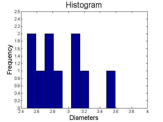
25 Example: There is a machine available for cutting corks intended for use in wine bottles. We want to find out the distribution of the diameters of the corks produced by that machine. Assume we have 10 samples produced by that machine and the diameters is recorded as following:

26

27

28

29

30

31

32 Sample Percentile

33 Sample Percentile Recall: The (100p)th percentile of the distribution of a continuous rv X, denoted by η(p), is defined by p = F (η(p)) = η(p) f (y)dy.

34 Sample Percentile Recall: The (100p)th percentile of the distribution of a continuous rv X, denoted by η(p), is defined by p = F (η(p)) = η(p) f (y)dy. In words, the (100p)th percentile η(p) is the X value such that there are 100p% X values below η(p).

35 Sample Percentile Recall: The (100p)th percentile of the distribution of a continuous rv X, denoted by η(p), is defined by p = F (η(p)) = η(p) f (y)dy. In words, the (100p)th percentile η(p) is the X value such that there are 100p% X values below η(p). Similarly, we can define sample percentile in the same manner, i.e. the (100p)th percentile x p is the value such that there are 100p% sample values below x p.

36 Sample Percentile Recall: The (100p)th percentile of the distribution of a continuous rv X, denoted by η(p), is defined by p = F (η(p)) = η(p) f (y)dy. In words, the (100p)th percentile η(p) is the X value such that there are 100p% X values below η(p). Similarly, we can define sample percentile in the same manner, i.e. the (100p)th percentile x p is the value such that there are 100p% sample values below x p. Unfortunately, x p may not be a sample value for some p.

37 Sample Percentile Recall: The (100p)th percentile of the distribution of a continuous rv X, denoted by η(p), is defined by p = F (η(p)) = η(p) f (y)dy. In words, the (100p)th percentile η(p) is the X value such that there are 100p% X values below η(p). Similarly, we can define sample percentile in the same manner, i.e. the (100p)th percentile x p is the value such that there are 100p% sample values below x p. Unfortunately, x p may not be a sample value for some p. e.g. for the previous example, what is the 35th percentile for the ten sample values?

38

39 Definition Assume we have a sample with size n. Order the n sample observations from smallest to largest. Then the ith smallest observation in the list is taken to be the [100(i 0.5)/n]th sample percentile.

40 Definition Assume we have a sample with size n. Order the n sample observations from smallest to largest. Then the ith smallest observation in the list is taken to be the [100(i 0.5)/n]th sample percentile. Remark: 1. Why i 0.5?

41 Definition Assume we have a sample with size n. Order the n sample observations from smallest to largest. Then the ith smallest observation in the list is taken to be the [100(i 0.5)/n]th sample percentile. Remark: 1. Why i 0.5? We regard the sample observation as being half in the lower group and half in the upper group.

42 Definition Assume we have a sample with size n. Order the n sample observations from smallest to largest. Then the ith smallest observation in the list is taken to be the [100(i 0.5)/n]th sample percentile. Remark: 1. Why i 0.5? We regard the sample observation as being half in the lower group and half in the upper group. e.g. if n = 9, then the sample median is the 5th largest observation and this observation is regarded as two parts: one in the lower half and one in the upper half.

43 Definition Assume we have a sample with size n. Order the n sample observations from smallest to largest. Then the ith smallest observation in the list is taken to be the [100(i 0.5)/n]th sample percentile. Remark: 1. Why i 0.5? We regard the sample observation as being half in the lower group and half in the upper group. e.g. if n = 9, then the sample median is the 5th largest observation and this observation is regarded as two parts: one in the lower half and one in the upper half. 2. Once the percentage values 100(i 0.5)/n(i = 1, 2,..., n) have been calculated, sample percentiles corresponding to intermediate percentages can be obtained by linear interpolation.

44

45 Example: for the previous example, the [100(i 0.5)/n]th sample percentile is tabulated as following: (1-.5)/10 = 5% 100(2-.5)/10 = 15% 100(3-.5)/10 = 25% (4-.5)/10 = 35% 100(5-.5)/10 = 45% (6-.5)/10 = 55% 100(7-.5)/10 = 65% 100(8-.5)/10 = 75% (9-.5)/10 = 85% 100(10-.5)/10 = 95%

46 Example: for the previous example, the [100(i 0.5)/n]th sample percentile is tabulated as following: (1-.5)/10 = 5% 100(2-.5)/10 = 15% 100(3-.5)/10 = 25% (4-.5)/10 = 35% 100(5-.5)/10 = 45% (6-.5)/10 = 55% 100(7-.5)/10 = 65% 100(8-.5)/10 = 75% (9-.5)/10 = 85% 100(10-.5)/10 = 95% The 10th percentile would be ( )/2 =

47

48 Idea for Quantile-Quantile Plot: 1. Determine the [100(i 0.5)/n]th sample percentile for a given sample.

49 Idea for Quantile-Quantile Plot: 1. Determine the [100(i 0.5)/n]th sample percentile for a given sample. 2. Find the corresponding [100(i 0.5)/n]th percentile from the population with the assumed distribution; for example, if the assumed distribution is standard normal, then find corresponding [100(i 0.5)/n]th percentile from the standard normal distribution.

50 Idea for Quantile-Quantile Plot: 1. Determine the [100(i 0.5)/n]th sample percentile for a given sample. 2. Find the corresponding [100(i 0.5)/n]th percentile from the population with the assumed distribution; for example, if the assumed distribution is standard normal, then find corresponding [100(i 0.5)/n]th percentile from the standard normal distribution. 3. Consider the (population percentile, sample percentile) pairs, i.e. ([100(i ) 0.5)/n]th percentile, ith smallest sample of the distribution observation

51 Idea for Quantile-Quantile Plot: 1. Determine the [100(i 0.5)/n]th sample percentile for a given sample. 2. Find the corresponding [100(i 0.5)/n]th percentile from the population with the assumed distribution; for example, if the assumed distribution is standard normal, then find corresponding [100(i 0.5)/n]th percentile from the standard normal distribution. 3. Consider the (population percentile, sample percentile) pairs, i.e. ([100(i ) 0.5)/n]th percentile, ith smallest sample of the distribution observation 4. Each pair plotted as a point on a two-dimensional coordinate system should fall close to a 45 line.

52 4. Each pair plotted as a point on a two-dimensional coordinate system should fall close to a 45 line. Substantial deviations of the plotted points from a 45 line cast doubt on the assumption that the distribution under consideration is the correct one. Probability Plot Idea for Quantile-Quantile Plot: 1. Determine the [100(i 0.5)/n]th sample percentile for a given sample. 2. Find the corresponding [100(i 0.5)/n]th percentile from the population with the assumed distribution; for example, if the assumed distribution is standard normal, then find corresponding [100(i 0.5)/n]th percentile from the standard normal distribution. 3. Consider the (population percentile, sample percentile) pairs, i.e. ([100(i ) 0.5)/n]th percentile, ith smallest sample of the distribution observation

53

54 Example 4.29: The value of a certain physical constant is known to an experimenter. The experimenter makes n = 10 independent measurements of this value using a particular measurement device and records the resulting measurement errors (error = observed value - true value). These observations appear in the following table. Percentage Sample Observation Percentage Sample Observation

55 Example 4.29: The value of a certain physical constant is known to an experimenter. The experimenter makes n = 10 independent measurements of this value using a particular measurement device and records the resulting measurement errors (error = observed value - true value). These observations appear in the following table. Percentage Sample Observation Percentage Sample Observation Is it plausible that the random variable measurement error has standard normal distribution?

56

57 We first find the corresponding population distribution percentiles, in this case, the z percentiles: Percentage Sample Observation z percentile Percentage Sample Observation z percentile

58

59

60

61 What about the first example? We are only interested in whether the ten sample observations come from a normal distribution.

62 What about the first example? We are only interested in whether the ten sample observations come from a normal distribution. Recall: {(100p)th percentile for N(µ, σ 2 )} = µ + {(100p)th percentile for N(0, 1)} σ

63 What about the first example? We are only interested in whether the ten sample observations come from a normal distribution. Recall: {(100p)th percentile for N(µ, σ 2 )} = µ + {(100p)th percentile for N(0, 1)} σ If µ = 0, then the pairs (σ [z percentile], observation) fall on a 45 line, which has slope 1.

64 What about the first example? We are only interested in whether the ten sample observations come from a normal distribution. Recall: {(100p)th percentile for N(µ, σ 2 )} = µ + {(100p)th percentile for N(0, 1)} σ If µ = 0, then the pairs (σ [z percentile], observation) fall on a 45 line, which has slope 1. Therefore the pairs ([z percentile], observation) fall on a line passing through (0,0) (i.e., one with y-intercept 0) but having slope σ rather than 1.

65 What about the first example? We are only interested in whether the ten sample observations come from a normal distribution. Recall: {(100p)th percentile for N(µ, σ 2 )} = µ + {(100p)th percentile for N(0, 1)} σ If µ = 0, then the pairs (σ [z percentile], observation) fall on a 45 line, which has slope 1. Therefore the pairs ([z percentile], observation) fall on a line passing through (0,0) (i.e., one with y-intercept 0) but having slope σ rather than 1. Now for µ 0, the y-intercept is µ instead of 0.

66

67 Normal Probability Plot A plot of the n pairs ([100(i 0.5)/n]th z percentile, ith smallest observation) on a two-dimensional coordinate system is called a normal probability plot. If the sample observations are in fact drawn from a normal distribution with mean value µ and standard deviation σ, the points should fall close to a straight line with slope σ and y-intercept µ. Thus a plot for which the points fall close to some straight line suggests that the assumption of a normal population distribution is plausible.

68

69 Percentage Sample Observation z percentile Percentage Sample Observation z percentile

70

71 A nonnormal population distribution can often be placed in one of the following three categories: 1. It is symmetric and has lighter tails than does a normal distribution; that is, the density curve declines more rapidly out in the tails than does a normal curve. 2. It is symmetric and heavy-tailed compared to a normal distribution. 3. It is skewed.

72

73 Symmetric and light-tailed : e.g. Uniform distribution

74

75 Symmetric and heavy-tailed: e.g. Cauchy distribution with pdf f (x) = 1/[π(1 + x 2 )] for < x <

76

77 Skewed: e.g. lognormal distribution

78

79 Some guidances for probability plot for normal distributions (from the book Fitting Equations to Data (2nd ed.) Daniel, Cuthbert, and Fed Wood, Wiley, New York, 1980)

80 Some guidances for probability plot for normal distributions (from the book Fitting Equations to Data (2nd ed.) Daniel, Cuthbert, and Fed Wood, Wiley, New York, 1980) 1. For sample size smaller than 30, there is typically greater variation in the apperance of the probability plot.

81 Some guidances for probability plot for normal distributions (from the book Fitting Equations to Data (2nd ed.) Daniel, Cuthbert, and Fed Wood, Wiley, New York, 1980) 1. For sample size smaller than 30, there is typically greater variation in the apperance of the probability plot. 2. Only for much larger sample sizes does a linear pattern generally predominate.

82 Some guidances for probability plot for normal distributions (from the book Fitting Equations to Data (2nd ed.) Daniel, Cuthbert, and Fed Wood, Wiley, New York, 1980) 1. For sample size smaller than 30, there is typically greater variation in the apperance of the probability plot. 2. Only for much larger sample sizes does a linear pattern generally predominate. Therefore, when a plot is based on a small sample size, only a very substantial departure from linearity should be taken as conclusive evidence of nonnorality.

83

84 Definition Consider a family of probability distributions involving two parameters, θ 1 and θ 2, and let F (x; θ 1, θ 2 ) denote the corresponding cdf s. The parameters θ 1 and θ 2 are said to be location and scale parameters, respectively, if F (x; θ 1, θ 2 ) is a function of (x θ 1 )/θ 2.

85 Definition Consider a family of probability distributions involving two parameters, θ 1 and θ 2, and let F (x; θ 1, θ 2 ) denote the corresponding cdf s. The parameters θ 1 and θ 2 are said to be location and scale parameters, respectively, if F (x; θ 1, θ 2 ) is a function of (x θ 1 )/θ 2. e.g. 1. Normal distributions N(µ, σ): F (x; µ, σ) = Φ( x µ σ ).

86 Definition Consider a family of probability distributions involving two parameters, θ 1 and θ 2, and let F (x; θ 1, θ 2 ) denote the corresponding cdf s. The parameters θ 1 and θ 2 are said to be location and scale parameters, respectively, if F (x; θ 1, θ 2 ) is a function of (x θ 1 )/θ 2. e.g. 1. Normal distributions N(µ, σ): F (x; µ, σ) = Φ( x µ σ ). 2. The extreme value distribution with cdf F (x; θ 1, θ 2 ) = 1 e e(x θ 1 )/θ 2

87

88 For Weibull distribution: F (x; α, β) = 1 e (x/β)α, the parameter β is a scale parameter but α is NOT a location parameter. α is usually referred to as a shape parameter.

89 For Weibull distribution: F (x; α, β) = 1 e (x/β)α, the parameter β is a scale parameter but α is NOT a location parameter. α is usually referred to as a shape parameter. Fortunately, if X has a Weibull distribution with shape parameter α and scale parameter β, then the transformed variable ln(x ) has an extreme value distribution with location parameter θ 1 = ln(β) and scale parameter θ 2 = 1/α.

90

91 The gamma distribution also has a shape parameter α. However, there is no transformation h( ) such that h(x ) has a distribution that depends only on location and scale parameters.

92 The gamma distribution also has a shape parameter α. However, there is no transformation h( ) such that h(x ) has a distribution that depends only on location and scale parameters. Thus, before we construct a probability plot, we have to estimate the shape parameter from the sample data.

93 Jointly Distributed Random Variables

94 Jointly Distributed Random Variables Consider tossing a fair die twice. Then the outcomes would be (1,1) (1,2) (1,3) (1,4) (1,5) (1,6) (2,1) (2,2) (2,3) (2,4) (2,5) (2,6) (6,1) (6,2) (6,3) (6,4) (6,5) (6,6) and the probability for each outcome is 1 36.

95 Jointly Distributed Random Variables Consider tossing a fair die twice. Then the outcomes would be (1,1) (1,2) (1,3) (1,4) (1,5) (1,6) (2,1) (2,2) (2,3) (2,4) (2,5) (2,6) (6,1) (6,2) (6,3) (6,4) (6,5) (6,6) and the probability for each outcome is If we define two random variables by X = the outcome of the first toss and Y = the outcome of the second toss,

96 Jointly Distributed Random Variables Consider tossing a fair die twice. Then the outcomes would be (1,1) (1,2) (1,3) (1,4) (1,5) (1,6) (2,1) (2,2) (2,3) (2,4) (2,5) (2,6) (6,1) (6,2) (6,3) (6,4) (6,5) (6,6) and the probability for each outcome is If we define two random variables by X = the outcome of the first toss and Y = the outcome of the second toss, then the outcome for this experiment (two tosses) can be describe by the random pair (X, Y ),

97 Jointly Distributed Random Variables Consider tossing a fair die twice. Then the outcomes would be (1,1) (1,2) (1,3) (1,4) (1,5) (1,6) (2,1) (2,2) (2,3) (2,4) (2,5) (2,6) (6,1) (6,2) (6,3) (6,4) (6,5) (6,6) and the probability for each outcome is If we define two random variables by X = the outcome of the first toss and Y = the outcome of the second toss, then the outcome for this experiment (two tosses) can be describe by the random pair (X, Y ), and the probability for any possible value of that random pair (x, y) is 1 36.

98 Jointly Distributed Random Variables

99 Jointly Distributed Random Variables Definition Let X and Y be two discrete random variables defined on the sample space S of an experiment. The joint probability mass function p(x, y) is defined for each pair of numbers (x, y) by p(x, y) = P(X = x and Y = y) (It must be the case that p(x, y) 0 and x y p(x, y) = 1.) For any event A consisting of pairs of (x, y), the probability P[(X, Y ) A] is obtained by summing the joint pmf over pairs in A: P[(X, Y ) A] = p(x, y) (x,y) A

100 Jointly Distributed Random Variables

101 Jointly Distributed Random Variables Example (Problem 75) A restaurant serves three fixed-price dinners costing $12, $15, and $20. For a randomly selected couple dinning at this restaurant, let X = the cost of the man s dinner and Y = the cost of the woman s dinner. If the joint pmf of X and Y is assumed to be y p(x, y) x

102 Jointly Distributed Random Variables Example (Problem 75) A restaurant serves three fixed-price dinners costing $12, $15, and $20. For a randomly selected couple dinning at this restaurant, let X = the cost of the man s dinner and Y = the cost of the woman s dinner. If the joint pmf of X and Y is assumed to be y p(x, y) x a. What is the probability for them to both have the $12 dinner?

103 Jointly Distributed Random Variables Example (Problem 75) A restaurant serves three fixed-price dinners costing $12, $15, and $20. For a randomly selected couple dinning at this restaurant, let X = the cost of the man s dinner and Y = the cost of the woman s dinner. If the joint pmf of X and Y is assumed to be y p(x, y) x a. What is the probability for them to both have the $12 dinner? b. What is the probability that they have the same price dinner?

104 Jointly Distributed Random Variables Example (Problem 75) A restaurant serves three fixed-price dinners costing $12, $15, and $20. For a randomly selected couple dinning at this restaurant, let X = the cost of the man s dinner and Y = the cost of the woman s dinner. If the joint pmf of X and Y is assumed to be y p(x, y) x a. What is the probability for them to both have the $12 dinner? b. What is the probability that they have the same price dinner? c. What is the probability that the man s dinner cost $12?

105 Jointly Distributed Random Variables

106 Jointly Distributed Random Variables Definition Let X and Y be two discrete random variables defined on the sample space S of an experiment with joint probability mass function p(x, y). Then the pmf s of each one of the variables alone are called the marginal probability mass functions, denoted by p X (x) and p Y (y), respectively. Furthermore, p X (x) = y p(x, y) and p Y (y) = x p(x, y)

107 Jointly Distributed Random Variables

108 Jointly Distributed Random Variables Example (Problem 75) continued: The marginal probability mass functions for the previous example is calculated as following: y p(x, y) p(x, ) x p(, y)

109 Jointly Distributed Random Variables

110 Jointly Distributed Random Variables Definition Let X and Y be continuous random variables. A joint probability density function f (x, y) for these two variables is a function satisfying f (x, y) 0 and f (x, y)dxdy = 1. For any two-dimensional set A P[(X, Y ) A] = f (x, y)dxdy In particular, if A is the two-dimensilnal rectangle {(x, y) : a x b, c y d}, then P[(X, Y ) A] = P(a X b, c Y d) = A b d a c f (x, y)dydx

111 Jointly Distributed Random Variables

112 Jointly Distributed Random Variables Definition Let X and Y be continuous random variables with joint pdf f (x, y). Then the marginal probability density functions of X and Y, denoted by f X (x) and f Y (y), respectively, are given by f X (x) = f Y (y) = f (x, y)dy f (x, y)dx for < x < for < y <

113 Jointly Distributed Random Variables

114 Jointly Distributed Random Variables Example (variant of Problem 12) Two components of a minicomputer have the following joint pdf for their useful lifetimes X and Y : { xe (x+y) x 0 and y 0 f (x, y) = 0 otherwise

115 Jointly Distributed Random Variables Example (variant of Problem 12) Two components of a minicomputer have the following joint pdf for their useful lifetimes X and Y : { xe (x+y) x 0 and y 0 f (x, y) = 0 otherwise a. What is the probability that the lifetimes of both components excceed 3?

116 Jointly Distributed Random Variables Example (variant of Problem 12) Two components of a minicomputer have the following joint pdf for their useful lifetimes X and Y : { xe (x+y) x 0 and y 0 f (x, y) = 0 otherwise a. What is the probability that the lifetimes of both components excceed 3? b. What are the marginal pdf s of X and Y?

117 Jointly Distributed Random Variables Example (variant of Problem 12) Two components of a minicomputer have the following joint pdf for their useful lifetimes X and Y : { xe (x+y) x 0 and y 0 f (x, y) = 0 otherwise a. What is the probability that the lifetimes of both components excceed 3? b. What are the marginal pdf s of X and Y? c. What is the probability that the lifetime X of the first component excceeds 3?

118 Jointly Distributed Random Variables Example (variant of Problem 12) Two components of a minicomputer have the following joint pdf for their useful lifetimes X and Y : { xe (x+y) x 0 and y 0 f (x, y) = 0 otherwise a. What is the probability that the lifetimes of both components excceed 3? b. What are the marginal pdf s of X and Y? c. What is the probability that the lifetime X of the first component excceeds 3? d. What is the probability that the lifetime of at least one component excceeds 3?