Duration Models: Parametric Models

Transcription

1 Duration Models: Parametric Models Brad 1 1 Department of Political Science University of California, Davis January 28, 2011

2

3 Parametric Models Some Motivation for Parametrics Consider the hazard rate: dh(t) dt > 0, Hazard increasing wrt time. dh(t) dt < 0, Hazard decreasing wrt time. dh(t) dt = 0, Hazard flat wrt time.

4 Parametric Models Parametric models give structure (shape) to the hazard function. N.B.: the structure is a function of the c.d.f., not necessarily of the real world.... though some c.d.f.s do a good job of approximating some failure-time processes. Any c.d.f. with positive support on the real number line will work. Lots of choices: exponential, Weibull, gamma, Gompertz, log-normal, log-logistic... etc.

5

6 Parametric Models For parametrics, we work with standard likelihood methods. Specify a distribution function and write out the log-likelihood for the data. The question is, which distribution function? In all software programs/computing environments, youre given a menu. Stata:streg, R:survreg, eha

7 Parametric Models Advantages of parametric models? If S(t) is known to follow, or closely approximate a known distribution, then estimates will be consistent the the theoretical survivor function. Unlike K-M or Cox (discussed later), the hazard may be used for forecasting (under KM or Cox, the hazard is only defined up until the last observed failure). Will return smooth functions of h(t) or S(t).

8 Parametric Models As noted, there are a wide variety of choices. I sometimes refer to these choices as plug and play estimators. Why? Consider the survivor function: S(t) = Pr(T > t) = t t f (u)d(u) = 1 f (u)d(u) = 1 F (t) 0 (1) If we know this function follows some distribution, then we write a likelihood function in terms of this distribution... If it follows a different distribution, just replace the previous likelihood with another pdf.

9 Parametric Models Most texts, including ours, typically begin with the exponential distribution. The reason is easy: it s an easy distribution to work with and visualize. It also may be unrealistic in many settings. The basic feature: the hazard rate is flat wrt time. That is: h(t) = λ (2)

10 Parametric Models Recall from the first week: where Substituting λ into (3), S(t) = exp{ H(t)} (3) H(t) = t 0 h(u)du t S(t) = exp{ λdu} 0 and so S(t) = exp( λt) This is the survivor function for the exponential distribution.

11 Parametric Models Since we know f (t) = h(t)s(t) then f (t) = λ exp( λt) This is the pdf of a random variable T that is exponentially distributed. Note how the unconditional probability of failure, f (t), handles censored cases. Consider the hazard function:

12

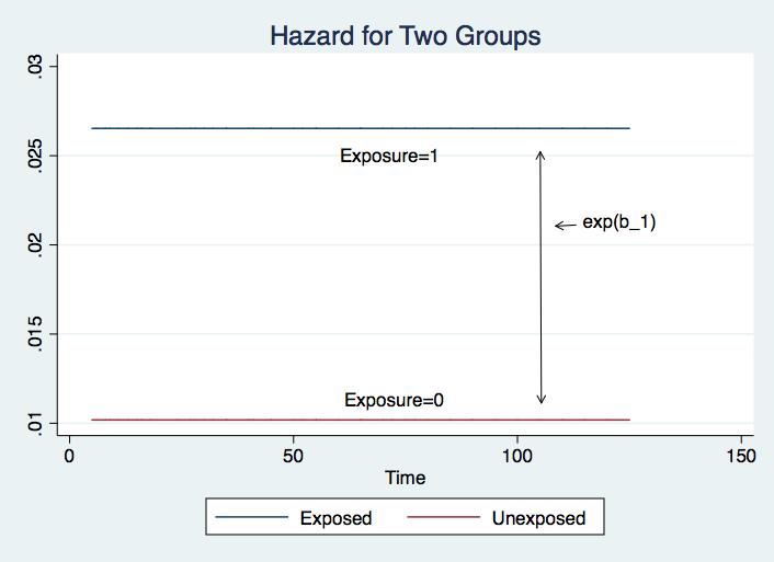
13 Parametric Models What is λ? Or put differently, where are the predictor variables? Typically λ will be parameterized in terms of regression coefficients and covariates, X. A model: h(t) = λ = exp(β 0 + β 1 T ) Suppose T is a treatment indicator and we re interested in the hazard of failure for the treated and untreated.

14 Parametric Models Two hazards: h(t T =1 ) = exp(β 0 + β 1 ) h(t T =0 ) = exp(β 0 ) If we plotted the hazards, we would have two parallel lines separated by exp(β 1 ). Or analogously, if we want to compare hazards: h(t T =1 ) h(t T =0 ) = exp(β 0 + β 1 ) exp(β 0 ) item 4- This expression must simplify to exp(β 1 ).

15 Parametric Models In words (sort of)...the ratio of the treated to the untreated simplifies to exp(β 1 ). So all we need to know to know the differences in the hazards is the coefficient for the treated. This is an important result because it shows the hazards are proportional hazards. Some simulated data. h(t) = (Z) Let Z denote whether or not a subject was exposed to some condition.

16 Parametric Models Since β 1 is positive, this implies exposure increases the risk. The hazard is higher for the exposed than for the unexposed. Treatment estimate is.96 implies difference in hazard is exp(.96) 2.6 Risk for exposed is about 2.6 times greater than for the unexposed. Consider the hazards:

17

18 Parametric Models PH property is important to understand. By way of analogy, think about what odds ratios are in a logit-type setting or recall the ordered logit model: the OR are invariant to the scale scores. The proportional difference in hazards is invariant to time. So under the exponential we are making two assumptions: 1. The hazards are flat wrt time. 2. The difference in hazards across levels of a covariate is a fixed proportion. Which is the stronger assumption?

19 Parametric Models Note that even with the PH assumption, we are not saying (in general) the hazards are invariant to time (though in the exponential case, we are). The hazards may change but the proportional difference between (say) two groups, does not change. That s the basic result of proportionality. Suppose it does not hold. Then what? Consider another model that relaxes the assumption of flat hazards (but not the PH assumption).

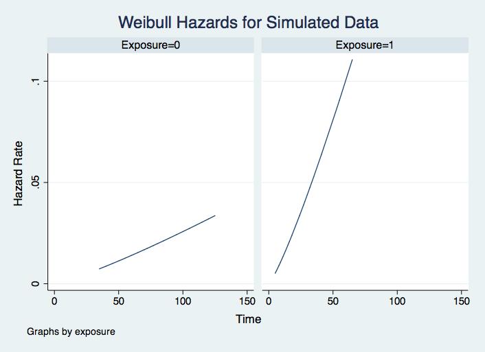
20 Parametric Models: Weibull A more flexible distribution function is given by the Weibull. Named for Waloddi Weibull, who derived it (1939, 1951) Why more general than the exponential? It is a two-parameter distribution: h(t) = λpt p 1 (4) where λ is a positive scale parameter and p is a shape parameter. Note: p > 1, the hazard rate is monotonically increasing with time. p < 1, the hazard rate is monotonically decreasing with time. p = 1, the hazard is flat.

21 Parametric Models: Weibull Thus if p = 1 then h(t) = λ1t 1 1 = λ. (5) Thus demonstrating that the exponential model is nested within the Weibull. For this reason (and for many other reasons), the Weibull is the most commonly applied parametric model in survival analysis. As with the exponential, the scale parameter λ is usually expressed in terms of covariates, exp(β k x i ). Hazard functions plotted for different p:

22

23 Parametric Models: Weibull Using the connection between S(t) and the cumulative hazard (see eq. [3]), the Weibull survivor function is given by t S(t) = exp{ λpu p 1 du} = exp( λt p ). 0 And since the pdf is h(t)s(t), the density for a random variable T distributed as a Weibull is f (t) = λpt p 1 exp( λt p ). Suppose we estimate a Weibull hazard using the data from before.

24

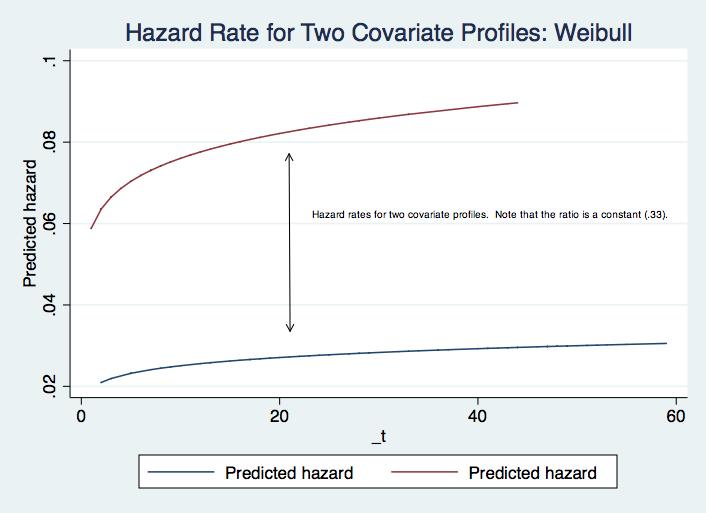
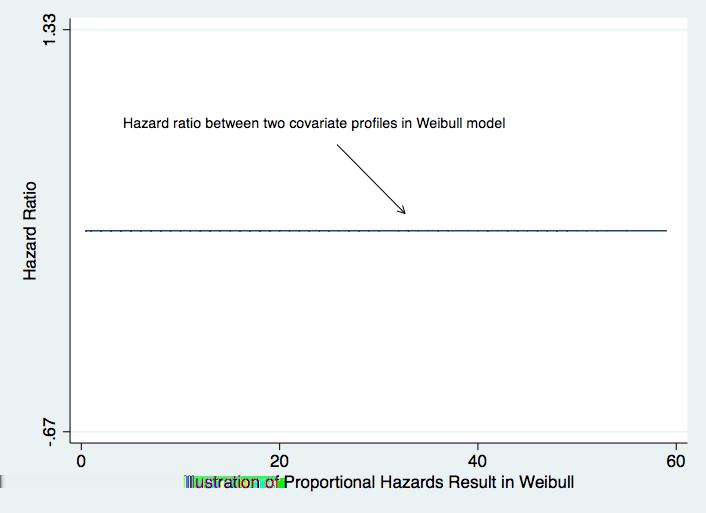
25 Parametric Models: Weibull Note: h(t E ) h(t NE ) = exp(β 0 + β 1 )pt p 1 exp(β 0 )pt p 1 = exp(β 1 ) In other words, the Weibull model is a proportional hazards model. So unlike the exponential, the hazards can change wrt time but like the exponential, the ratio of the hazards is a constant. They are offset by a proportionality factor of exp(β).

26 Parametric Models: Weibull The Weibull (and therefore) the exponential are interesting models. They are both proportional hazards models as well as accelerated failure time models. In other words, one can estimate the model in terms of the hazards or in terms of the survival times and reproduce equivalent results from different parameterizations. Under the PH model, the covariates are a multiplicative effect with respect to the baseline hazard function (see previous slide). Under the AFT, the covariates are multiplicative wrt the survival time.

27 Parametric Models: Weibull Proportional Hazards: h(t x) = h 0 t exp(β1x 1 + β 2 x β j x j ) Accelerated Failure Time: log(t ) = β 0 + β 1 x 1 + β 2 x β j x j + σɛ where ɛ is a stochastic disturbance term with type-1 extreme-value distribution scaled by σ. Note: σ = 1/p. Extreme-value has a close connection to Weibull: the distribution of the log of a Weibull distributed random variable yields a type-1 extreme value distribution.

28 Parametric Models: Weibull In the AFT formulation, the coefficients are sometimes referred to as acceleration factors. They give information about how the survival times are differentially accelerated for different levels of a covariate. Suppose we estimate a treatment effect for two groups: D and H. Imagine the estimated treatment effect yields a coefficient of 7. That is, group H is estimated to survive 7 times longer than group D. S D (t) = S H (7t) If D are dogs and H are humans, the acceleration factor suggests human lifespans are stretched out 7 times longer than dogs. (Example from K and K, p. 266.)

29 Parametric Models: Weibull Important to be aware of what your software is doing! The PH coefficients inform us about the hazard (i.e. risk). The AFT coefficients inform us about survival. Therefore, the coefficients will be signed differently.

30 Parametric Models: Weibull Weibull hazard is monotonic. Log-logistic and log-normal allow for nonmonotonic hazards. Both estimated only as AFT models: log(t ) = βx + σɛ. The AFT for each of these models has two parameters.

31 Parametric Models: Log-Logistic The log-logistic is one choice for non-monotonic hazards: h(t) = λptp λt p h(t) increases and then decreases if p > 1; monotonically decreasing when p 1.

32

33 Parametric Models: Log-Logistic Again, λ gives information on the covariates (i.e. here is where the regression coefficients are. While the log-logistic is not a PH model, it is a proportional odds model. Recall what this is from your previous course on MLE. Survivor function: S(t) = λt p = λtp 1 + λt p Substitute exp(β) in for λ and you can see the connection back to the logistic cdf.

34 Parametric Models: Log-Logistic The odds of failure: 1 S(t) S(t) = λt p 1+λt p 1 1+λt p = λt p In terms of parameters, exponentiating β will give the acceleration factor. Interpretation is really quite similar to a logit model (but it is not exactly the same!). Other models?

35 Parametric Models: Estimation Previous can be estimated through MLE Imagine n observations upon which t 1, t 2,... t n duration times are measured. Assume conditional independence of t i (may be herculean assumption; more later) Specify a PDF (or CDF); if f (t) is derived, S(t) easily follows Write out likelihood function and maximize (standard algorithm is Newton-Raphson)

36 Parametric Models: Estimation Generic Likelihood: L = n {f (t i )} δ i {S(t i )} 1 δ i i=1 where δ i is the censoring (failure) indicator. Example: Weibull Survivor function f (t) = λpt p 1 exp (λt p ) S(t) = exp (λt p ) The likelihood of the t duration times: n L = {λpt p 1 exp (λt p )} δ i {exp (λt p )} 1 δ i i=1

37 Getting Our Hands Dirty The only way to learn is to do. Useful to consider estimation and interpretation of some parametric models. Examples are based on cabinet duration data and most of the code is in Stata. Stata do file is accessible on SmartSite and website.

38 Exponential Cabinet duration as a function of post-election negotiations indicator and formation attempts. Table: Estimation results : PH Exponential Variable Coefficient (Std. Err.) format (0.039) postelec (0.124) Intercept (0.106)

39 Exponential Coefficients are in PH scale so a positively signed coefficient implies the hazard is increasing as a function of x. Post-election negotiations lowers the hazard; increased number of formation attempts increase the hazard. Graphical display of two covariate profiles.

40

41 Exponential Turn attention to the Stata examples (we will do this in class). Consider the AFT model. Recall the AFT model: log(t ) = β k x i + σɛ If ɛ is type-1 extreme value (aka Gumbel) then the Weibull is obtained. If σ = p = 1 then the exponential is obtained. The coefficients are multiples of the survivor function.

42 Exponential Table: Estimation results : AFT Exponential Variable Coefficient (Std. Err.) format (0.039) postelec (0.124) Intercept (0.106)

43 Exponential Contrast the PH and AFT models. Under the exponential, the signs shift but the coefficients are unchanged in value. Sign shift makes sense: AFT formulation tells us about survivorship. AFT Hazard: h o (t) exp (xβ) = exp (β 0 + xβ k ) Solving for t: t = [ log(s(t)] exp(β 0 + β 1 postelec) If t =.5, we solve for the median survival time. Turn back to the Stata examples.

44 Exponential From the application, note the equivalency of the two models. Note also that the ratio of two survival times for two covariate profiles (i.e. X = 1 vs. X = 0) will be constant and proportional wrt S(t). Hence either parameterization exhibits proportionality. Weibull example.

45 Weibull Under the exponential the hazard is flat.. Under the Weibull: h(t) = λpt p 1 (6) λ is positive scale parameter; p is the shape parameter. p > 1, the hazard rate is monotonically increasing with time. p < 1, the hazard rate is monotonically decreasing with time. p = 1, the hazard is flat, i.e. exponential. Note that λ corresponds to covariates: exp(β k x i )

46 Weibull hazards Consider application again. Table: Estimation results : PH Weibull Variable Coefficient (Std. Err.) Equation 1 : t format (0.039) postelec (0.129) Intercept (0.199) Equation 2 : ln p Intercept (0.050)

47 Weibull Coefficients are interpreted as before though now we have an additional parameter. p > 1 implying rising hazards for this model. Consider the hazard rates for two covariate profiles.

48

49 Weibull Observations? Note the shape is governed by p... But the difference in the two hazards are proportional. Looks may be deceiving; perhaps you think the lines show nonproportionality. Back to the application.

50

51 Weibull Consider the AFT formulation Table: Estimation results : weibull Variable Coefficient (Std. Err.) Equation 1 : t format (0.035) postelec (0.113) Intercept (0.096) Equation 2 : ln p Intercept (0.050)

52 Weibull Similar interpretation is afforded this model as was the case with the exponential AFT. Note under the AFT: S(t) = exp( λt p ) Therefore, t = [ log S(t)] 1/p 1. λ 1/p Expressing 1 in terms of the model parameters, we obtain λ 1/p t = [ log S(t)] 1/p exp(β 0 + β k x) As with the exponential, let q denote some S(t), then we can estimate S(t) for some value q: t = [ log S(q)] 1/p exp(β 0 + β k x) So for the median, q =.5. Go to example.

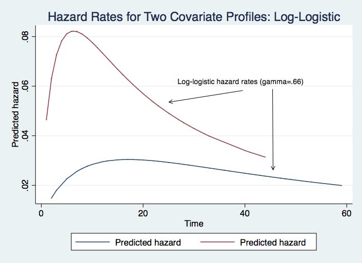
53 Log-Logistic Consider now the log-logistic. The log-logistic is only an AFT model. Table: Estimation results : AFT: Log-Logistic Variable Coefficient (Std. Err.) Equation 1 : t format (0.050) postelec (0.130) Intercept (0.126) Equation 2 : ln gam Intercept (0.051)

54

55 Log-Logistic Consider now the log-logistic. The log-logistic is only an AFT model. Note that Stata reports γ as the shape parameter. This is the inverse of p. Consider the survivor function: S(t) = 1 1+λt p = 1 1+(λ 1/p t)p Suppose we solve for t: t = [ 1 S(t) 1]1/p 1 λ 1/p Express the second term in terms of covariates, we obtain: t = [ 1 S(t) 1]1/p exp(β 0 + β k x) To the example.

56 Log-Logistic Because the log-logistic is AFT and proportional odds, this ratio should be equivalent to the acceleration factor (i.e. the odds ratio exp(β 1 )). So this too is a proportional model... in the odds ratios. This assumption may not hold.

57 Many Applications These are plug and play estimators. They are easy to do. Let s run through some illustrations, first in Stata and then in R I use the cabinet duration data.

58 Weibull. streg invest polar numst format postelec caretakr, dist(weib) time nolog failure _d: analysis time _t: censor durat Weibull regression -- accelerated failure-time form No. of subjects = 314 Number of obs = 314 No. of failures = 271 Time at risk = LR chi2(6) = Log likelihood = Prob > chi2 = _t Coef. Std. Err. z P> z [95% Conf. Interval] invest polar numst format postelec caretakr _cons /ln_p p /p

59 Exponential. streg invest polar numst format postelec caretakr, dist(exp) time nolog failure _d: analysis time _t: censor durat Exponential regression -- accelerated failure-time form No. of subjects = 314 Number of obs = 314 No. of failures = 271 Time at risk = LR chi2(6) = Log likelihood = Prob > chi2 = _t Coef. Std. Err. z P> z [95% Conf. Interval] invest polar numst format postelec caretakr _cons

60 Log-logistic. streg invest polar numst format postelec caretakr, dist(loglog) time nolog failure _d: analysis time _t: censor durat Log-logistic regression -- accelerated failure-time form No. of subjects = 314 Number of obs = 314 No. of failures = 271 Time at risk = LR chi2(6) = Log likelihood = Prob > chi2 = _t Coef. Std. Err. z P> z [95% Conf. Interval] invest polar numst format postelec caretakr _cons /ln_gam gamma

61 Log-normal. streg invest polar numst format postelec caretakr, dist(lognorm) time nolog failure _d: analysis time _t: censor durat Log-normal regression -- accelerated failure-time form No. of subjects = 314 Number of obs = 314 No. of failures = 271 Time at risk = LR chi2(6) = Log likelihood = Prob > chi2 = _t Coef. Std. Err. z P> z [95% Conf. Interval] invest polar numst format postelec caretakr _cons /ln_sig sigma

62 Weibull > cab.weib<-survreg(surv(durat,censor)~invest + polar + numst + + format + postelec + caretakr,data=cabinet, + dist= weibull ) > > summary(cab.weib) Call: survreg(formula = Surv(durat, censor) ~ invest + polar + numst + format + postelec + caretakr, data = cabinet, dist = "weibull") Value Std. Error z p (Intercept) e-120 invest e-03 polar e-05 numst e-06 format e-03 postelec e-11 caretakr e-11 Log(scale) e-07 Scale= Weibull distribution Loglik(model)= Loglik(intercept only)= Chisq= on 6 degrees of freedom, p= 0 Number of Newton-Raphson Iterations: 5 n= 314

63 Log-Logistic > cab.ll<-survreg(surv(durat,censor)~invest + polar + numst + + format + postelec + caretakr,data=cabinet, + dist= loglogistic ) > > summary(cab.ll) Call: survreg(formula = Surv(durat, censor) ~ invest + polar + numst + format + postelec + caretakr, data = cabinet, dist = "loglogistic") Value Std. Error z p (Intercept) e-65 invest e-03 polar e-05 numst e-05 format e-03 postelec e-07 caretakr e-08 Log(scale) e-28 Scale= Log logistic distribution Loglik(model)= Loglik(intercept only)= Chisq= on 6 degrees of freedom, p= 0 Number of Newton-Raphson Iterations: 4 n= 314

64 > ##Log-Normal can be fit using survreg: > > cab.ln<-survreg(surv(durat,censor)~invest + polar + numst + + format + postelec + caretakr,data=cabinet, + dist= lognormal ) > > summary(cab.ln) Call: survreg(formula = Surv(durat, censor) ~ invest + polar + numst + format + postelec + caretakr, data = cabinet, dist = "lognormal") Value Std. Error z p (Intercept) e-57 invest e-03 polar e-05 numst e-06 format e-03 postelec e-07 caretakr e-05 Log(scale) e-01 Scale= 1.01 Log Normal distribution Loglik(model)= Loglik(intercept only)= Chisq= on 6 degrees of freedom, p= 0 Number of Newton-Raphson Iterations: 4 n= 314

65 Comparing Log-Likelihoods (note: non-nested models). I did this in R: anova(cab.weib, cab.ln, cab.ll) 1 invest + polar + numst + format + postelec + caretakr 2 invest + polar + numst + format + postelec + caretakr 3 invest + polar + numst + format + postelec + caretakr Resid. Df -2*LL Test Df Deviance P(> Chi ) NA NA NA = NA = NA

66 Back to Stata: Generalized Gamma. streg invest polar numst format postelec caretakr, dist(gamma) nolog failure _d: analysis time _t: censor durat Gamma regression -- accelerated failure-time form No. of subjects = 314 Number of obs = 314 No. of failures = 271 Time at risk = LR chi2(6) = Log likelihood = Prob > chi2 = _t Coef. Std. Err. z P> z [95% Conf. Interval] invest polar numst format postelec caretakr _cons /ln_sig /kappa sigma

67 Adjudication Lots of Choices Selection can be arbitrary If parametrically nested, standard LR tests apply. Encompassing Distribution: generalized gamma: f (t) = λp(λt)pκ 1 exp[ (λt) p ] Γ(κ) When κ = 1, the Weibull is implied; when κ = p = 1, the exponential distribution is implied; when κ = 0, the log-normal distribution is implied; and when p = 1, the gamma distribution is implied. In illustrations above, verify that Weibull would be preferred model among the choices. AIC ( 2(log L) + 2(c + p + 1)) also confirms Weibull is preferred model among choices. (7)

68 Survivor Functions Cabinet Duration Figure: The figure graphs the generalized gamma and Weibull survivor functions for the cabinet duration data. The Weibull estimates are denoted by the O symbol and the generalized gamma estimates are

69 denoted by the line.

70 Table: AIC and Log-Likelihoods for Cabinet Models Model Log-Likelihood AIC Exponential Weibull Log-Logistic Log-Normal Gompertz Generalized Gamma