Optimization Models for Quantitative Asset Management 1

Transcription

1 Optimization Models for Quantitative Asset Management 1 Reha H. Tütüncü Goldman Sachs Asset Management Quantitative Equity Joint work with D. Jeria, GS Fields Industrial Optimization Seminar November 13, This material is provided for educational purposes only and should not be construed as investment advice or an offer or solicitation to buy or sell securities.

2 Outline 1 Multi-Portfolio Optimization 2 Dynamic Portfolio Management

3 Quantitative Portfolio Management A quantitative portfolio manager seeks to find the optimal trade-off among three competing concerns: Maximize expected portfolio return Minimized portfolio risk (in absolute or relative terms) Minimize trading costs (t-costs, from now on) Trading costs can be a significant part of a large manager s utility. Different approaches to managing trading costs carefully will be the main focus of this talk.

4 Quantitative Portfolio Management A quantitative portfolio manager seeks to find the optimal trade-off among three competing concerns: Maximize expected portfolio return Minimized portfolio risk (in absolute or relative terms) Minimize trading costs (t-costs, from now on) Trading costs can be a significant part of a large manager s utility. Different approaches to managing trading costs carefully will be the main focus of this talk.

5 Quantitative Portfolio Management A quantitative portfolio manager seeks to find the optimal trade-off among three competing concerns: Maximize expected portfolio return Minimized portfolio risk (in absolute or relative terms) Minimize trading costs (t-costs, from now on) Trading costs can be a significant part of a large manager s utility. Different approaches to managing trading costs carefully will be the main focus of this talk.

6 Quantitative Portfolio Management A quantitative portfolio manager seeks to find the optimal trade-off among three competing concerns: Maximize expected portfolio return Minimized portfolio risk (in absolute or relative terms) Minimize trading costs (t-costs, from now on) Trading costs can be a significant part of a large manager s utility. Different approaches to managing trading costs carefully will be the main focus of this talk.

7 Quantitative Portfolio Management A quantitative portfolio manager seeks to find the optimal trade-off among three competing concerns: Maximize expected portfolio return Minimized portfolio risk (in absolute or relative terms) Minimize trading costs (t-costs, from now on) Trading costs can be a significant part of a large manager s utility. Different approaches to managing trading costs carefully will be the main focus of this talk.

8 Generic Portfolio Optimization Problem Usual framework: n securities, expected returns given by µ and covariance matrix Σ. A portfolio of the available securities is denoted by the vector x = (x 1, x 2,..., x n ). Let x 0 denote the initial portfolio and let t = x x 0 denote the trade vector. Representing portfolio constraints in the generic form x X, we can formulate a simple optimization problem: max µ T x λx T Σx φtc(t) T t s.t. x X. Above λ and φ represent the risk and t-cost aversion respectively and TC represents the unit t-cost function. This is one of the three alternative formulations of Markowitz mean-variance optimization (MVO) problem.

9 Generic Portfolio Optimization Problem Usual framework: n securities, expected returns given by µ and covariance matrix Σ. A portfolio of the available securities is denoted by the vector x = (x 1, x 2,..., x n ). Let x 0 denote the initial portfolio and let t = x x 0 denote the trade vector. Representing portfolio constraints in the generic form x X, we can formulate a simple optimization problem: max µ T x λx T Σx φtc(t) T t s.t. x X. Above λ and φ represent the risk and t-cost aversion respectively and TC represents the unit t-cost function. This is one of the three alternative formulations of Markowitz mean-variance optimization (MVO) problem.

10 Generic Portfolio Optimization Problem Usual framework: n securities, expected returns given by µ and covariance matrix Σ. A portfolio of the available securities is denoted by the vector x = (x 1, x 2,..., x n ). Let x 0 denote the initial portfolio and let t = x x 0 denote the trade vector. Representing portfolio constraints in the generic form x X, we can formulate a simple optimization problem: max µ T x λx T Σx φtc(t) T t s.t. x X. Above λ and φ represent the risk and t-cost aversion respectively and TC represents the unit t-cost function. This is one of the three alternative formulations of Markowitz mean-variance optimization (MVO) problem.

11 Typical portfolio constraints Compliance and client constraints e.g., a restricted trade list Exposure constraints e.g., limits on active bets on securities, industries, sectors, etc. Trade constraints e.g., limit trades to x% of the average daily volume (ADV) Cardinality constraints e.g., limits on the number of trades or holdings Threshold constraints e.g., do not hold a position smaller than x% of the portfolio Others e.g., limit distance to a model portfolio However, Constraints... accumulate like useless items in a closet until their cumulative effect is too large to ignore. (R. Grinold)

12 Typical portfolio constraints Compliance and client constraints e.g., a restricted trade list Exposure constraints e.g., limits on active bets on securities, industries, sectors, etc. Trade constraints e.g., limit trades to x% of the average daily volume (ADV) Cardinality constraints e.g., limits on the number of trades or holdings Threshold constraints e.g., do not hold a position smaller than x% of the portfolio Others e.g., limit distance to a model portfolio However, Constraints... accumulate like useless items in a closet until their cumulative effect is too large to ignore. (R. Grinold)

13 Typical portfolio constraints Compliance and client constraints e.g., a restricted trade list Exposure constraints e.g., limits on active bets on securities, industries, sectors, etc. Trade constraints e.g., limit trades to x% of the average daily volume (ADV) Cardinality constraints e.g., limits on the number of trades or holdings Threshold constraints e.g., do not hold a position smaller than x% of the portfolio Others e.g., limit distance to a model portfolio However, Constraints... accumulate like useless items in a closet until their cumulative effect is too large to ignore. (R. Grinold)

14 Typical portfolio constraints Compliance and client constraints e.g., a restricted trade list Exposure constraints e.g., limits on active bets on securities, industries, sectors, etc. Trade constraints e.g., limit trades to x% of the average daily volume (ADV) Cardinality constraints e.g., limits on the number of trades or holdings Threshold constraints e.g., do not hold a position smaller than x% of the portfolio Others e.g., limit distance to a model portfolio However, Constraints... accumulate like useless items in a closet until their cumulative effect is too large to ignore. (R. Grinold)

15 Typical portfolio constraints Compliance and client constraints e.g., a restricted trade list Exposure constraints e.g., limits on active bets on securities, industries, sectors, etc. Trade constraints e.g., limit trades to x% of the average daily volume (ADV) Cardinality constraints e.g., limits on the number of trades or holdings Threshold constraints e.g., do not hold a position smaller than x% of the portfolio Others e.g., limit distance to a model portfolio However, Constraints... accumulate like useless items in a closet until their cumulative effect is too large to ignore. (R. Grinold)

16 Typical portfolio constraints Compliance and client constraints e.g., a restricted trade list Exposure constraints e.g., limits on active bets on securities, industries, sectors, etc. Trade constraints e.g., limit trades to x% of the average daily volume (ADV) Cardinality constraints e.g., limits on the number of trades or holdings Threshold constraints e.g., do not hold a position smaller than x% of the portfolio Others e.g., limit distance to a model portfolio However, Constraints... accumulate like useless items in a closet until their cumulative effect is too large to ignore. (R. Grinold)

17 Typical portfolio constraints Compliance and client constraints e.g., a restricted trade list Exposure constraints e.g., limits on active bets on securities, industries, sectors, etc. Trade constraints e.g., limit trades to x% of the average daily volume (ADV) Cardinality constraints e.g., limits on the number of trades or holdings Threshold constraints e.g., do not hold a position smaller than x% of the portfolio Others e.g., limit distance to a model portfolio However, Constraints... accumulate like useless items in a closet until their cumulative effect is too large to ignore. (R. Grinold)

18 Trading costs Trading costs typically have two distinct components: Commissions and bid-ask spread (linear in trade size) Market impact (superlinear in trade size)

19 Trading costs Trading costs typically have two distinct components: Commissions and bid-ask spread (linear in trade size) Market impact (superlinear in trade size)

20 3/2-power market impact function A conic representation for the convex non-linear market impact function improves solver performance. This requires a simple conversion: min n q k t 3/2 k min n k=1 q ku k s.t. t 3/2 k u k, forallk. k=1 We now make the following simple observation: t 3/2 k u k v k s.t. tk 2 u k v k, vk 2 t k 1. Both inequalities on the RHS are rotated quadratic cone inequalities. Hence the 3/2-power market impact function can be optimized using standard conic optimization software.

21 3/2-power market impact function A conic representation for the convex non-linear market impact function improves solver performance. This requires a simple conversion: min n q k t 3/2 k min n k=1 q ku k s.t. t 3/2 k u k, forallk. k=1 We now make the following simple observation: t 3/2 k u k v k s.t. tk 2 u k v k, vk 2 t k 1. Both inequalities on the RHS are rotated quadratic cone inequalities. Hence the 3/2-power market impact function can be optimized using standard conic optimization software.

22 3/2-power market impact function A conic representation for the convex non-linear market impact function improves solver performance. This requires a simple conversion: min n q k t 3/2 k min n k=1 q ku k s.t. t 3/2 k u k, forallk. k=1 We now make the following simple observation: t 3/2 k u k v k s.t. tk 2 u k v k, vk 2 t k 1. Both inequalities on the RHS are rotated quadratic cone inequalities. Hence the 3/2-power market impact function can be optimized using standard conic optimization software.

23 Separately Managed Accounts (SMAs) Most clients prefer to own an SMA rather than shares of a mutual fund This gives them flexibility to customize their portfolio according to their investment goals and concerns Larger asset managers manage hundreds of SMAs. As a result, on any given day, multiple accounts must be optimized/rebalanced. The complication arises from the fact trading these accounts together generates a nonlinear cumulative market impact. Accounts that are traded together can not be truly optimized in isolation. This also brings up issues of bias and fairness.

24 Separately Managed Accounts (SMAs) Most clients prefer to own an SMA rather than shares of a mutual fund This gives them flexibility to customize their portfolio according to their investment goals and concerns Larger asset managers manage hundreds of SMAs. As a result, on any given day, multiple accounts must be optimized/rebalanced. The complication arises from the fact trading these accounts together generates a nonlinear cumulative market impact. Accounts that are traded together can not be truly optimized in isolation. This also brings up issues of bias and fairness.

25 Separately Managed Accounts (SMAs) Most clients prefer to own an SMA rather than shares of a mutual fund This gives them flexibility to customize their portfolio according to their investment goals and concerns Larger asset managers manage hundreds of SMAs. As a result, on any given day, multiple accounts must be optimized/rebalanced. The complication arises from the fact trading these accounts together generates a nonlinear cumulative market impact. Accounts that are traded together can not be truly optimized in isolation. This also brings up issues of bias and fairness.

26 Separately Managed Accounts (SMAs) Most clients prefer to own an SMA rather than shares of a mutual fund This gives them flexibility to customize their portfolio according to their investment goals and concerns Larger asset managers manage hundreds of SMAs. As a result, on any given day, multiple accounts must be optimized/rebalanced. The complication arises from the fact trading these accounts together generates a nonlinear cumulative market impact. Accounts that are traded together can not be truly optimized in isolation. This also brings up issues of bias and fairness.

27 Separately Managed Accounts (SMAs) Most clients prefer to own an SMA rather than shares of a mutual fund This gives them flexibility to customize their portfolio according to their investment goals and concerns Larger asset managers manage hundreds of SMAs. As a result, on any given day, multiple accounts must be optimized/rebalanced. The complication arises from the fact trading these accounts together generates a nonlinear cumulative market impact. Accounts that are traded together can not be truly optimized in isolation. This also brings up issues of bias and fairness.

28 Optimizing Independently For account j, we optimize max (µ j ) T x j λ j (x j ) T Σ j x j φ j TC(t j ) T t j s.t. x j X j. However, the true objective value is (µ j ) T x j λ j (x j ) T Σ j x j φ j TC( i t i ) T t j. So, the objective function above under-estimates the total market impact and results in too much trading. The effect can be severe when t j is much smaller than i ti. This approach also creates a size bias smaller accounts are disadvantaged.

29 Optimizing Independently For account j, we optimize max (µ j ) T x j λ j (x j ) T Σ j x j φ j TC(t j ) T t j s.t. x j X j. However, the true objective value is (µ j ) T x j λ j (x j ) T Σ j x j φ j TC( i t i ) T t j. So, the objective function above under-estimates the total market impact and results in too much trading. The effect can be severe when t j is much smaller than i ti. This approach also creates a size bias smaller accounts are disadvantaged.

30 Optimizing Independently For account j, we optimize max (µ j ) T x j λ j (x j ) T Σ j x j φ j TC(t j ) T t j s.t. x j X j. However, the true objective value is (µ j ) T x j λ j (x j ) T Σ j x j φ j TC( i t i ) T t j. So, the objective function above under-estimates the total market impact and results in too much trading. The effect can be severe when t j is much smaller than i ti. This approach also creates a size bias smaller accounts are disadvantaged.

31 Optimizing Independently For account j, we optimize max (µ j ) T x j λ j (x j ) T Σ j x j φ j TC(t j ) T t j s.t. x j X j. However, the true objective value is (µ j ) T x j λ j (x j ) T Σ j x j φ j TC( i t i ) T t j. So, the objective function above under-estimates the total market impact and results in too much trading. The effect can be severe when t j is much smaller than i ti. This approach also creates a size bias smaller accounts are disadvantaged.

32 Collusive Approach The idea is to optimize all accounts jointly, using a total welfare objective function (O Cinneide, Scherer, Xu, JPM, Summer 2006.) The optimization problem max j (µj ) T x j j λj (x j ) T Σ j x j φtc( j tj ) T ( j tj ) s.t. x j X j, j. Stubbs (2007) shows that this approach is not fair some accounts may have to sacrifice themselves for the benefit of the group. They can improve their utility by acting unilaterally. Theoretically, the unfairness issue can be overcome by equitably distributing the objective function improvements. However, this is practically impossible to implement.

33 Collusive Approach The idea is to optimize all accounts jointly, using a total welfare objective function (O Cinneide, Scherer, Xu, JPM, Summer 2006.) The optimization problem max j (µj ) T x j j λj (x j ) T Σ j x j φtc( j tj ) T ( j tj ) s.t. x j X j, j. Stubbs (2007) shows that this approach is not fair some accounts may have to sacrifice themselves for the benefit of the group. They can improve their utility by acting unilaterally. Theoretically, the unfairness issue can be overcome by equitably distributing the objective function improvements. However, this is practically impossible to implement.

34 Collusive Approach The idea is to optimize all accounts jointly, using a total welfare objective function (O Cinneide, Scherer, Xu, JPM, Summer 2006.) The optimization problem max j (µj ) T x j j λj (x j ) T Σ j x j φtc( j tj ) T ( j tj ) s.t. x j X j, j. Stubbs (2007) shows that this approach is not fair some accounts may have to sacrifice themselves for the benefit of the group. They can improve their utility by acting unilaterally. Theoretically, the unfairness issue can be overcome by equitably distributing the objective function improvements. However, this is practically impossible to implement.

35 Collusive Approach The idea is to optimize all accounts jointly, using a total welfare objective function (O Cinneide, Scherer, Xu, JPM, Summer 2006.) The optimization problem max j (µj ) T x j j λj (x j ) T Σ j x j φtc( j tj ) T ( j tj ) s.t. x j X j, j. Stubbs (2007) shows that this approach is not fair some accounts may have to sacrifice themselves for the benefit of the group. They can improve their utility by acting unilaterally. Theoretically, the unfairness issue can be overcome by equitably distributing the objective function improvements. However, this is practically impossible to implement.

36 An equilibrium approach When optimizing account j, assume that accounts i j will have trades t i and then optimize max (µ j ) T x j λ j (x j ) T Σ j x j φ j TC(t j + i j ti ) T t j s.t. x j X j. Let us call this problem CNP(j). If there exists t j, j = 1,..., n such that for each j, t j solves CNP(j), then we have an equilibrium solution. This would be a fair solution in the sense that unilateral deviation from this solution would not benefit anybody. In other words, we are seeking a (Cournot-)Nash equilibrium point. It must exist because of the concavity of the objective functions. How do we find it? While the equilibrium solution is inferior to the collusive solution in terms of the total welfare function, it is easier to justify and implement.

37 An equilibrium approach When optimizing account j, assume that accounts i j will have trades t i and then optimize max (µ j ) T x j λ j (x j ) T Σ j x j φ j TC(t j + i j ti ) T t j s.t. x j X j. Let us call this problem CNP(j). If there exists t j, j = 1,..., n such that for each j, t j solves CNP(j), then we have an equilibrium solution. This would be a fair solution in the sense that unilateral deviation from this solution would not benefit anybody. In other words, we are seeking a (Cournot-)Nash equilibrium point. It must exist because of the concavity of the objective functions. How do we find it? While the equilibrium solution is inferior to the collusive solution in terms of the total welfare function, it is easier to justify and implement.

38 An equilibrium approach When optimizing account j, assume that accounts i j will have trades t i and then optimize max (µ j ) T x j λ j (x j ) T Σ j x j φ j TC(t j + i j ti ) T t j s.t. x j X j. Let us call this problem CNP(j). If there exists t j, j = 1,..., n such that for each j, t j solves CNP(j), then we have an equilibrium solution. This would be a fair solution in the sense that unilateral deviation from this solution would not benefit anybody. In other words, we are seeking a (Cournot-)Nash equilibrium point. It must exist because of the concavity of the objective functions. How do we find it? While the equilibrium solution is inferior to the collusive solution in terms of the total welfare function, it is easier to justify and implement.

39 An equilibrium approach When optimizing account j, assume that accounts i j will have trades t i and then optimize max (µ j ) T x j λ j (x j ) T Σ j x j φ j TC(t j + i j ti ) T t j s.t. x j X j. Let us call this problem CNP(j). If there exists t j, j = 1,..., n such that for each j, t j solves CNP(j), then we have an equilibrium solution. This would be a fair solution in the sense that unilateral deviation from this solution would not benefit anybody. In other words, we are seeking a (Cournot-)Nash equilibrium point. It must exist because of the concavity of the objective functions. How do we find it? While the equilibrium solution is inferior to the collusive solution in terms of the total welfare function, it is easier to justify and implement.

40 Representing the shifted market impact function When TC(x) = x 1/2, the market impact term in the objective function of CNP(j) can be handled as follows. We want to: Let s simplify: min nx k=1 min nx k=1 t k tk + a k q k t j k s X t j k + (t ) i k i j P min n k=1 u k s.t. k t k tk + a k u k P min n k=1 u k s.t. k (t k + a k ) 3/2 u k + a k tk + a k P min n k=1 u k s.t. k v 3/2 k y k v k = t k + a k y k = u k + z k z k t k + a k All the inequalities can be written using rotated second order cone constraints.

41 Representing the shifted market impact function When TC(x) = x 1/2, the market impact term in the objective function of CNP(j) can be handled as follows. We want to: Let s simplify: min nx k=1 min nx k=1 t k tk + a k q k t j k s X t j k + (t ) i k i j P min n k=1 u k s.t. k t k tk + a k u k P min n k=1 u k s.t. k (t k + a k ) 3/2 u k + a k tk + a k P min n k=1 u k s.t. k v 3/2 k y k v k = t k + a k y k = u k + z k z k t k + a k All the inequalities can be written using rotated second order cone constraints.

42 Representing the shifted market impact function When TC(x) = x 1/2, the market impact term in the objective function of CNP(j) can be handled as follows. We want to: Let s simplify: min nx k=1 min nx k=1 t k tk + a k q k t j k s X t j k + (t ) i k i j P min n k=1 u k s.t. k t k tk + a k u k P min n k=1 u k s.t. k (t k + a k ) 3/2 u k + a k tk + a k P min n k=1 u k s.t. k v 3/2 k y k v k = t k + a k y k = u k + z k z k t k + a k All the inequalities can be written using rotated second order cone constraints.

43 Solution Strategy A simple idea: Generate some initial trade estimates, solve each CNP(j) with the corresponding estimates, update the estimates and iterate. Convergence can be difficult. An obvious problem is zig-zagging. Can be partly remedied by fictitious play: To generate the trade size estimate for iteration k + 1, use a convex combination of the trade size estimate for iteration k and the optimal trades computed for problem CNP(j) in iteration k.

44 Solution Strategy A simple idea: Generate some initial trade estimates, solve each CNP(j) with the corresponding estimates, update the estimates and iterate. Convergence can be difficult. An obvious problem is zig-zagging. Can be partly remedied by fictitious play: To generate the trade size estimate for iteration k + 1, use a convex combination of the trade size estimate for iteration k and the optimal trades computed for problem CNP(j) in iteration k.

45 Solution Strategy A simple idea: Generate some initial trade estimates, solve each CNP(j) with the corresponding estimates, update the estimates and iterate. Convergence can be difficult. An obvious problem is zig-zagging. Can be partly remedied by fictitious play: To generate the trade size estimate for iteration k + 1, use a convex combination of the trade size estimate for iteration k and the optimal trades computed for problem CNP(j) in iteration k.

46 Other ideas Find better estimates of the equilibrium trades, e.g., from a combined account optimization. There are some difficulties with this approach for example, different benchmarks, risk appetites, constraints among different accounts. Try an all-at-once approach instead of solving account-by-account and iterating. Axioma (Ceria, Stubbs, Schmieta, etc.) is working on this solution. This approach can easily handle cumulative constraints, e.g., do not trade more than x% of average daily volume in any name. But, it is much easier to parallellize the account-by-account approach.

47 Other ideas Find better estimates of the equilibrium trades, e.g., from a combined account optimization. There are some difficulties with this approach for example, different benchmarks, risk appetites, constraints among different accounts. Try an all-at-once approach instead of solving account-by-account and iterating. Axioma (Ceria, Stubbs, Schmieta, etc.) is working on this solution. This approach can easily handle cumulative constraints, e.g., do not trade more than x% of average daily volume in any name. But, it is much easier to parallellize the account-by-account approach.

48 Other ideas Find better estimates of the equilibrium trades, e.g., from a combined account optimization. There are some difficulties with this approach for example, different benchmarks, risk appetites, constraints among different accounts. Try an all-at-once approach instead of solving account-by-account and iterating. Axioma (Ceria, Stubbs, Schmieta, etc.) is working on this solution. This approach can easily handle cumulative constraints, e.g., do not trade more than x% of average daily volume in any name. But, it is much easier to parallellize the account-by-account approach.

49 Challenges for the iterative approach Is the existence of equilibrium guaranteed given that there are non-convex constraints/costs in most problems? Also, can there be multiple equilibria? If so, how can we ensure we converge to the best one? How do we recognize that we are close enough to the equilibrium? In other words, what is a good termination criterion? How do we deal with cumulative constraints?

50 Challenges for the iterative approach Is the existence of equilibrium guaranteed given that there are non-convex constraints/costs in most problems? Also, can there be multiple equilibria? If so, how can we ensure we converge to the best one? How do we recognize that we are close enough to the equilibrium? In other words, what is a good termination criterion? How do we deal with cumulative constraints?

51 Challenges for the iterative approach Is the existence of equilibrium guaranteed given that there are non-convex constraints/costs in most problems? Also, can there be multiple equilibria? If so, how can we ensure we converge to the best one? How do we recognize that we are close enough to the equilibrium? In other words, what is a good termination criterion? How do we deal with cumulative constraints?

52 Challenges for the iterative approach Is the existence of equilibrium guaranteed given that there are non-convex constraints/costs in most problems? Also, can there be multiple equilibria? If so, how can we ensure we converge to the best one? How do we recognize that we are close enough to the equilibrium? In other words, what is a good termination criterion? How do we deal with cumulative constraints?

53 Outline 1 Multi-Portfolio Optimization 2 Dynamic Portfolio Management

54 A Factor Model of Returns Most quantitative portfolio construction approaches describe the return and risk characteristics of securities using factor models. Asset and portfolio returns and risks can be decomposed into two parts: those which are due to factors prevalent throughout the market and those which are specific to asset or the securities in the porfolio. A multiple factor model tries to capture this decomposition. Its advantages are: A thorough breakdown of risk Incorporates economic logic Robust to outliers Adapts to macro movements Realistic, flexible, tractable and easy to understand

55 A Factor Model of Returns Most quantitative portfolio construction approaches describe the return and risk characteristics of securities using factor models. Asset and portfolio returns and risks can be decomposed into two parts: those which are due to factors prevalent throughout the market and those which are specific to asset or the securities in the porfolio. A multiple factor model tries to capture this decomposition. Its advantages are: A thorough breakdown of risk Incorporates economic logic Robust to outliers Adapts to macro movements Realistic, flexible, tractable and easy to understand

56 A Factor Model of Returns Most quantitative portfolio construction approaches describe the return and risk characteristics of securities using factor models. Asset and portfolio returns and risks can be decomposed into two parts: those which are due to factors prevalent throughout the market and those which are specific to asset or the securities in the porfolio. A multiple factor model tries to capture this decomposition. Its advantages are: A thorough breakdown of risk Incorporates economic logic Robust to outliers Adapts to macro movements Realistic, flexible, tractable and easy to understand

57 A Factor Model of Returns Most quantitative portfolio construction approaches describe the return and risk characteristics of securities using factor models. Asset and portfolio returns and risks can be decomposed into two parts: those which are due to factors prevalent throughout the market and those which are specific to asset or the securities in the porfolio. A multiple factor model tries to capture this decomposition. Its advantages are: A thorough breakdown of risk Incorporates economic logic Robust to outliers Adapts to macro movements Realistic, flexible, tractable and easy to understand

58 A Factor Model of Returns Most quantitative portfolio construction approaches describe the return and risk characteristics of securities using factor models. Asset and portfolio returns and risks can be decomposed into two parts: those which are due to factors prevalent throughout the market and those which are specific to asset or the securities in the porfolio. A multiple factor model tries to capture this decomposition. Its advantages are: A thorough breakdown of risk Incorporates economic logic Robust to outliers Adapts to macro movements Realistic, flexible, tractable and easy to understand

59 A Factor Model of Returns Most quantitative portfolio construction approaches describe the return and risk characteristics of securities using factor models. Asset and portfolio returns and risks can be decomposed into two parts: those which are due to factors prevalent throughout the market and those which are specific to asset or the securities in the porfolio. A multiple factor model tries to capture this decomposition. Its advantages are: A thorough breakdown of risk Incorporates economic logic Robust to outliers Adapts to macro movements Realistic, flexible, tractable and easy to understand

60 A Factor Model of Returns Most quantitative portfolio construction approaches describe the return and risk characteristics of securities using factor models. Asset and portfolio returns and risks can be decomposed into two parts: those which are due to factors prevalent throughout the market and those which are specific to asset or the securities in the porfolio. A multiple factor model tries to capture this decomposition. Its advantages are: A thorough breakdown of risk Incorporates economic logic Robust to outliers Adapts to macro movements Realistic, flexible, tractable and easy to understand

61 Multiple Factor Models The decomposition of the return in asset i: r i (t) = X k F i,k (t) b k (t) + u i (t) where r i (t) = excess return of asset i in period t F i,k (t) = exposure of asset i to factor k in period t b k (t) = factor return in period t u i (t) = specific return of asset i in period t. Matrix form: r 1 r 2.. r n = f 11 f 1m f 21 f 2m f n1 f nm b 1 b 2. b m u 1 u 2. u n 3 7 5

62 Mean Reversion Recall the factor decomposition of the excess returns: r t = F t b t + u t From this decomposition it follows that µ t = E[r t ] = F t E[b t ] + E[u t ]. Model assumption: E[u t ] 0 and E[b t ] is stationary. As a result expected returns move with the movements in the factor exposures (F ). Empirical observation: Exposures mean revert. Consequently, expected returns also mean revert.

63 Mean Reversion Recall the factor decomposition of the excess returns: r t = F t b t + u t From this decomposition it follows that µ t = E[r t ] = F t E[b t ] + E[u t ]. Model assumption: E[u t ] 0 and E[b t ] is stationary. As a result expected returns move with the movements in the factor exposures (F ). Empirical observation: Exposures mean revert. Consequently, expected returns also mean revert.

64 Mean Reversion Recall the factor decomposition of the excess returns: r t = F t b t + u t From this decomposition it follows that µ t = E[r t ] = F t E[b t ] + E[u t ]. Model assumption: E[u t ] 0 and E[b t ] is stationary. As a result expected returns move with the movements in the factor exposures (F ). Empirical observation: Exposures mean revert. Consequently, expected returns also mean revert.

65 Mean Reversion Recall the factor decomposition of the excess returns: r t = F t b t + u t From this decomposition it follows that µ t = E[r t ] = F t E[b t ] + E[u t ]. Model assumption: E[u t ] 0 and E[b t ] is stationary. As a result expected returns move with the movements in the factor exposures (F ). Empirical observation: Exposures mean revert. Consequently, expected returns also mean revert.

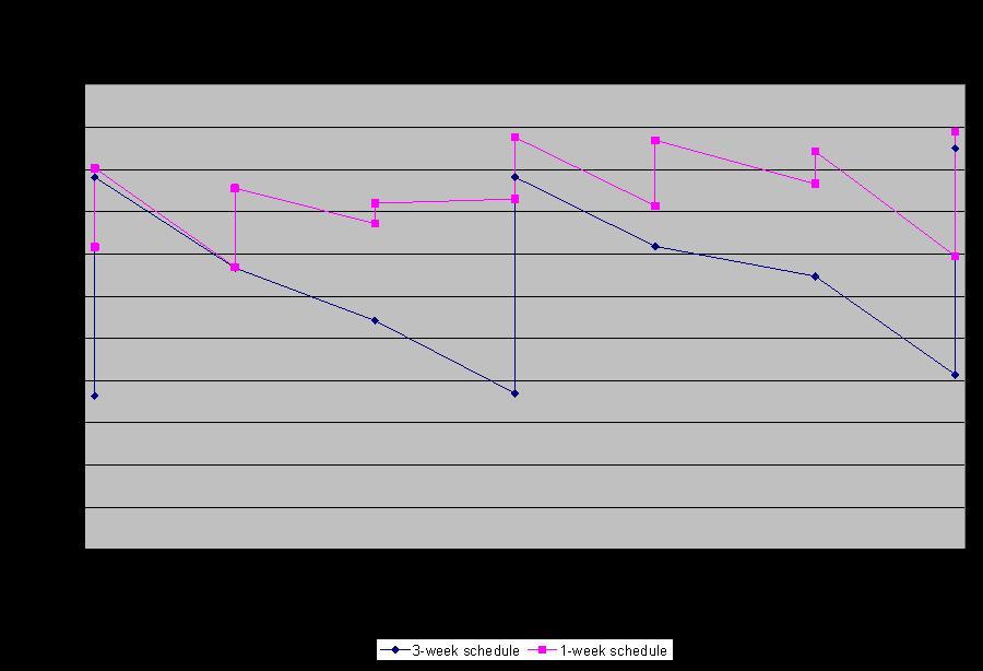
66 Information Decay

67 Dynamic Portfolio Selection Consider the following infinite horizon utility maximization problem: X max E" γ t u(µ t, x t) {x t } t=0,... t=0 where γ is a discount factor, and u( ) is the utility function we have seen before: u(µ, x) = µ T x λx T Σx φtc(t) T t. For simplicity, we assume TC(t) = Λt and ignore constraints for now. Also assume the following mean-reverting model for expected returns: µ t = (I β)µ t 1 + β µ + ε t where β is a diagonal matrix of mean reversion coefficients and µ is the vector of average expected returns. ε is white noise. Σ and Λ are time-invariant. Different factors will have different mean reversion rates. This is important for trading costs. #

68 Dynamic Portfolio Selection Consider the following infinite horizon utility maximization problem: X max E" γ t u(µ t, x t) {x t } t=0,... t=0 where γ is a discount factor, and u( ) is the utility function we have seen before: u(µ, x) = µ T x λx T Σx φtc(t) T t. For simplicity, we assume TC(t) = Λt and ignore constraints for now. Also assume the following mean-reverting model for expected returns: µ t = (I β)µ t 1 + β µ + ε t where β is a diagonal matrix of mean reversion coefficients and µ is the vector of average expected returns. ε is white noise. Σ and Λ are time-invariant. Different factors will have different mean reversion rates. This is important for trading costs. #

69 Dynamic Portfolio Selection Consider the following infinite horizon utility maximization problem: X max E" γ t u(µ t, x t) {x t } t=0,... t=0 where γ is a discount factor, and u( ) is the utility function we have seen before: u(µ, x) = µ T x λx T Σx φtc(t) T t. For simplicity, we assume TC(t) = Λt and ignore constraints for now. Also assume the following mean-reverting model for expected returns: µ t = (I β)µ t 1 + β µ + ε t where β is a diagonal matrix of mean reversion coefficients and µ is the vector of average expected returns. ε is white noise. Σ and Λ are time-invariant. Different factors will have different mean reversion rates. This is important for trading costs. #

70 Finite Horizon Formulation The finite-horizon recursion for the problem is given by: J N (µ N, x N 1 ) = max t N (x Nµ N λx NΣx N φt NΛt N ) J t (µ t, x t 1 ) = max t t E [x tµ t λx tσx t φt tλt t + γj t+1 (µ t+1, x t )] Period N problem is a simple QP. Solving it, we obtain: t N = 1 2 (λσ + φλ) 1 µ N (λσ + φλ) 1 (λσ) x N 1

71 Finite Horizon Formulation The finite-horizon recursion for the problem is given by: J N (µ N, x N 1 ) = max t N (x Nµ N λx NΣx N φt NΛt N ) J t (µ t, x t 1 ) = max t t E [x tµ t λx tσx t φt tλt t + γj t+1 (µ t+1, x t )] Period N problem is a simple QP. Solving it, we obtain: t N = 1 2 (λσ + φλ) 1 µ N (λσ + φλ) 1 (λσ) x N 1

72 The Value Function Define the following matrices: A N B N = 1 2 (λσ + φλ) 1 = (λσ + φλ) 1 (λσ) so that t N = A N µ N B N t N 1 Then, J N (µ N, t N 1 ) = µ NM N µ N + x N 1N N x N 1 + x N 1P N µ N where M N = 1 2 A N N N = φλb N P N = 2φΛA N

73 The Value Function Define the following matrices: A N B N = 1 2 (λσ + φλ) 1 = (λσ + φλ) 1 (λσ) so that t N = A N µ N B N t N 1 Then, J N (µ N, t N 1 ) = µ NM N µ N + x N 1N N x N 1 + x N 1P N µ N where M N = 1 2 A N N N = φλb N P N = 2φΛA N

74 Recursion Given the shape of J N ( ), we hypothesize that J t ( ) will be quadratic and try to solve for the coefficients of this quadratic model. Indeed, J t ( ) = µ tm t µ t + x t 1N t x t 1 + x t 1P t µ t + q tµ t + r tx t 1 + f t τ t = A t µ t B t x t 1 + c t for certain parameters A t, B t, etc., derived from Σ, Λ, β, etc. An infinite horizon extension is relatively straight-forward and requires the solution of a fixed-point problem.

75 Recursion Given the shape of J N ( ), we hypothesize that J t ( ) will be quadratic and try to solve for the coefficients of this quadratic model. Indeed, J t ( ) = µ tm t µ t + x t 1N t x t 1 + x t 1P t µ t + q tµ t + r tx t 1 + f t τ t = A t µ t B t x t 1 + c t for certain parameters A t, B t, etc., derived from Σ, Λ, β, etc. An infinite horizon extension is relatively straight-forward and requires the solution of a fixed-point problem.

76 How do we use this for constrained problems? We use our knowledge of J( ) to set up a quadratic program which will approximate the optimal solution to the constrained multi-period rebalancing problem. The QP is then given by: max t t s.t. which is equivalent to x t µ t λx t Σx t φt tλt t + γe [J (µ t 1, x t 1 + t t)] x t = x t 1 + t t X max t t λσ + φλ γn tt + µ t + 2 (λσ γn) x t t 1+ t γp ((I β)µ t + β µ) + γr t t s.t. x t = x t 1 + t t X

77 Alternatives Can we construct one-period problems that partially capture the dynamics of the inputs? For example, incorporate the decay rate into the expected returns used in optimizations. One critical issue is the selection of the t-cost aversion parameter φ. It needs to balance the expected return rates with the trading costs, so the aversion parameter must ensure that these terms are in the same units. But this creates a chicken-and-egg problem.

78 Alternatives Can we construct one-period problems that partially capture the dynamics of the inputs? For example, incorporate the decay rate into the expected returns used in optimizations. One critical issue is the selection of the t-cost aversion parameter φ. It needs to balance the expected return rates with the trading costs, so the aversion parameter must ensure that these terms are in the same units. But this creates a chicken-and-egg problem.

79 Alternatives Can we construct one-period problems that partially capture the dynamics of the inputs? For example, incorporate the decay rate into the expected returns used in optimizations. One critical issue is the selection of the t-cost aversion parameter φ. It needs to balance the expected return rates with the trading costs, so the aversion parameter must ensure that these terms are in the same units. But this creates a chicken-and-egg problem.

80 Consistent t-cost aversion u(µ, x) = µ T x λx T Σx φtc(t) T t. If µ is an annualized return estimate, and TC(t) T t is a one-time trading-cost, to bring these two terms to comparable units, φ must correspond to the expected number of trades per year for the securities in the portfolio. The problem is, for lower φ, we have higher turnover and higher expected number of trades per year perhaps inconsistent with the φ we used. Similar problem for φ that is too high. How do we find the right value of this parameter? Iterate to achieve consistency...

81 Consistent t-cost aversion u(µ, x) = µ T x λx T Σx φtc(t) T t. If µ is an annualized return estimate, and TC(t) T t is a one-time trading-cost, to bring these two terms to comparable units, φ must correspond to the expected number of trades per year for the securities in the portfolio. The problem is, for lower φ, we have higher turnover and higher expected number of trades per year perhaps inconsistent with the φ we used. Similar problem for φ that is too high. How do we find the right value of this parameter? Iterate to achieve consistency...

82 Consistent t-cost aversion u(µ, x) = µ T x λx T Σx φtc(t) T t. If µ is an annualized return estimate, and TC(t) T t is a one-time trading-cost, to bring these two terms to comparable units, φ must correspond to the expected number of trades per year for the securities in the portfolio. The problem is, for lower φ, we have higher turnover and higher expected number of trades per year perhaps inconsistent with the φ we used. Similar problem for φ that is too high. How do we find the right value of this parameter? Iterate to achieve consistency...

83 Recap Trading costs are important considerations for asset managers. Optimization tools are crucial in managing these costs carefully. Trading multiple accounts simultaneously poses a difficult question of balancing optimality and fairness. An equilibrium approach seems best suited for this situation. Conic optimization tools are essential. Dynamic programming and optimal control techniques are useful in addressing the multi-period portfolio selection models. However, computational burden is still too high for a true solution of this problem. Instead, we focus on informed heuristics.

84 Recap Trading costs are important considerations for asset managers. Optimization tools are crucial in managing these costs carefully. Trading multiple accounts simultaneously poses a difficult question of balancing optimality and fairness. An equilibrium approach seems best suited for this situation. Conic optimization tools are essential. Dynamic programming and optimal control techniques are useful in addressing the multi-period portfolio selection models. However, computational burden is still too high for a true solution of this problem. Instead, we focus on informed heuristics.

85 Recap Trading costs are important considerations for asset managers. Optimization tools are crucial in managing these costs carefully. Trading multiple accounts simultaneously poses a difficult question of balancing optimality and fairness. An equilibrium approach seems best suited for this situation. Conic optimization tools are essential. Dynamic programming and optimal control techniques are useful in addressing the multi-period portfolio selection models. However, computational burden is still too high for a true solution of this problem. Instead, we focus on informed heuristics.

86 Additional information 1 This material is provided for educational purposes only and should not be construed as investment advice or an offer or solicitation to buy or sell securities. 2 THIS MATERIAL DOES NOT CONSTITUTE AN OFFER OR SOLICITATION IN ANY JURISDICTION WHERE OR TO ANY PERSON TO WHOM IT WOULD BE UNAUTHORIZED OR UNLAWFUL TO DO SO. 3 These examples are for illustrative purposes only and are not actual results. If any assumptions used do not prove to be true, results may vary substantially. 4 The opinions expressed in this research paper are those of the authors, and not necessarily of GSAM. The investments and returns discussed in this paper do not represent any Goldman Sachs product. This research paper makes no implied or express recommendations concerning how a clients account should be managed. This research paper is not intended to be used as a general guide to investing or as a source of any specific investment recommendations. 5 Opinions expressed are current opinions as of the date appearing in this material only. No part of this material may, without GSAMs prior written consent, be (i) copied, photocopied or duplicated in any form, by any means, or (ii) distributed to any person that is not an employee, officer, director, or authorised agent of the recipient. 6 Copyright c 2007, Goldman, Sachs Co. All rights reserved.