Mathacle. PSet Stats, Concepts In Statistics Level Number Name: Date: Distribution Distribute in anyway but normal

Transcription

1 Distribution Distribute in anyway but normal VI. DISTRIBUTION A probability distribution is a mathematical function that provides the probabilities of occurrence of all distinct outcomes in the sample space. There are several important probability distributions: binomial distribution, normal distribution, t-distribution, chi-squares distribution, F distribution and Poisson distribution. The t-distribution, chi-squares distribution and F distribution are related to gamma functions. The Poisson distribution and F distribution are not tested in the AP Exam. 6.. The Discrete Random Variable and Its Probability Distribution [MATH] A discrete random variable is a function X : F Ω, where a mapping from the event space to real numbers. Ω R. That is, it is 08

2 Example 6... Toss of a fair die twice. Find the sample space and the random variable X that is defined as the sum of the two outcomes. The sample space is Ω = { (, ), (, ),, ( 6,6) } the two outcomes is X {, 3,,}.. The random variable that is the sum of [MATH] The probability density function (pdf) or probability mass function (pmf) of a discrete random variable X is a non-negative function p : R [0, ], defined by x R p ( x) = P( X = x), for x R and it satisfies p ( x) =. p (x) is sometimes referred to as the probability distribution function. The cumulative distribution function (cdf) of a discrete variable X is a non-decreasing, right-continuous function F : R [0, ], defined by and it satisfies F( ) = 0 and F ( ) =. F ( x) = P( X x) = p( x ), for x R x x i i 09

3 F (x) has the following properties:.) If x y, then F( x) F( y).) P( a < x b) = P( X b) P( X a) = F( b) F( a) Example 6... Toss of a fair coin three times. Let X be the random variable that counts the number of Heads up. Find the sample space and the probability density function p (x). The sample space is Ω = { HHH, HHT,, TTT} random variable X {0,,, 3}.. The number of Heads showing up is a Ω HHH HHT HTH THH HTT THT TTH TTT X 3 0 The pdf p(x) and cdf F(x) are X 0 3 p (x) F (x) The distribution is a binomial probability distribution with probability of 0.5 and size of 3: 0

4 [MATH] Let X and X be two independent integer-valued random variables, with distribution functions p ( x) and p ( x) respectively, and Y = X + X be the sum of the two variables. The distribution of Y is the convolution of p ( ) and p ( ) given by x x For j =...,,, 0,,,,... p ( j) p ( k) p ( j y = k k ) For example, a die is rolled twice. Let X and X be the outcomes, and let Y = X + X be the sum of these outcomes. Then and Etc. p y ( p y ) = p () p () = 36 ( 3) = p () p () + p() p () = p ( x) = p ( x) = for x {,,3,4,5,6 }, 6 36 p y ( 4) = p () p (3) + p () p () + p(3) p () = 3 36

5 Example You roll a pair of dice. Let Y be the sum of rolling two dice. Calculate and sketch the PDF of Y if they are a pair of fair dice? x p y (x) This is an equally likely event problem. D\D

6 Example [MC035M] An urn contains exactly three balls numbered,, and 3, respectively. Random samples of two balls are drawn from the urn with replacement. X + X The average, X =, where X and X are the numbers on the selected balls, is recorded after each drawing. a.) Describe the probability distribution of X? X p ( X ) F ( X ) b.) If you draw two balls and the average X =, do you think that the outcome is significant (or rare)? 3

7 a.) This is an equally likely event problem as the outcomes are equally likely. The random variables are the numbers X {,,3 } and X {,,3 }, and the averages X + X X = are: X \ X 3 X \ X p ( X ) F ( X ) b.) P ( X = ) = %. The result is not significant because the probability is too high. 4

8 Quick-Check Discrete Random Variables and Probability Functions QC 6... For a monthly subscription fee, a video download site allows people to download and watch up to five movies per month. Based on past download histories, the following table gives the estimated probabilities that a randomly selected subscriber will download 0,,, 3, 4 or 5 movies in a particular month. # of downloads Estimate Probability If a subscriber is selected at random, what is the estimated probability that is subscriber downloads a.) three or fewer movies b.) at least three movies c.) four or more movies d.) zero or one movies e.) more than one movies QC 6... [MC0738M] A game of chance is played in which X, the number of points scored in each game, has the distribution shown below. Calculate and sketch the PDF and CDF of the sampling distribution of the sum of the scores Y when the game is played twice. Write your answers in decimal numbers. 5

9 Answers QC 6... a.) 0.83, b.) 0.7, c) 0.7, d.) 0.48, e.) 0.5 QC 6... Let the random variable Y = X + X. Assume that the each game played is independent from the next. That is, P ( X X ) = P X ) P( ). ( X X / P (Y ) \ X Y Event X + X p (y) F (Y )

10 6.. The Expected Value, Standard Deviation and Variance [MATH] The mathematical expectation of a discrete variable X, or just mean of X, is defined as E [ X ] = x p( x) The alternative notation µ (X ), or just µ, are often used. The expectation of a continuous random variable X, is defined as E[ X ] xp( x) dx = For any constant c and d, random variables X and Y :.) E [ cx ] = c x p( x) = c x p( x) = ce[ X ].) E [ cx + d] = ( cx + d) p( x) = c x p( x) + d p( x) = ce[ X ] + d 3.) E [ X + Y ] = E[ X ] + E[ Y ] Proof: E[ X + Y ] = ( x + y) p( x, y) = xp( x, y) + yp( x, y) = xp( x) + yp( y) = E[ X ] + E[ Y ] 0

11 4.) E[ XY ] = E[ X ] E[ Y ], if random variables X and Y are independent. Proof: xyp( x, y) = xyp( x) p( y) = xp( x) yp( y) = E [ XY ] = E[ X ] E[ Y ] Example 6... Toss of a fair coin three times. Find the expected value for the number of heads showing up. Let the random variable X be the number of Heads. Then, X 0 3 p (x) E [ X ] = xp( x) = = This means when the experiment repeats a large number of times, the average number of Heads showing up is.5. Be careful with addition of random variables. For example, if the random variable of the weight for an apple is X, the random variable of the weight of five apples is not 5X, but X + X + X + X + X

12 Example 6... [CB] In a certain game, a fair die is rolled and a player gains 0 points if the die shows a 6. If the die does not show a 6, the player loses 3 points. If the die were to be rolled 00 times, what would be the expected total gain or loss for the player? Let the random variable X be the points a player gains when the die is rolled once. Then X 0-3 p (x) E 5 5 [X ] 0 3 = X i i= The expected value of Y = for rolling 00 times of the die is E[ Y ] = E X = [ ] = i E X i E[ X ] = 00 E[ X ] = i= i= i= 6 Example In a game, a fair die is tossed once. If the number of spots showing is either 4 or 5, you win $. If the number of spots showing is 6, you win $4. If the number of spots showing is, or 3, you win nothing. It costs you $ to play a game. If the die were to be rolled 00 times, what would be the expected total gain or loss for you? Number on die,, 3 4, 5 6 X $0 $ $4 p (x) E [X ] = 6 6 6

13 The expected value of total gain/loss of Y = E[ Y ] = E[ X i 00] = E[ X i= i= 00 X i i= i 00 is ] 00 = 00 E[ X ] 00 = 0 [MATH] The expected value of any real-valued function g( x) is defined as E[ g( X )] = g( x) p( x) n When g( x) = x, the expected value of g( x) is the th n moment of X n n E[ g( X )] = E[ X ] = x p( x) The mean is the st moment of X. The variance of a discrete variable X is expected value of g( X ) = ( X E[ X ]) : ( X E[ X ]) ] = ( x E[ X ]) Var [ X ] = E[ g( X )] = E[ p( x) The alternative notation ( X σ ), or just σ, are often used. The quantity σ = Var[ X ], the positive square root of the variance, is the standard deviation of X. Example Roll a fair die once. Find the expected value and variance of the number facing up. The expected value of the number facing up is 7 E [ X ] = =

14 The variance is x (x) p ( x E[ X ]) /6 5/4 /6 9/4 3 /6 /4 4 /6 /4 5 /6 9/4 6 /6 5/ Var [ X ] = = [MATH] For any constant c and d,.) Var[ X ] = E[ X ] ( E[ X ] ) Proof: Var[ X ] = = = = E[ X ( x E[ X ]) p( [ X ] + ( E[ X ]) ( x xe ) p( x) ( x ) p( x) E[ X ] x p( x) + ( E[ X ]) ] ( E[ X ]) x) p( x).) Var[ cx + d] = c Var[ X ] 4

15 Proof: Var[ cx + d] = = E[ c = c X = c E[ X + ] + E[ ( cx + d ) ] ( E[ cx + d] ) cdx + d ] ( ce[ X ] + d ) cde[ X ] + d ( ce[ X ] + d ) ( E[ X ]) ( E[ X ] ) = c Var[ X ] If random variables X and Y are independent, then 3.) Var[ X ± Y ] = Var[ X ] + Var[Y] Example Find the mean and variance for the pdf of X given by p x = 0 p( x) = p x = 0 otherwise E[ X ] = 0 ( p) + p = p E[ X ] = 0 ( p) + p = p ( ) Var[ X ] = E[ X ] E[ X ] = p p Example LetY = 800X 900, where the pdf of X is given by Find the mean and variance of X and Y. x 3 4 p( x )

16 E[ X ] = (0.) + (0.) + 3(0.3) + 4(0.4) = 3 E[ X ] = (0.) + (0.) + 3 (0.3) + 4 (0.4) = 0 Var[ X ] = E[ X ] ( E[ X ]) = 0 3 = E[ Y ] = E[800X 900] = 800 E[ X ] 900 = 800(3) 900 = 500 Var[ Y ] = Var[800X 900] = 800 Var[ X ] = 800 Example Let Y X X = , where the pdf of X is given by Find expected values of X and Y. x p( x ) E [ X ] = 4(0.5) + 6(0.3) + 8(0.) = 5.4 E [ Y ] = 40(0.5) + 56(0.3) + 76(0.) = 5 y p( y ) Example Flip a dice twice and let X be the sum of the two outcomes. X is a discrete random variable, a.) Find the pdf function of X b.) Use pdf to compute P( X 4), P( X < 4) and P( X 4) 6

17 c.) Compute the cumulative distribution function (cdf) of X. x p( x ) d.) Use cdf to compute P( X 4), P( X < 4) and P( X 4) e.) Compute E[ X ], Var[ X ] and σ = Var[ X ] x a.) x p( x ) / 36 / 36 3 / 36 4 / 36 5 / 36 6 / 36 5 / 36 4 / 36 3 / 36 / 36 / 36 b.) c.) 6 P( X 4) = p() + p(3) + p(4) = 36 3 P( X < 4) = p() + p(3) = P( X 4) = ( p() + p(3) ) = 36 7

18 d.) e.) 6 P( X 4) = F(4) F() = 36 3 P( X < 4) = F(3) F() = P( X 4) = F(3) = 36 E[ X ] = = E X = = [ ] Var X = E X E X = = [ ] [ ] ( [ ]) σ = Var[ X ] = 5.83 =.4 x 8

19 Quick-Check 6... The Expected Value, Standard Deviation and Variance QC 6... [CB] The Attila Barbell Company makes bars for weight lifting. The weights of the bars are independent and are normally distributed with a mean 70 ounces and a standard deviation of 4 ounces. The bars are shipped 0 in a box to the retailers. The weights of the empty boxes are normally distributed with a mean of 30 ounces and a standard deviation of 8 ounces. The weights of the boxes filled with 0 bars are expected to be normally distributed. What are the mean and standard deviation of the weights of the filled boxes? QC 6... You buy a racehorse for $0,000, and enter it in two races. You plan to sell the horse afterward, hoping to make a profit. If the horse wins both races, its value will jump to $00,000. If it wins one of the races, it will be worth $50,000. If it loses both races, it will be worth only $0,000. It is believed that there is a 40% chance that the horse will win the first race and a 30% chance it will win the second one. It is also believed those two races are independent events. Let X be the random variable of profit from sale of the horse. a.) What are the mean, standard deviation and variance of X? b.) Suppose the horse values all of a sudden quadruple. What is the mean, standard deviation and variance of new random variable Y = 4X? c.) Suppose you miscalculated the horse values, and all values should be increased by $0,000. What is the mean, standard deviation and variance of new random variable Z = X ? 9

20 Answers QC 6... Assume the following random variables: W = weight of a bar B = weight of a box Then, the random variable of a box filled with ten bars is So, the mean is Y = B + 0 W i i= 0 0 E[ Y ] = E[ B + Wi ] = E[ B] + E[ Wi ] = E[ B] + 0E[ W ] = (70) = 750 i= and standard deviation is i= 0 Var [ Y ] = Var[ B + Wi ] = Var[ B] + Var[ Wi ] = 0 i= i= 8 + 0(4 ) = 4 QC 6... a.) The probabilities for each case are expressed in the two-way table and the tree diagram: Event LL WL+LW WW X 0, ,000 80,000 P( X = x)

21 E[ X ] = 0000(0.4) (0.46) (0.) = 900 ( ) E X = + + = [ ] 0000 (0.4) (0.46) (0.) ( ) Var X = E X E X = [ ] [ ] [ ] σ = Var[ X ] = 946 x b.) ( ) E[ Y ] = E[4 X ] = 4 E[ X ] = = Var[ Y ] = Var[4 X ] = 6 Var[ X ] = σ = Var[ Y ] = 4σ = 6984 y c.) x E[ Z] = E[ X ] = E[ X ] = 900 Var[ Z] = Var[ X ] = Var[ X ] = σ = Var[ Z] = σ = 946 z x 3

22 6.3. The Binomial Distribution and the Geometrical Distribution In life, there could be three options. Binomial Distribution The Bernoulli Processes are based on the following assumptions (BINS):.) B Each trial has only two possible outcomes: success or failure, and the two outcomes are mutually exclusive..) I The trials are independent. 3.) N There are countable n trials 4.) S The probability of success, denoted by p, is the same for each trial. The probability of failure is p, and is also the same for each trial. The random variable X describing Bernoulli trials often takes value of one for the success and the value of zero for the failure for each trial. Example A student writes a five-question multiple-choice quiz. Each question has four possible responses. The student guesses at random for each question. The random variable X is the number of correct answers the student gets. Do the results form a sequence of Bernoulli trials? Yes, they are Bernoulli trials as the BINS are satisfied: B: correct or incorrect. So, B is defined. I: each question (trial) is independent of the others. I is fine. 35

23 N: n = 5, the number is countable. S: all guesses have the same one fourth of chance to be correct. S is satisfied. Example An auto manufacturer chooses one car from each hour s production for a detailed quality inspection. The random variable X is the number of cars having paint defects. Do the inspection results form a sequence of Bernoulli trials? No, the condition N fails: B: yes, or no, so B is defined. I: all inspections are independent, so I is fine. N: no N. It would be fine if the auto manufacturer does inspection for a specific number of hours. S: all cars have the same probability of having defects in paints. S is satisfied. Example The pool of potential jurors for a murder case contains 00 persons chosen at random from adult residents of a large city. Each person is asked whether he or she opposes the death penalty. The random variable X is the number of people who say Yes. Do the results form a sequence of Bernoulli trials? Yes. B: yes or no. B is fine. I: all responses are independent. I is fine. N: n = 00, N is countable. S: Assume all have the same probability of saying yes. S is satisfied. 36

24 For each trial, a binomial random variable X is assigned to be for a success outcome and 0 for a failure outcome. That is, P( X = ) = p and P( X = 0) = p If X is the sum of n independent random binomial variables, each of which has the same the success probability p : X = X + X X n then the mean of X is E X ] = E[ X ] + E[ X ] E[ X ] [ = p + p p = np and the variance of X is Var[ X ] = Var[ X] + Var[ X ] Var[ X n ] = p( p) + p( p) p( p) ( p) = np n 37

25 [MATH] The binomial random variable X that counts x successes in n independent trials has the binomial distribution b( n, p, x ) with same success probability p in each trial. The probability of P( X = x) is given by for x { 0,,,..., n} x P( X = x) = b( n, p, x) = C p ( p) x P( X x) b( n, p, i) = i= 0. The mean or the mathematical expectation of X is µ = np and its standard deviation is σ = np( p). n x n x [Ti-84] and P( X = x) = b( n, p, x) = binompdf ( n, p, x) x P( X x) = b( n, p, i) = binomcdf ( n, p, x) i= 0 Example A bag contains 4 red balls and 3 green balls. If a ball is picked up and put back randomly for 5 times, what is the probability when i. the first two balls are red and the next 3 balls are green? ii. the odd picks are red balls and the even picks are blue balls? The probability of picking a red is 4 p = and the probability of picking a green is i. P( st two red balls ) = p p q q q = = q =, so 7 38

26 3 4 3 ii. P( odd red and even blue ) = p q p q p = = Example A biased trade dollar is tossed 6 times. The probability of heads on any toss is about Let the random variable X denotes the number of heads that come up. i. What is the probability of exactly two heads up? ii. What is the probability of getting at least two heads and no more than five heads? The probability of picking a head is p = 0. 3 and the probability of picking a tail is q = i. The probability of exactly two heads up is P ( X = ) = b(6, 0.3, ) = = 6 6 C C p 0.34 q 4 ( 0.3) ( 0.3) ii. The probability of getting at least two heads and no more than five heads is 6 or P ( < X 5) = b(6, 0.3, ) + b(6, 0.3, 3) + b(6, 0.3, 4) + b(6, 0.3, 5) 5 6 x 6 x = ( 0.3) ( 0.7) x= x =

27 ( ) P < X 5 = P( X 5) P( X ) = binomcdf (6, 0.3, 5) binomcdf (6, 0.3,) = Example Suppose that Jon guesses on each question of a 50-item true-false quiz. Find the probability that Jon passes if a score of 30 or more is needed to pass. ( ) P X 30 = P( X 9) = binomcdf (50, 0.5, 9) = 0.0 Example [MC40] The probability of winning a certain game is 0.5. If at least 70 percent of the games in a series of n games are won, the player wins a prize. If the possible choices for n are n = 0, n = 0, and n = 00, which value of n should the player choose in order to maximize the probability of winning a prize? for each game, p = 0.5, q = At least 70 percent of winning means to find P( X 70%) for each given n : For n = 0 : P( X = 0 C 70%) ( 0.5) ( 0.5) + C ( 0.5) ( 0.5) + C ( 0.5) ( 0.5) + C ( 0.5) ( 0.5) 0 = binomcdf (0,0.5,6)

28 For n = 0 : P( X 70%) = binomcdf (0,0.5,3) For n = 00 : The answer is n = 0. P( X 70%) = binomcdf (00,0.5,69) Example A multiple-choice quiz contains questions with 3 possible answers. If someone guesses on every answer, what is the probability of getting more answers correct than it would have been expected by chance? p = and n =. The mean or expected value of number of getting it correct is 3 µ = np = = 4. P ( X > 4) = binormcdf (, / 3, 4) = Binomial PDF The sum of all the binomial probabilities: n n x= 0 m= 0 n ( ) x n x P( X = x) = C p ( p) = p + ( p) = x The following graphs show the binomial distributions b( n, p, x ) for some given n and p when x { 0,,,..., n}. Case #: p = 0. 5 n 4

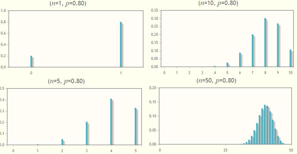
29 Case #: p = 0. Case #3: p =

30 The distribution is symmetric when p = 0. 5 ; the distribution is skewed to the left when p > 0.5, and finally the distribution is skewed to the right when p < 0.5. Geometric Distribution A random variable X is a geometric random variable of trials if the following conditions are satisfied (BITS): I. B Each trial has only two possible outcomes: success or failure, and the two outcomes are mutually exclusive. II. I The trials are independent. III. T The experiment consists of repeating trials until the first success IV. S The probability of success, denoted by p, is the same for each trial. The probability of failure is p, and is also the same for each trial. The random variable X is the number of trials. The pdf of X is given by x P( X = x) = g( p, x) = q p [MATH] The cumulative probability function of X is given by F( x) = P( X x) = P( X = ) + P( X = p + qp + q = p( + q + q x q = p q = q x p q q x x ) p = ) + + P( X = x) The mean of X is 43

31 E[ X ] = = = p p x= x xq x= 3 ( + q + 3q + 4q + ) = p The proof of variance is a little complicated and the formula can be easily driven by applying the derivatives: q Var [ X ] = E[ X ] ( E[ X ]) = p xq x p [ Ti-84] g( p, x) = geometpdf ( p, x) x P( X x) = g( p, i) = geometcdf ( p, x) i= Example Flip a coin until you observe a tail. Determine if the experiment describes a geometric distribution. Yes. B: Only two choices, head and tail I: Each flip is independent T: Flip until you observe a tail S: Probability of success is the same each as p =

32 Example There are 0 red marbles and 5 blue marbles in a jar. You reach in randomly to select a marble. You want to know how many marbles you will have to draw, without replacement, in order to be sure that you have 3 red marbles on average. Determine if the experiment describes a geometric distribution. No. B: Only two choices, red and blue I: Each selection is NOT independent T: It is not looking for the first success S: Probability of success varies for each selection Example A student is randomly generating one-digit numbers. What is the probability that the first 4 will be the 8 th digit generated? Let X be the number of times to generate a one-digit number. Then or P X 7 ( ) ( ) 7 ( = 8) = q p = P( X = 8) = geometpdf (0.,8) Example The color distribution in a bag of Reese s Pieces was found to be 3 brown, orange, and 5 yellow. If one piece is randomly drawn and replaced, what is the probability that it will take less than 8 draws to get an orange piece? Let X be the number to draw to get an orange piece. Then, 45

33 or 7 7 i 7 ( 7) = (0.44, ) = (0.56) (0.44) = P X g i i= i= P( X 7) = geometcdf (0.44, 7) Example A recent study at THS finds that 3% of seniors have taken ACT only. What is the average number of seniors you would ask to find out one senior who took ACT only? Let X be the number of times to ask seniors. Then E[ X ] = 3.3 p = 0.3 Example Mr. THS is the only receiver of the football team with the likelihood of catching a pass of 0.5. Solve each question and indicate if it is binomial or geometric. Let X be the number of passes caught and let Y be number of passes to have the first pass caught. a.) What is the probability that passes are caught out of 6 passes? b.) What is the probability that no passes are caught out of 6 passes? c.) What is the probability that first pass caught on the st pass? d.) What is the probability that or fewer passes are caught out of 6 passes? 46

34 e.) What is the probability that more than passes are caught out of 6 passes? f.) What is the probability that first pass is on the 4 th pass? g.) What is the probability that the first pass is caught within first 3 attempt? h.) What is the probability that the first pass is caught after first 3 attempts? i.) What is the expected number of catches with 6 attempts? j.) What is the expected number of attempts for the first pass caught? a.) Binomial, b.) Binomial, P X b C 4 ( = ) = (6, 0.5, ) = 6 (0.5) ( 0.5) 0.76 P X b C 0 6 ( = 0) = (6, 0.5, 0) = 6 0(0.5) ( 0.5) c.) Geometric, d.) Binomial, P Y ( = ) = g(0.5,) = ( 0.5) (0.5) 0.5 i 6 i ( ) = (6, 0.5, ) = 6 i (0.5) ( 0.5) i= 0 i= 0 P X b i C 47

35 e.) Binomial, P( X > ) = P( X ) = f.) Geometric, g.) Geometric, P Y 4 ( = 4) = g(0.5, 4) = ( 0.5) (0.5) i ( 3) = (0.5, ) = ( 0.5) (0.5) P Y g i i= i= h.) Geometric, P( Y > 3) = P( X 3) = i.) Binomial, E[ X ] = np = 6(0.5) = 0.9 j.) Geometric, E[ Y ] = p = 0.5 = Example Miss Archer Columbia is able to hit the bull s eye 80% of the time. Assume that each shot is independent of the others. Miss Archer Columbia shoots 6 arrows. Let X be the number of bull s eye hit, and let Y be the number of shots needed to have the first bull s eye hit. Find the probability in each of following cases: a.) Her first bull s eye comes on the 3 rd arrow. b.) She misses the bull s eye at least once. c.) Her st bull s eye comes on the 4 th or 5 th arrow. d.) She gets exactly four bull s eyes. e.) She gets at least four bull s eyes 48

36 f.) She gets at most four bull s eyes g.) How many bull s eyes do you expect her to get? h.) What is the standard deviation? i.) If she keeps shooting arrows until she hits the bull s eye, how many times do you expect her to hit the bull s eye? p = 0.8, q = 0., the pdf of X for binomial is X P( X = x) 6 q 0 b(6, 0.8,) b(6,0.8, ) b(6, 0.8,3) b(6,0.8, 4) b(6, 0.8,5) p 0.6 a.) Geometric, P Y 3 ( = 3) = g(0.8, 3) = ( 0.8) (0.80) = 0.03 b.) Binomial, P( X < 6) = P( X = 6) 0.6 = c.) Geometric, (( = 4) ( = 5) ) P Y Y = g(0.8, 4) + g(0.8,5) = ( 0.8) (0.80) ( 0.8) (0.80) = d.) Binomial, P( X = 4) = 0.458, from the above table 49

37 e.) Binomial, from the above table. f.) Binomial, from the above table. P( X 4) = P( X = 4) + P( X = 5) + P( X = 6) = = 0.90 P( X 4) = P( X = 5) P( X = 6) = = g.) Binomial, E[ X ] = np = 6(0.8) = 4.8 h.) Binomial, σ x = Var[ X ] = np( p) = 6(0.8)( 0.8) = i.) Geometric, E[ Y ] =.5 p = 0.8 = Example [FRQB03] An airline claims that there is a 0.0 probability that coach-class ticket holder who flies frequently will be upgraded to first class on any flight. This outcome is independent from flight to flight. Sam is a frequent flier who always purchases coach-class tickets. (a) What is the probability that Sam s first upgrade will occur after the third flight? (b) What is the probability that Sam will be upgraded exactly times in his next 0 flights? (c) Sam will take 04 flights next year. Would you be surprised if Sam receives more than 0 upgrades to first class during the year? Justify your answer. 50

38 a.). b.) P ( X c.) It is very unlikely. P( X 4) ( P X P X P X ) = ( = ) + ( = ) + ( = 3) = + + (0. 0.9(0.) 0.9 (0.)) = = ) = binompdf 8 ( 0.) ( 0.9) = (0,0.,) P( X > 0) = binomcdf (04, 0., 0)

39 Quick-Check The Binomial and the Geometric Distributions QC students of THS are in AP Stats class. After completing their study, all students take the AP exam. Assume the random variable is the number of students who receive a 4 or higher. Do the results form a sequence of Bernoulli trials? QC Each child in Dalal family has ¼ of having blood type O. Suppose there are five children in the family, what is the probability that exactly two children have type O blood? QC An airline has an on-time arrival rate of 8.4%. What is the probability that if you travel on this airline, no more than of your next 0 flights will not be on time? (A) ( 0.76) ( 0.84) + ( 0.76) ( 0.84) + ( 0.76) ( 0.84) (B) ( ) ( ) ( ) ( ) ( ) ( ) (C) ( ) ( ) ( ) ( ) (D) ( ) ( ) (E) ( ) ( ) 5

40 QC [MC07] Julie generates a sample of 0 random integers between 0 and 9 inclusive. She records the number of 6 s in the sample. She repeats this process 99 more times, recording the number of 6 s in each sample. What kind of distribution has she simulated? (A) The sampling distribution of sample proportion with n = 0 and p = 6 (B) The sampling distribution of sample proportion with n = 00 and p = 0. (C) The binomial distribution with n = 0 and p = 0. (D) The binomial distribution with n = 00 and p = 0. (E) The binomial distribution with n = 0 and p = 0. 6 QC About 77% of Americans claim to always recycle. Suppose that people are randomly surveyed and asked whether they always recycle. What is the probability that between 5 and 8 people inclusive say no? (A) (B) (C) (D) (E) QC It is known that screws produced by a certain company will be defective with probability 0.0, independently of each other. The company sells the screws in packages of 0 and offers a money-back guarantee that at most of the 0 screws is defective. What proportion of packages sold must the company replace? QC A random digit generator is set to generate random digits between 0 and 9. What is the probability that at least 6 of the digits generated are greater than 3? 53

41 QC In a 007 study, it was reported that 6% of American public thought of themselves as chronic procrastinators. Suppose this percentage has not changed. If 00 Americans are randomly surveyed, what is the mean and standard deviation of the number who will say they are chronic procrastinators? QC Which of the following statements is NOT correct?. (A) The number of successes that corresponds to the maximum value of a binomial PDF is within one unit of its mean. (B) A geometric PDF is always decreasing. (C) A binomial PDF with p < 0.5 will be skewed right. (D) As the number of trials in a geometric situation increases and the number of successes in a binomial situation increases, the value of CDF approaches to zero. (E) A PDF can be transformed by using addition. QC Sixty-five percent of all divorce cases cite incompatibility as the underlying reason. If four couples file for a divorce, what is the probability that exactly two will state incompatibility as the reasons? (A) 0.04 (B) 0.07 (C) 0.54 (D) 0.3 (E) 0.43 QC Binomial and geometric distributions share many conditions. Identify the choice that is not shared. (A) The probability of success on each trial is the same. (B) There are only two outcomes on each trial. (C) The focus of the problem is the number of successes in a given number of trials. (D) The probability of a success equals minus the probability of a failure. (E) The mean depends on the probability of a success. 54

42 Answers: QC Yes B: only pass or fail. I: the result of each student is independent of each other. N: n=50 S: assume that relatively each student have the same chance to pass. 3 3 QC , prob(x = ) = 5C = 0.637, or 4 4 binompdf (5, 0.5, ) = QC A QC C QC B, P ( 5 X 8) = binormcdf (,0.3,8) binormcdf (,0.3,4) = d.) , e.) QC P( X = 0) P( X = ) = 0C0 (0.0) (0.99) 0C(0.0) (0.99) QC There are six out of ten digits between 0 and 9 are greater than three, x 0 x so p =, P( X 6) = = binormcdf (,0.6,5) = x= 6 x 0 0 QC µ = np = 00 (0.6) = 5, σ = np( p) = = 6. QC D QC D. binompdf (4,065,) = QC C 55

43 *6.4. Approximation of Binomial Distribution by the Nominal Distribution n n [MATH] When np ( p) >>, by using the Stirling s formula n! n e πn, the DeMoivre-Laplace Theorem states: ( ) x b( n, p, x) = C p p n x n x e π np( p) (x np) np( p) = e np( p) π x np np( p) = e σ π x µ σ z where σ = Var( x) = np( p), µ = np. Let φ( z) = e, the standard normal π distribution function or the Z-distribution function: x µ b( n, p, x) φ σ σ x µ If z =, which is known as the z-scores, the binomial distribution can be σ approximated by the Z-distribution b( n, p, x) φ ( z) = φ ( z) z σ Where z = can be viewed as the increments. σ 6

44 In practice, the conditions np > 0 and n ( p) > 0 are good approximation for the conditions np ( p) >>. Let q = p, and remember that 0 q, p. The 99% of area of the distribution is symmetrically spanned within 6 standard deviations, so µ > 3σ is a good approximation. That is, np > 3 npq or n p > npq np > 9q So, select np > 0 should be sufficient to satisfy the above inequality. Similarly, So nq > 0 is the other condition. nq > npq > 0q Pr when the conditions are xa µ satisfied, where a and b are different non-negative integers, let za = and σ xb µ zb = : σ [MATH] To approximate the binomial probability ( a X b) 6

45 z ( ) = (,, ) P x X x b n p x a b b x= a xb x µ φ dx x a σ σ x µ z= σ zb za ( z ) φ( z) dz = Φ Φ( z ) Where Φ ( z) = φ( z) dz, the CDF of the Z-distribution. The approximation of the integral can be viewed as to find the area under the curve with increments x µ x =, z = =. Since x a and x b are integers, x a ± or x b ± may be used σ σ for a better approximation of the bounds when it comes to different cases: b a a.) x = xa = xb, use x a, xa + b.) xa x, use xa as the lower bound. c.) x x, use b x b + as the upper bound. d.) xa x xb, use x a, xb + as the bounds. 63

46 Example 6.4. Estimate the probability of exactly 55 heads in 00 tosses of a coin. Given: n = 00, x = 55, p = 0. 5, q = 0. 5 The conditions for using normal approximation: np = 50 >> 0, and n ( p) = 50 >> 0 The mean and standard deviation: µ = np = = 50, σ = np( p) = ( 0.5) = b(00, 0.5,55) φ( ) = φ() = e π Example You are planning a sample survey of small businesses in your area. You will choose an SRS of businesses listed in the telephone book s Yellow Pages. Experience shows that only about half the businesses you contact will respond. Suppose that you contact 50 businesses. a.) Is it reasonable to use the binomial distributions or normal distributions to study the number random variable X as the number of responses? b.) What is the probability that 70 or fewer will respond? (Use both binomial and normal distributions, if they are applicable) 64

47 a.) It is reasonable to assume as binomial because B: Respond or not respond I: Assume the calls are independent N: n = 50 S: p = 0.5, q = 0.5 It is reasonable to use normal distribution because np = 50(0.5) = 75? 0, n( p) = 50( 0.5) = 75? 0 The mean is µ = np = 50(0.5) = 75, and standard deviation is σ npq = 50(0.5)(0.5) = 6.4 a = = 0.5, b = = 70.5 b.) ( ) P 0 X 70 binomcdf (75, 0.5, 70) P ( 0 X 70) Φ Φ Example Are attitudes toward shopping changing? Sample surveys show that fewer people enjoy shopping than in the past. A recent survey asked a nationwide random sample of 500 adults if they agreed or disagreed that I like buying new cloths, but shopping is often frustrating and time-consuming. The population that the poll wants to draw conclusions about is all U.S. residents aged 8 or over. Suppose that in fact 60% of all adults U.S. residents would say Agree if asked the same question. a.) What is the probability that 50 or more of the sample agree? b.) What is the probability that at most 468 people in the sample would agree? 65

48 n = 500, x = 50, x = 468, p = 0.6, np > 0, n( p) > 0, n < 0% N, µ = np = 500(0.6) = 500, σ = npq = 500(0.6)(0.4) = x = = 59.5, x = = a b a.) z a xa µ = = = 0.796, Φ( Z z a ) = σ Direct binomial calculation is P( X 50) = P( X 59) = binomcdf (500, 0.6,59) = = 0.3 xb µ b.) zb = = =.859, Φ( Z z b ) = Direct binomial σ calculation is P( X 468) = binomcdf (500,0.6,468) =

49 Quick-Check The Binomial and the Geometric Distributions QC Suppose a sample of 600 tires of the same type is obtained at random from an ongoing production process in which 8% of all such tires produced are defective. What is the probability that in such a sample50 or fewer tires will be defective? QC Premature babies are those born before 37 weeks, and those born before 34 weeks are most at risk. It was reported that % of births in US occur before 34 weeks. If,000 births are selected randomly, what is the probability there are 0 to 5 babies, inclusive, are at risk? 67

50 Answers QC Given: n = 600, x = 50, p = 0. 08, 0 X 50, a = = 0. 5, b = = The conditions for using normal approximation: np = = 8 >> 0, and n ( p) = = 47 >> 0 The mean and standard deviation: QC µ = np = = 8, σ = np( p) = ( 0.08) = P ( 0 X 50) = Φ Φ n = 000, x = 0, x = 5, p = 0.0, x a = = 9.5, x b = = 5.5 np = 000(0.0) > 0, nq = 000(0.98) > 0, µ = np = 000(0.0) = 0, xa µ σ = npq = 000(0.0)(0.98) = 4.47, za = = =.37, σ 4.47 xb µ zb = = =.4, P( za Z zb ) = σ