MAS1403. Quantitative Methods for Business Management. Semester 1, Module leader: Dr. David Walshaw
|
|
|
- Hilary Long
- 5 years ago
- Views:
Transcription

1 MAS1403 Quantitative Methods for Business Management Semester 1, Module leader: Dr. David Walshaw Additional lecturers: Dr. James Waldren and Dr. Stuart Hall
2 Announcements: Written assignment (mini project) You should be working on this now; worth 10% of the module; deadline for submission: 4pm, Thursday 13th December
3 Announcements: Written assignment (mini project) You should be working on this now; worth 10% of the module; deadline for submission: 4pm, Thursday 13th December Hints:
4 Announcements: Written assignment (mini project) You should be working on this now; worth 10% of the module; deadline for submission: 4pm, Thursday 13th December Hints: Graphs: when comparing two or more groups, use the same scales (e.g. percentage rel. freq. histograms or polygons, x-axes etc.)...
5 Announcements: Written assignment (mini project) You should be working on this now; worth 10% of the module; deadline for submission: 4pm, Thursday 13th December Hints: Graphs: when comparing two or more groups, use the same scales (e.g. percentage rel. freq. histograms or polygons, x-axes etc.)......and where appropriate overlay graphs on the same panel
6 Announcements: Written assignment (mini project) You should be working on this now; worth 10% of the module; deadline for submission: 4pm, Thursday 13th December Hints: Graphs: when comparing two or more groups, use the same scales (e.g. percentage rel. freq. histograms or polygons, x-axes etc.)......and where appropriate overlay graphs on the same panel Produce appropriate graphical / numerical summaries... : Numerical one measure of average + one measure of spread per dataset; Graphical one or two at most per dataset
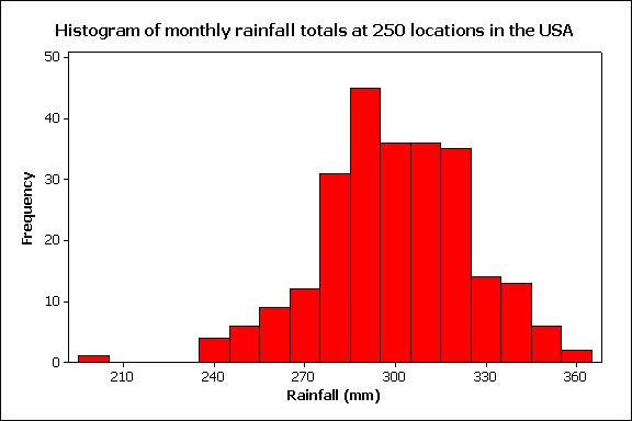
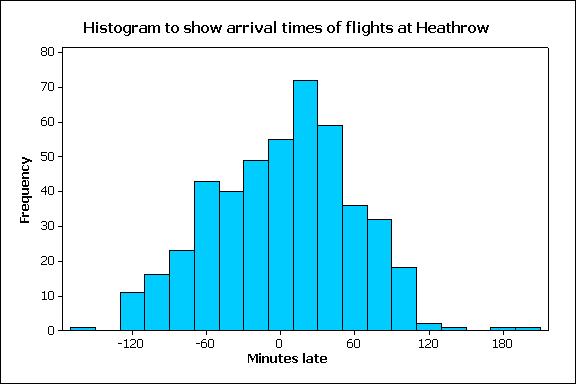
7 Announcements: Written assignment (mini project) You should be working on this now; worth 10% of the module; deadline for submission: 4pm, Thursday 13th December Hints: Graphs: when comparing two or more groups, use the same scales (e.g. percentage rel. freq. histograms or polygons, x-axes etc.)......and where appropriate overlay graphs on the same panel Produce appropriate graphical / numerical summaries... : Numerical one measure of average + one measure of spread per dataset; Graphical one or two at most per dataset Comments: Average? Where does the graph peak? Spread / dispersion? Outliers? Symmetric / asymmetric distribution? Normal distribution?
8 Announcements: Written assignment (mini project) You should be working on this now; worth 10% of the module; deadline for submission: 4pm, Thursday 13th December Hints: Graphs: when comparing two or more groups, use the same scales (e.g. percentage rel. freq. histograms or polygons, x-axes etc.)......and where appropriate overlay graphs on the same panel Produce appropriate graphical / numerical summaries... : Numerical one measure of average + one measure of spread per dataset; Graphical one or two at most per dataset Comments: Average? Where does the graph peak? Spread / dispersion? Outliers? Symmetric / asymmetric distribution? Normal distribution?
9 Announcements: Written assignment (mini project) Submission:
10 Announcements: Written assignment (mini project) Submission: Hard-copy, posted through the Stage 1 homework submission letterbox on the 3rd floor of the Herschel Building
11 Announcements: Written assignment (mini project) Submission: Hard-copy, posted through the Stage 1 homework submission letterbox on the 3rd floor of the Herschel Building Must have a personalised NESS cover sheet attached
12 Announcements: Written assignment (mini project) Submission: Hard-copy, posted through the Stage 1 homework submission letterbox on the 3rd floor of the Herschel Building Must have a personalised NESS cover sheet attached Personalised datasets for question 2!
13 Announcements: Written assignment (mini project) Submission: Hard-copy, posted through the Stage 1 homework submission letterbox on the 3rd floor of the Herschel Building Must have a personalised NESS cover sheet attached Personalised datasets for question 2! Marks for presentation: Type up solutions in WORD?
14 Announcements CBA3: Will go live at 00:01 this coming Saturday, 1st December in both practice and assessed modes
15 Announcements CBA3: Will go live at 00:01 this coming Saturday, 1st December in both practice and assessed modes Deadline: 23:59 Friday 14th December
16 Lecture 9 CONTINUOUS PROBABILITY MODELS
17 9. Continuous probability models We have seen how discrete random variables can be modelled by discrete probability distributions such as the binomial and Poisson distributions. We now consider how to model continuous random variables.
18 9. Continuous probability models A variable is discrete if it takes a countable number of values. For example, the number of blue cars that I count in a 5 minute period the number of heads observed when I flip a coin ten times Shoe sizes: 1,...,12, 13, 1, 2,... r = 0, 0.1, 0.2,...,0.9, 1.0
19 9. Continuous probability models A variable is discrete if it takes a countable number of values. For example, the number of blue cars that I count in a 5 minute period the number of heads observed when I flip a coin ten times Shoe sizes: 1,...,12, 13, 1, 2,... r = 0, 0.1, 0.2,...,0.9, 1.0 In contrast, the values which a continuous variable can take form a continuous scale, with no jumps. For example, Height Weight Temperature
20 An example Think about height. In practice, we might only record height to the nearest cm If we could measure height exactly we d find that everyone had a different height This is the essential difference between discrete and continuous variables If there are n people on the planet, the probability that someone s height is x would be 1 n As n gets bigger and bigger, this probability tends to zero!!

21 An example Consider taking a sample of values from the continuous random variable X.
22 An example As the sample size gets bigger, the interval widths get smaller the jagged profile of the histogram smooths out to become a curve When the sample size is infinitely large, this curve is known as the probability density function (pdf)
23 Features of the probability density function The key features of pdfs are: 1 the area under a pdf is one: P( < X < ) = 1 2 areas under the curve correspond to probabilities 3 P(X x) = P(X < x) since P(X = x) = 0.
24 9. Continuous probability models Over the next two weeks we will consider some particular probability distributions that are often used to describe continuous random variables.
25 9. Continuous probability models Over the next two weeks we will consider some particular probability distributions that are often used to describe continuous random variables. We start with the most important, most widely used statistical distribution of all time...
26 9. Continuous probability models Over the next two weeks we will consider some particular probability distributions that are often used to describe continuous random variables. We start with the most important, most widely used statistical distribution of all time......wait for it...
27 9. Continuous probability models The Normal Distribution
28 9.1 The Normal distribution The Normal distribution is without doubt the most widely-used statistical distribution in many practical applications:
29 9.1 The Normal distribution The Normal distribution is without doubt the most widely-used statistical distribution in many practical applications: Normality arises naturally in many physical, biological and social measurement situations
30 9.1 The Normal distribution The Normal distribution is without doubt the most widely-used statistical distribution in many practical applications: Normality arises naturally in many physical, biological and social measurement situations Normality is important in Statistical inference (see Semester 2 material)

 The normal distribution has many guises: Gaussian distribution Laplacean distribution bell")
31 9.1 The Normal distribution The Normal distribution is without doubt the most widely-used statistical distribution in many practical applications: Normality arises naturally in many physical, biological and social measurement situations Normality is important in Statistical inference (see Semester 2 material) The normal distribution has many guises: Gaussian distribution Laplacean distribution bell shaped curve

32 Some real life examples
33 9.1 The Normal distribution Recall the parameters of the binomial and Poisson distributions: The binomial distribution has two parameters, n and p the Poisson distribution has one parameter λ
34 9.1 The Normal distribution Recall the parameters of the binomial and Poisson distributions: The binomial distribution has two parameters, n and p the Poisson distribution has one parameter λ The Normal distribution has two parameters: the mean, µ, and the standard deviation, σ
35 9.1 The Normal distribution The probability density function (pdf) of the Normal distribution has a bell shaped profile: f(x) µ 4σ µ 2σ µ µ+2σ µ+4σ x
36 9.1 The Normal distribution We can think of the pdf as a smoothed percentage relative frequency histogram: the area under the curve is 1.
37 9.1 The Normal distribution We can think of the pdf as a smoothed percentage relative frequency histogram: the area under the curve is 1. The (rather nasty!) formula for this pdf is f(x) = { } 1 exp (x µ)2 2πσ 2 2σ 2. Unlike the binomial and Poisson distributions, there is no simple formula for calculating probabilities. Don t worry though, probabilities from the Normal distribution can be determined using statistical tables (see page 51) or statistical packages such asminitab.
38 Characteristics of the Normal distribution There are four important characteristics of the Normal distribution: 1 It is symmetrical about its mean, µ. 2 The mean, median and mode all coincide. 3 The area under the curve is equal to 1. 4 The curve extends in both directions to infinity ( ). On the next slide are plots of the pdf for Normal distributions with different values of µ and σ.
39
40 Notation If a random variable X has a Normal distribution with mean µ and variance σ 2, then we write ( X N µ,σ 2).
41 Notation If a random variable X has a Normal distribution with mean µ and variance σ 2, then we write ( X N µ,σ 2). For example, a random variable X which follows a Normal distribution with mean 10 and variance 25 is written as X N(10, 25) or ( X N 10, 5 2).
42 Notation If a random variable X has a Normal distribution with mean µ and variance σ 2, then we write ( X N µ,σ 2). For example, a random variable X which follows a Normal distribution with mean 10 and variance 25 is written as X N(10, 25) or ( X N 10, 5 2). It is important to note that the second parameter in this notation is the variance and not the standard deviation.
43 9.1.1 The standard Normal distribution The Standard Normal distribution has a mean of 0 and a variance of 1. A random variable with this standard Normal distribution is usually given the letter Z, and so we say Z N(0, 1).
44 9.1.1 The standard Normal distribution The Standard Normal distribution has a mean of 0 and a variance of 1. A random variable with this standard Normal distribution is usually given the letter Z, and so we say Z N(0, 1). If our random variable follows a standard Normal distribution, then we can obtain cumulative probabilities from statistical tables (see page 51 of the notes), which give less than or equal to probabilities.
45 Probability density function for Z PDF of the standard Normal distribution
46 Example 1 For example, if Z N(0, 1):
47 Example 1 For example, if Z N(0, 1): (a) The probability that Z is less than or equal to 1.46 is P(Z 1.46). Therefore we look for the probability in tables corresponding to z = 1.46: row labelled 1.4, column headed This gives P(Z 1.46) =
48 Example 1 For example, if Z N(0, 1): (a) The probability that Z is less than or equal to 1.46 is P(Z 1.46). Therefore we look for the probability in tables corresponding to z = 1.46: row labelled 1.4, column headed This gives P(Z 1.46) = (b) The probability that Z is less than or equal to 0.01 is P(Z 0.01). Therefore we look for the probability in tables corresponding to z = 0.01: row labelled 0.0, column headed This gives P(Z 0.01) =
49 Example 1 (c) The probability that Z is greater than 1.5 is P(Z > 1.5). Now our tables give less than probabilities, and here we want a greater than probability.
50 Example 1 (c) The probability that Z is greater than 1.5 is P(Z > 1.5). Now our tables give less than probabilities, and here we want a greater than probability.
51 Example 1 (c) The probability that Z is greater than 1.5 is P(Z > 1.5). Now our tables give less than probabilities, and here we want a greater than probability. So we find P(Z < 1.5) = and subtract this from 1 to give
52 Example 1 (d) What about the probability that Z lies between 1.2 and 1.5? It helps to think about this graphically.
53 Example 1 (d) What about the probability that Z lies between 1.2 and 1.5? It helps to think about this graphically. Doing so, gives: P( 1.2 < Z < 1.5)= P(Z < 1.5) P(Z 1.2) = =
54 Example 1 (d) What about the probability that Z lies between 1.2 and 1.5? It often helps to think about this graphically. Doing so, gives: P( 1.2 < Z < 1.5)= P(Z < 1.5) P(Z 1.2) = =
55 Example 1 (d) What about the probability that Z lies between 1.2 and 1.5? It often helps to think about this graphically.
56 Example 1 (d) What about the probability that Z lies between 1.2 and 1.5? It often helps to think about this graphically. Doing so, gives P( 1.2 < Z < 1.5) = P(Z < 1.5) P(Z 1.2) = =
57 Example 1 (e) P(Z < 1.5) = 1 P(Z > 1.5)
58 Example 1 (e) P(Z < 1.5) = 1 P(Z > 1.5) = From part (c)
59 Example 1 (e) P(Z < 1.5) = 1 P(Z > 1.5) = From part (c) =
60 9.1.2 Probabilities from any Normal distribution So how do we calculate probabilities for any Normal distribution, not just the standard Normal distribution (for which we have tables)? Idea: make the Normal distribution that we have look like the standard Normal distribution, and then we can just use the tables as before! But how? Use the slide squash technique!
61 9.1.2 Probabilities from any Normal distribution The formula which changes any Normal random variable X into the standard Normal random variable Z is given by where µ is the mean σ is the standard deviation Z = X µ, σ This can be translated into probability statements: ( P(X x) = P Z x µ ), σ which can be looked up in tables.
62 Example 2 If X N(10, 2 2 ), calculate P(X 8).
63 Example 2 If X N(10, 2 2 ), calculate P(X 8). Translate X into Z using the slide-squash rule: Z = X µ σ
64 Example 2 If X N(10, 2 2 ), calculate P(X 8). Translate X into Z using the slide-squash rule: Z = X µ σ =
65 Example 2 If X N(10, 2 2 ), calculate P(X 8). Translate X into Z using the slide-squash rule: Z = X µ σ = = 1.
66 Example 2 If X N(10, 2 2 ), calculate P(X 8). Translate X into Z using the slide-squash rule: Z = X µ σ = = 1. Then, from the table on page 51, P(Z 1) =
67 Example 3 Suppose X is the IQ of a randomly selected year old and that X follows a normal distribution with mean µ = 100 and standard deviation σ = 15. Thus, we have: ( X N 100, 15 2). Find the following probabilities. (a) (b) (c) (d) The probability that an year old has an IQ less than 110. The probability that an year old has an IQ greater than 110. The probability that an year old has an IQ greater than 125. The probability that an year old has an IQ between 95 and 115.
68 Example 3 Distribution of IQs
69 Example 3 Slide squash
70 Example 3 Slide squash
71 Example 3 Slide squash
72 Example 3 Slide squash
73 Example 3 Slide squash
74 Example 3 Slide squash
75 Example 3 Slide squash
76 Example 3 Slide squash
77 Example 3 Slide squash
78 Example 3 Slide squash
79 Example 3 Slide squash
80 Example 3 (a) P(X < 110) = P ( Z < X µ ) σ
81 Example 3 (a) P(X < 110) = P = P ( Z < X µ ) σ ( Z < ) 15
82 Example 3 (a) P(X < 110) = P = P ( Z < X µ ) σ ( Z < ) 15 = P(Z < 0.67)
83 Example 3 (a) P(X < 110) = P = P ( Z < X µ ) σ ( Z < ) 15 = P(Z < 0.67) =
84 Example 3 (b) P(X > 110) = 1 P(X < 110)
85 Example 3 (b) P(X > 110) = 1 P(X < 110) =
86 Example 3 (b) P(X > 110) = 1 P(X < 110) = =
87 Example 3 (c) P(X > 125) = 1 P(X < 125)
88 Example 3 (c) P(X > 125) = 1 P(X < 125) = 1 P ( Z < ) 15
89 Example 3 (c) P(X > 125) = 1 P(X < 125) = 1 P ( Z < ) 15 = 1 P(Z < 1.67)
90 Example 3 (c) P(X > 125) = 1 P(X < 125) = 1 P ( Z < ) 15 = 1 P(Z < 1.67) =
91 Example 3 (c) P(X > 125) = 1 P(X < 125) = 1 P ( Z < ) 15 = 1 P(Z < 1.67) = =
92 Example 3 (d) P(95 < X < 115) = P(X < 115) P(X < 95)
93 Example 3 (d) P(95 < X < 115) = P(X < 115) P(X < 95) = P ( Z < ) 15
94 Example 3 (d) P(95 < X < 115) = P(X < 115) P(X < 95) = P ( Z < ) ( P Z < ) 15 15
95 Example 3 (d) P(95 < X < 115) = P(X < 115) P(X < 95) = P ( Z < ) ( P Z < ) = P(Z < 1)
96 Example 3 (d) P(95 < X < 115) = P(X < 115) P(X < 95) = P ( Z < ) ( P Z < ) = P(Z < 1) P(Z < 0.33)
97 Example 3 (d) P(95 < X < 115) = P(X < 115) P(X < 95) = P ( Z < ) ( P Z < ) = P(Z < 1) P(Z < 0.33) =
98 Example 3 (d) P(95 < X < 115) = P(X < 115) P(X < 95) = P ( Z < ) ( P Z < ) = P(Z < 1) P(Z < 0.33) =
99 Example 3 (d) P(95 < X < 115) = P(X < 115) P(X < 95) = P ( Z < ) ( P Z < ) = P(Z < 1) P(Z < 0.33) = =
ECON 214 Elements of Statistics for Economists 2016/2017
 ECON 214 Elements of Statistics for Economists 2016/2017 Topic The Normal Distribution Lecturer: Dr. Bernardin Senadza, Dept. of Economics bsenadza@ug.edu.gh College of Education School of Continuing and
ECON 214 Elements of Statistics for Economists
 ECON 214 Elements of Statistics for Economists Session 7 The Normal Distribution Part 1 Lecturer: Dr. Bernardin Senadza, Dept. of Economics Contact Information: bsenadza@ug.edu.gh College of Education
MAS187/AEF258. University of Newcastle upon Tyne
 MAS187/AEF258 University of Newcastle upon Tyne 2005-6 Contents 1 Collecting and Presenting Data 5 1.1 Introduction...................................... 5 1.1.1 Examples...................................
Department of Quantitative Methods & Information Systems. Business Statistics. Chapter 6 Normal Probability Distribution QMIS 120. Dr.
 Department of Quantitative Methods & Information Systems Business Statistics Chapter 6 Normal Probability Distribution QMIS 120 Dr. Mohammad Zainal Chapter Goals After completing this chapter, you should
2011 Pearson Education, Inc
 Statistics for Business and Economics Chapter 4 Random Variables & Probability Distributions Content 1. Two Types of Random Variables 2. Probability Distributions for Discrete Random Variables 3. The Binomial
Chapter ! Bell Shaped
 Chapter 6 6-1 Business Statistics: A First Course 5 th Edition Chapter 7 Continuous Probability Distributions Learning Objectives In this chapter, you learn:! To compute probabilities from the normal distribution!
Data Analysis and Statistical Methods Statistics 651
 Data Analysis and Statistical Methods Statistics 651 http://www.stat.tamu.edu/~suhasini/teaching.html Suhasini Subba Rao The binomial: mean and variance Recall that the number of successes out of n, denoted
Topic 6 - Continuous Distributions I. Discrete RVs. Probability Density. Continuous RVs. Background Reading. Recall the discrete distributions
 Topic 6 - Continuous Distributions I Discrete RVs Recall the discrete distributions STAT 511 Professor Bruce Craig Binomial - X= number of successes (x =, 1,...,n) Geometric - X= number of trials (x =,...)
Class 12. Daniel B. Rowe, Ph.D. Department of Mathematics, Statistics, and Computer Science. Marquette University MATH 1700
 Class 12 Daniel B. Rowe, Ph.D. Department of Mathematics, Statistics, and Computer Science Copyright 2017 by D.B. Rowe 1 Agenda: Recap Chapter 6.1-6.2 Lecture Chapter 6.3-6.5 Problem Solving Session. 2
Statistical Methods in Practice STAT/MATH 3379
 Statistical Methods in Practice STAT/MATH 3379 Dr. A. B. W. Manage Associate Professor of Mathematics & Statistics Department of Mathematics & Statistics Sam Houston State University Overview 6.1 Discrete
Lecture 9. Probability Distributions. Outline. Outline
 Outline Lecture 9 Probability Distributions 6-1 Introduction 6- Probability Distributions 6-3 Mean, Variance, and Expectation 6-4 The Binomial Distribution Outline 7- Properties of the Normal Distribution
Math 227 Elementary Statistics. Bluman 5 th edition
 Math 227 Elementary Statistics Bluman 5 th edition CHAPTER 6 The Normal Distribution 2 Objectives Identify distributions as symmetrical or skewed. Identify the properties of the normal distribution. Find
Lecture 9. Probability Distributions
 Lecture 9 Probability Distributions Outline 6-1 Introduction 6-2 Probability Distributions 6-3 Mean, Variance, and Expectation 6-4 The Binomial Distribution Outline 7-2 Properties of the Normal Distribution
CS 237: Probability in Computing
 CS 237: Probability in Computing Wayne Snyder Computer Science Department Boston University Lecture 12: Continuous Distributions Uniform Distribution Normal Distribution (motivation) Discrete vs Continuous
Basic Procedure for Histograms
 Basic Procedure for Histograms 1. Compute the range of observations (min. & max. value) 2. Choose an initial # of classes (most likely based on the range of values, try and find a number of classes that
ME3620. Theory of Engineering Experimentation. Spring Chapter III. Random Variables and Probability Distributions.
 ME3620 Theory of Engineering Experimentation Chapter III. Random Variables and Probability Distributions Chapter III 1 3.2 Random Variables In an experiment, a measurement is usually denoted by a variable
MAS1403. Quantitative Methods for Business Management. Semester 1, Module leader: Dr. David Walshaw
 MAS1403 Quantitative Methods for Business Management Semester 1, 2018 2019 Module leader: Dr. David Walshaw Additional lecturers: Dr. James Waldren and Dr. Stuart Hall Announcements This week is a computer
The Normal Probability Distribution
 1 The Normal Probability Distribution Key Definitions Probability Density Function: An equation used to compute probabilities for continuous random variables where the output value is greater than zero
Introduction to Business Statistics QM 120 Chapter 6
 DEPARTMENT OF QUANTITATIVE METHODS & INFORMATION SYSTEMS Introduction to Business Statistics QM 120 Chapter 6 Spring 2008 Chapter 6: Continuous Probability Distribution 2 When a RV x is discrete, we can
Section 7.5 The Normal Distribution. Section 7.6 Application of the Normal Distribution
 Section 7.6 Application of the Normal Distribution A random variable that may take on infinitely many values is called a continuous random variable. A continuous probability distribution is defined by
STAT 201 Chapter 6. Distribution
 STAT 201 Chapter 6 Distribution 1 Random Variable We know variable Random Variable: a numerical measurement of the outcome of a random phenomena Capital letter refer to the random variable Lower case letters
Statistics 6 th Edition
 Statistics 6 th Edition Chapter 5 Discrete Probability Distributions Chap 5-1 Definitions Random Variables Random Variables Discrete Random Variable Continuous Random Variable Ch. 5 Ch. 6 Chap 5-2 Discrete
Week 1 Variables: Exploration, Familiarisation and Description. Descriptive Statistics.
 Week 1 Variables: Exploration, Familiarisation and Description. Descriptive Statistics. Convergent validity: the degree to which results/evidence from different tests/sources, converge on the same conclusion.
Some Characteristics of Data
 Some Characteristics of Data Not all data is the same, and depending on some characteristics of a particular dataset, there are some limitations as to what can and cannot be done with that data. Some key
Introduction to Statistics I
 Introduction to Statistics I Keio University, Faculty of Economics Continuous random variables Simon Clinet (Keio University) Intro to Stats November 1, 2018 1 / 18 Definition (Continuous random variable)
The normal distribution is a theoretical model derived mathematically and not empirically.
 Sociology 541 The Normal Distribution Probability and An Introduction to Inferential Statistics Normal Approximation The normal distribution is a theoretical model derived mathematically and not empirically.
Theoretical Foundations
 Theoretical Foundations Probabilities Monia Ranalli monia.ranalli@uniroma2.it Ranalli M. Theoretical Foundations - Probabilities 1 / 27 Objectives understand the probability basics quantify random phenomena
CH 5 Normal Probability Distributions Properties of the Normal Distribution
 Properties of the Normal Distribution Example A friend that is always late. Let X represent the amount of minutes that pass from the moment you are suppose to meet your friend until the moment your friend
Statistics for Business and Economics
 Statistics for Business and Economics Chapter 5 Continuous Random Variables and Probability Distributions Ch. 5-1 Probability Distributions Probability Distributions Ch. 4 Discrete Continuous Ch. 5 Probability
Statistics 511 Supplemental Materials
 Gaussian (or Normal) Random Variable In this section we introduce the Gaussian Random Variable, which is more commonly referred to as the Normal Random Variable. This is a random variable that has a bellshaped
Chapter 5. Continuous Random Variables and Probability Distributions. 5.1 Continuous Random Variables
 Chapter 5 Continuous Random Variables and Probability Distributions 5.1 Continuous Random Variables 1 2CHAPTER 5. CONTINUOUS RANDOM VARIABLES AND PROBABILITY DISTRIBUTIONS Probability Distributions Probability
Lecture Slides. Elementary Statistics Tenth Edition. by Mario F. Triola. and the Triola Statistics Series. Slide 1
 Lecture Slides Elementary Statistics Tenth Edition and the Triola Statistics Series by Mario F. Triola Slide 1 Chapter 6 Normal Probability Distributions 6-1 Overview 6-2 The Standard Normal Distribution
Business Statistics 41000: Probability 3
 Business Statistics 41000: Probability 3 Drew D. Creal University of Chicago, Booth School of Business February 7 and 8, 2014 1 Class information Drew D. Creal Email: dcreal@chicagobooth.edu Office: 404
CHAPTER 8 PROBABILITY DISTRIBUTIONS AND STATISTICS
 CHAPTER 8 PROBABILITY DISTRIBUTIONS AND STATISTICS 8.1 Distribution of Random Variables Random Variable Probability Distribution of Random Variables 8.2 Expected Value Mean Mean is the average value of
Class 11. Daniel B. Rowe, Ph.D. Department of Mathematics, Statistics, and Computer Science. Marquette University MATH 1700
 Class 11 Daniel B. Rowe, Ph.D. Department of Mathematics, Statistics, and Computer Science Copyright 2017 by D.B. Rowe 1 Agenda: Recap Chapter 5.3 continued Lecture 6.1-6.2 Go over Eam 2. 2 5: Probability
4: Probability. Notes: Range of possible probabilities: Probabilities can be no less than 0% and no more than 100% (of course).
.") 4: Probability What is probability? The probability of an event is its relative frequency (proportion) in the population. An event that happens half the time (such as a head showing up on the flip of a
4: Probability What is probability? The probability of an event is its relative frequency (proportion) in the population. An event that happens half the time (such as a head showing up on the flip of a
The Normal Distribution
 5.1 Introduction to Normal Distributions and the Standard Normal Distribution Section Learning objectives: 1. How to interpret graphs of normal probability distributions 2. How to find areas under the
Chapter 6. The Normal Probability Distributions
 Chapter 6 The Normal Probability Distributions 1 Chapter 6 Overview Introduction 6-1 Normal Probability Distributions 6-2 The Standard Normal Distribution 6-3 Applications of the Normal Distribution 6-5
ECO220Y Continuous Probability Distributions: Normal Readings: Chapter 9, section 9.10
 ECO220Y Continuous Probability Distributions: Normal Readings: Chapter 9, section 9.10 Fall 2011 Lecture 8 Part 2 (Fall 2011) Probability Distributions Lecture 8 Part 2 1 / 23 Normal Density Function f
Section Introduction to Normal Distributions
 Section 6.1-6.2 Introduction to Normal Distributions 2012 Pearson Education, Inc. All rights reserved. 1 of 105 Section 6.1-6.2 Objectives Interpret graphs of normal probability distributions Find areas
Class 16. Daniel B. Rowe, Ph.D. Department of Mathematics, Statistics, and Computer Science. Marquette University MATH 1700
 Class 16 Daniel B. Rowe, Ph.D. Department of Mathematics, Statistics, and Computer Science Copyright 013 by D.B. Rowe 1 Agenda: Recap Chapter 7. - 7.3 Lecture Chapter 8.1-8. Review Chapter 6. Problem Solving
Example - Let X be the number of boys in a 4 child family. Find the probability distribution table:
 Chapter7 Probability Distributions and Statistics Distributions of Random Variables tthe value of the result of the probability experiment is a RANDOM VARIABLE. Example - Let X be the number of boys in
Homework: Due Wed, Nov 3 rd Chapter 8, # 48a, 55c and 56 (count as 1), 67a
, 67a") Homework: Due Wed, Nov 3 rd Chapter 8, # 48a, 55c and 56 (count as 1), 67a Announcements: There are some office hour changes for Nov 5, 8, 9 on website Week 5 quiz begins after class today and ends at
Homework: Due Wed, Nov 3 rd Chapter 8, # 48a, 55c and 56 (count as 1), 67a Announcements: There are some office hour changes for Nov 5, 8, 9 on website Week 5 quiz begins after class today and ends at
A LEVEL MATHEMATICS ANSWERS AND MARKSCHEMES SUMMARY STATISTICS AND DIAGRAMS. 1. a) 45 B1 [1] b) 7 th value 37 M1 A1 [2]
![A LEVEL MATHEMATICS ANSWERS AND MARKSCHEMES SUMMARY STATISTICS AND DIAGRAMS. 1. a) 45 B1 [1] b) 7 th value 37 M1 A1 [2]](/thumbs/81/83043398.jpg "A LEVEL MATHEMATICS ANSWERS AND MARKSCHEMES SUMMARY STATISTICS AND DIAGRAMS. 1. a) 45 B1 [1] b) 7 th value 37 M1 A1 [2]") 1. a) 45 [1] b) 7 th value 37 [] n c) LQ : 4 = 3.5 4 th value so LQ = 5 3 n UQ : 4 = 9.75 10 th value so UQ = 45 IQR = 0 f.t. d) Median is closer to upper quartile Hence negative skew [] Page 1 . a) Orders
1. a) 45 [1] b) 7 th value 37 [] n c) LQ : 4 = 3.5 4 th value so LQ = 5 3 n UQ : 4 = 9.75 10 th value so UQ = 45 IQR = 0 f.t. d) Median is closer to upper quartile Hence negative skew [] Page 1 . a) Orders
Chapter 4 Continuous Random Variables and Probability Distributions
 Chapter 4 Continuous Random Variables and Probability Distributions Part 2: More on Continuous Random Variables Section 4.5 Continuous Uniform Distribution Section 4.6 Normal Distribution 1 / 27 Continuous
Probability. An intro for calculus students P= Figure 1: A normal integral
 Probability An intro for calculus students.8.6.4.2 P=.87 2 3 4 Figure : A normal integral Suppose we flip a coin 2 times; what is the probability that we get more than 2 heads? Suppose we roll a six-sided
MAKING SENSE OF DATA Essentials series
 MAKING SENSE OF DATA Essentials series THE NORMAL DISTRIBUTION Copyright by City of Bradford MDC Prerequisites Descriptive statistics Charts and graphs The normal distribution Surveys and sampling Correlation
A.REPRESENTATION OF DATA
 A.REPRESENTATION OF DATA (a) GRAPHS : PART I Q: Why do we need a graph paper? Ans: You need graph paper to draw: (i) Histogram (ii) Cumulative Frequency Curve (iii) Frequency Polygon (iv) Box-and-Whisker
Chapter 4 Random Variables & Probability. Chapter 4.5, 6, 8 Probability Distributions for Continuous Random Variables
 Chapter 4.5, 6, 8 Probability for Continuous Random Variables Discrete vs. continuous random variables Examples of continuous distributions o Uniform o Exponential o Normal Recall: A random variable =
Expected Value of a Random Variable
 Knowledge Article: Probability and Statistics Expected Value of a Random Variable Expected Value of a Discrete Random Variable You're familiar with a simple mean, or average, of a set. The mean value of
Chapter 4 Continuous Random Variables and Probability Distributions
 Chapter 4 Continuous Random Variables and Probability Distributions Part 2: More on Continuous Random Variables Section 4.5 Continuous Uniform Distribution Section 4.6 Normal Distribution 1 / 28 One more
Chapter 4 Probability and Probability Distributions. Sections
 Chapter 4 Probabilit and Probabilit Distributions Sections 4.6-4.10 Sec 4.6 - Variables Variable: takes on different values (or attributes) Random variable: cannot be predicted with certaint Random Variables
Chapter 6 Continuous Probability Distributions. Learning objectives
 Chapter 6 Continuous s Slide 1 Learning objectives 1. Understand continuous probability distributions 2. Understand Uniform distribution 3. Understand Normal distribution 3.1. Understand Standard normal
ECON 214 Elements of Statistics for Economists 2016/2017
 ECON 214 Elements of Statistics for Economists 2016/2017 Topic Probability Distributions: Binomial and Poisson Distributions Lecturer: Dr. Bernardin Senadza, Dept. of Economics bsenadza@ug.edu.gh College
Statistics (This summary is for chapters 17, 28, 29 and section G of chapter 19)
") Statistics (This summary is for chapters 17, 28, 29 and section G of chapter 19) Mean, Median, Mode Mode: most common value Median: middle value (when the values are in order) Mean = total how many = x
Statistics (This summary is for chapters 17, 28, 29 and section G of chapter 19) Mean, Median, Mode Mode: most common value Median: middle value (when the values are in order) Mean = total how many = x
Statistics, Measures of Central Tendency I
 Statistics, Measures of Central Tendency I We are considering a random variable X with a probability distribution which has some parameters. We want to get an idea what these parameters are. We perfom
23.1 Probability Distributions
 3.1 Probability Distributions Essential Question: What is a probability distribution for a discrete random variable, and how can it be displayed? Explore Using Simulation to Obtain an Empirical Probability
Describing Uncertain Variables
 Describing Uncertain Variables L7 Uncertainty in Variables Uncertainty in concepts and models Uncertainty in variables Lack of precision Lack of knowledge Variability in space/time Describing Uncertainty
Lecture 12. Some Useful Continuous Distributions. The most important continuous probability distribution in entire field of statistics.
 ENM 207 Lecture 12 Some Useful Continuous Distributions Normal Distribution The most important continuous probability distribution in entire field of statistics. Its graph, called the normal curve, is
MAS3904/MAS8904 Stochastic Financial Modelling
 MAS3904/MAS8904 Stochastic Financial Modelling Dr Andrew (Andy) Golightly a.golightly@ncl.ac.uk Semester 1, 2018/19 Administrative Arrangements Lectures on Tuesdays at 14:00 (PERCY G13) and Thursdays at
STAT Chapter 5: Continuous Distributions. Probability distributions are used a bit differently for continuous r.v. s than for discrete r.v. s.
 STAT 515 -- Chapter 5: Continuous Distributions Probability distributions are used a bit differently for continuous r.v. s than for discrete r.v. s. Continuous distributions typically are represented by
Math 14 Lecture Notes Ch The Normal Approximation to the Binomial Distribution. P (X ) = nc X p X q n X =
 = nc X p X q n X =") 6.4 The Normal Approximation to the Binomial Distribution Recall from section 6.4 that g A binomial experiment is a experiment that satisfies the following four requirements: 1. Each trial can have only
6.4 The Normal Approximation to the Binomial Distribution Recall from section 6.4 that g A binomial experiment is a experiment that satisfies the following four requirements: 1. Each trial can have only
A continuous random variable is one that can theoretically take on any value on some line interval. We use f ( x)
") Section 6-2 I. Continuous Probability Distributions A continuous random variable is one that can theoretically take on any value on some line interval. We use f ( x) to represent a probability density
Section 6-2 I. Continuous Probability Distributions A continuous random variable is one that can theoretically take on any value on some line interval. We use f ( x) to represent a probability density
Fundamentals of Statistics
 CHAPTER 4 Fundamentals of Statistics Expected Outcomes Know the difference between a variable and an attribute. Perform mathematical calculations to the correct number of significant figures. Construct
Business Statistics 41000: Probability 4
 Business Statistics 41000: Probability 4 Drew D. Creal University of Chicago, Booth School of Business February 14 and 15, 2014 1 Class information Drew D. Creal Email: dcreal@chicagobooth.edu Office:
Uniform Probability Distribution. Continuous Random Variables &
 Continuous Random Variables & What is a Random Variable? It is a quantity whose values are real numbers and are determined by the number of desired outcomes of an experiment. Is there any special Random
Chapter 7 1. Random Variables
 Chapter 7 1 Random Variables random variable numerical variable whose value depends on the outcome of a chance experiment - discrete if its possible values are isolated points on a number line - continuous
MA 1125 Lecture 18 - Normal Approximations to Binomial Distributions. Objectives: Compute probabilities for a binomial as a normal distribution.
 MA 25 Lecture 8 - Normal Approximations to Binomial Distributions Friday, October 3, 207 Objectives: Compute probabilities for a binomial as a normal distribution.. Normal Approximations to the Binomial
Examples: Random Variables. Discrete and Continuous Random Variables. Probability Distributions
 Random Variables Examples: Random variable a variable (typically represented by x) that takes a numerical value by chance. Number of boys in a randomly selected family with three children. Possible values:
Continuous Probability Distributions & Normal Distribution
 Mathematical Methods Units 3/4 Student Learning Plan Continuous Probability Distributions & Normal Distribution 7 lessons Notes: Students need practice in recognising whether a problem involves a discrete
Example - Let X be the number of boys in a 4 child family. Find the probability distribution table:
 Chapter8 Probability Distributions and Statistics Section 8.1 Distributions of Random Variables tthe value of the result of the probability experiment is a RANDOM VARIABLE. Example - Let X be the number
STAT Chapter 5: Continuous Distributions. Probability distributions are used a bit differently for continuous r.v. s than for discrete r.v. s.
 STAT 515 -- Chapter 5: Continuous Distributions Probability distributions are used a bit differently for continuous r.v. s than for discrete r.v. s. Continuous distributions typically are represented by
NORMAL RANDOM VARIABLES (Normal or gaussian distribution)
") NORMAL RANDOM VARIABLES (Normal or gaussian distribution) Many variables, as pregnancy lengths, foot sizes etc.. exhibit a normal distribution. The shape of the distribution is a symmetric bell shape.
NORMAL RANDOM VARIABLES (Normal or gaussian distribution) Many variables, as pregnancy lengths, foot sizes etc.. exhibit a normal distribution. The shape of the distribution is a symmetric bell shape.
value BE.104 Spring Biostatistics: Distribution and the Mean J. L. Sherley
 BE.104 Spring Biostatistics: Distribution and the Mean J. L. Sherley Outline: 1) Review of Variation & Error 2) Binomial Distributions 3) The Normal Distribution 4) Defining the Mean of a population Goals:
BIOL The Normal Distribution and the Central Limit Theorem
 BIOL 300 - The Normal Distribution and the Central Limit Theorem In the first week of the course, we introduced a few measures of center and spread, and discussed how the mean and standard deviation are
Part V - Chance Variability
 Part V - Chance Variability Dr. Joseph Brennan Math 148, BU Dr. Joseph Brennan (Math 148, BU) Part V - Chance Variability 1 / 78 Law of Averages In Chapter 13 we discussed the Kerrich coin-tossing experiment.
Homework: Due Wed, Feb 20 th. Chapter 8, # 60a + 62a (count together as 1), 74, 82
, 74, 82") Announcements: Week 5 quiz begins at 4pm today and ends at 3pm on Wed If you take more than 20 minutes to complete your quiz, you will only receive partial credit. (It doesn t cut you off.) Today: Sections
Announcements: Week 5 quiz begins at 4pm today and ends at 3pm on Wed If you take more than 20 minutes to complete your quiz, you will only receive partial credit. (It doesn t cut you off.) Today: Sections
UQ, STAT2201, 2017, Lectures 3 and 4 Unit 3 Probability Distributions.
 UQ, STAT2201, 2017, Lectures 3 and 4 Unit 3 Probability Distributions. Random Variables 2 A random variable X is a numerical (integer, real, complex, vector etc.) summary of the outcome of the random experiment.
Lecture 2 Describing Data
 Lecture 2 Describing Data Thais Paiva STA 111 - Summer 2013 Term II July 2, 2013 Lecture Plan 1 Types of data 2 Describing the data with plots 3 Summary statistics for central tendency and spread 4 Histograms
The topics in this section are related and necessary topics for both course objectives.
 2.5 Probability Distributions The topics in this section are related and necessary topics for both course objectives. A probability distribution indicates how the probabilities are distributed for outcomes
Lecture 6: Chapter 6
 Lecture 6: Chapter 6 C C Moxley UAB Mathematics 3 October 16 6.1 Continuous Probability Distributions Last week, we discussed the binomial probability distribution, which was discrete. 6.1 Continuous Probability
Chapter 4. The Normal Distribution
 Chapter 4 The Normal Distribution 1 Chapter 4 Overview Introduction 4-1 Normal Distributions 4-2 Applications of the Normal Distribution 4-3 The Central Limit Theorem 4-4 The Normal Approximation to the
AP Statistics Chapter 6 - Random Variables
 AP Statistics Chapter 6 - Random 6.1 Discrete and Continuous Random Objective: Recognize and define discrete random variables, and construct a probability distribution table and a probability histogram
The Normal Distribution
 Stat 6 Introduction to Business Statistics I Spring 009 Professor: Dr. Petrutza Caragea Section A Tuesdays and Thursdays 9:300:50 a.m. Chapter, Section.3 The Normal Distribution Density Curves So far we
Lecture 1: Review and Exploratory Data Analysis (EDA)
") Lecture 1: Review and Exploratory Data Analysis (EDA) Ani Manichaikul amanicha@jhsph.edu 16 April 2007 1 / 40 Course Information I Office hours For questions and help When? I ll announce this tomorrow
Lecture 1: Review and Exploratory Data Analysis (EDA) Ani Manichaikul amanicha@jhsph.edu 16 April 2007 1 / 40 Course Information I Office hours For questions and help When? I ll announce this tomorrow
Problems from 9th edition of Probability and Statistical Inference by Hogg, Tanis and Zimmerman:
 Math 224 Fall 207 Homework 5 Drew Armstrong Problems from 9th edition of Probability and Statistical Inference by Hogg, Tanis and Zimmerman: Section 3., Exercises 3, 0. Section 3.3, Exercises 2, 3, 0,.
AMS 7 Sampling Distributions, Central limit theorem, Confidence Intervals Lecture 4
 AMS 7 Sampling Distributions, Central limit theorem, Confidence Intervals Lecture 4 Department of Applied Mathematics and Statistics, University of California, Santa Cruz Summer 2014 1 / 26 Sampling Distributions!!!!!!
Chapter 4 Probability Distributions
 Slide 1 Chapter 4 Probability Distributions Slide 2 4-1 Overview 4-2 Random Variables 4-3 Binomial Probability Distributions 4-4 Mean, Variance, and Standard Deviation for the Binomial Distribution 4-5
MATH 104 CHAPTER 5 page 1 NORMAL DISTRIBUTION
 MATH 104 CHAPTER 5 page 1 NORMAL DISTRIBUTION We have examined discrete random variables, those random variables for which we can list the possible values. We will now look at continuous random variables.
What was in the last lecture?
 What was in the last lecture? Normal distribution A continuous rv with bell-shaped density curve The pdf is given by f(x) = 1 2πσ e (x µ)2 2σ 2, < x < If X N(µ, σ 2 ), E(X) = µ and V (X) = σ 2 Standard
Statistics for Business and Economics: Random Variables:Continuous
 Statistics for Business and Economics: Random Variables:Continuous STT 315: Section 107 Acknowledgement: I d like to thank Dr. Ashoke Sinha for allowing me to use and edit the slides. Murray Bourne (interactive
4.3 Normal distribution
 43 Normal distribution Prof Tesler Math 186 Winter 216 Prof Tesler 43 Normal distribution Math 186 / Winter 216 1 / 4 Normal distribution aka Bell curve and Gaussian distribution The normal distribution
MATH 264 Problem Homework I
 MATH Problem Homework I Due to December 9, 00@:0 PROBLEMS & SOLUTIONS. A student answers a multiple-choice examination question that offers four possible answers. Suppose that the probability that the
AMS7: WEEK 4. CLASS 3
 AMS7: WEEK 4. CLASS 3 Sampling distributions and estimators. Central Limit Theorem Normal Approximation to the Binomial Distribution Friday April 24th, 2015 Sampling distributions and estimators REMEMBER:
Commonly Used Distributions
 Chapter 4: Commonly Used Distributions 1 Introduction Statistical inference involves drawing a sample from a population and analyzing the sample data to learn about the population. We often have some knowledge
Chapter 7 Sampling Distributions and Point Estimation of Parameters
 Chapter 7 Sampling Distributions and Point Estimation of Parameters Part 1: Sampling Distributions, the Central Limit Theorem, Point Estimation & Estimators Sections 7-1 to 7-2 1 / 25 Statistical Inferences
HUDM4122 Probability and Statistical Inference. March 4, 2015
 HUDM4122 Probability and Statistical Inference March 4, 2015 First things first The Exam Due to Monday s class cancellation Today s lecture on the Normal Distribution will not be covered on the Midterm
STAT:2010 Statistical Methods and Computing. Using density curves to describe the distribution of values of a quantitative
 STAT:10 Statistical Methods and Computing Normal Distributions Lecture 4 Feb. 6, 17 Kate Cowles 374 SH, 335-0727 kate-cowles@uiowa.edu 1 2 Using density curves to describe the distribution of values of
Lecture 2. Probability Distributions Theophanis Tsandilas
 Lecture 2 Probability Distributions Theophanis Tsandilas Comment on measures of dispersion Why do common measures of dispersion (variance and standard deviation) use sums of squares: nx (x i ˆµ) 2 i=1
2. The sum of all the probabilities in the sample space must add up to 1
 Continuous Random Variables and Continuous Probability Distributions Continuous Random Variable: A variable X that can take values on an interval; key feature remember is that the values of the variable