Investigating the gender wage gap

Transcription

1 Mälardalen University Västerås, School of Sustainable Development of Society and Technology (HST) Bachelor Thesis in Economics Tutor: Johan Lindén Investigating the gender wage gap An econometric study on the Swedish Labor Market Per Jaldesjö,

2 Abstract Date: Level: Bachelor Thesis in Economics, 15 ECTS credits Author: Jaldesjö, Per Title: Investigating the gender wage gap An econometric study on the Swedish labor market Tutor: Johan Lindén, School of Sustainable Development of Society and Technology Problem: Purpose: Method: During the 20 th century the participation rate of women in the Swedish labor market increased more than in many other OECD-countries. The women-to-men wage ratio showed the same pattern until the 80 s when the pace slowed down. A consolidation of the inequalities has been the trend since. The primary aim of this thesis is to answer if inequalities in the parental leave are an important explanatory variable to the wage gap existing from Further employing sector is examined seeking to explain more of the wage inequalities. The model I have used is the Mincer earnings function modified for absence from work due to parental leave. Required data are collected and treated with statistical techniques. Based on this data OLS regression analysis is performed. Result and conclusion : The estimates indicate that the gender wage gap is caused by the inequalities in the withdrawal of the parental leave to the extent of 2.8%. The underrepresentation of women in the private sector is found to be more affecting but is also more likely to be biased. The return to schooling is found positive and similar for both genders. Likewise the return to OTJ is found positive, initially higher for men and after 23 years of accumulation somewhat higher for women. Mainly a higher relative educational level and increasing participation in the private sector is believed to explain the decrease of the wage gap. i

3 Table of contents 1. Introduction Litterature Aim Limitations Methodology Theoretical framework Compensating wage differentials Human capital theory The schooling model OTJ The Mincer earnings profile Econometrics The variables with data Wage Schooling Potential OTJ Sector OLS Multicollinearity Omitted variable Regression models Expectations Estimates Estimates of Models 1a-e Estimates of Models 2a-e Estimates of Models 1f-g and Models 2f-g Summary and conclusion References Literature Other sources Statistics Appendix Complete regression results from Table Complete regression results from Table Complete regression results from Table Supplement...40 Supplement 1 - Employed by sector ii

4 List of figures, diagrams and tables Figure 1 Indifference curves relating the wage and the probability of injury...6 Figure 2 Determining the market compensating differential...7 Figure 3 Potential areas of lifetime income...9 Diagram 1 Real wage gap year olds Diagram 2 Real wage gap year olds Diagram 3 Percentage of take-up of parental days by sex Diagram 4 Average wage by sector for men Diagram 5 Average wage by sector for women Table 1 Index of schooling duration Table 2 Average years of schooling Table 3 Expectations Table 4 Regression results for men with sector as changing variable Table 5 Regression results for women with sector as changing variable Table 6 Regression results without sector and with private sector iii

5 1. Introduction The changes on the labor markets over the last century have been progressive and releasing. The labor force participation rate of women has increased worldwide and in many countries, including the OECD members, the participation rate is nowadays close to those of men. Despite a slightly decline in recent years Sweden is, together with its Scandinavian neighbours Iceland and Norway, a top OECD country within the subject with a women labor force participation rate of 61% compared to 68% of the men (World Bank, 2012). Ever since the entrance there has on average been a wage gap between the genders. Sweden has stand out in international comparisons over time by having a relatively equal pay among the genders (Waldfogel, 1998). This was a result of decades of strong efforts from the Swedish government. Among others the legislation of equal pay for equal work and the establishment of universal childcare (Meyersson, Petersen & Snartland 2001). However this does not mean that the wages has in fact been equal. For example the women-to-men wage ratio was striking 58% in the Swedish manufacturing industry one century ago. Eighty years later the ratio had reached 89%. (Svensson, 1995). This trend has characterized the labor market as a whole but during the past two decades the pace of the tightening has been reduced remarkably. Despite more recent attempts of the government to abolish the gender imbalances on the labor market they have still not succeeded. High segregation within sectors and occupations together with an overrepresentation of women working part-time is besides the gender pay gap two big challenges for the government today. 1.1 Litterature A lot of research and reports made by academics and public authorities have been written in order to explain the gender wage gaps from all continents. I have looked at studies made on data from various decades from both Sweden and the US. To start in chronological order professor Lars Svensson (1995) investigated the reduction of the wage gap in blue collar jobs between Sweden Svensson stresses the importance of not taking the decreasing wage gap for granted. He shows how almost the whole reduction has taken place in only 27 years split into three periods of time. This occurred in a century when women labor supply increased steadily. This means that sometimes the increased labor supply outweighed the effect of the increased labor demand. 1

6 The greatest compression took place in the 60 s and 70 s. The solidaristic wage policy pushed through by Swedish confederation of Trade Unions (LO) is alleged to be a contributing factor together with an extension of public childcare and technological change in home production. The two latter factors were time saving and made it possible for more women to participate on the labor market (Nyberg, 1989). At the same year Morgan and Petersen (1995) made a study on the American labor market The study was inspecting both blue collar and clerical workers. One of their main results was pointing out job segregation as being the most important factor in both the categories. They also conclude that a substantial part of the wage gap cannot be explained by looking at schooling. More recent studies and reports of the Swedish labor market shows that the gender wage gap has not decreased in as in the prior decades (SCB 2002, 2010a, MI 2011). Occupations with the highest monthly wage also have the largest spread, the inequalities in salary are higher for men and the public sector has lower wage gaps than the private are their common results. SCB uses standard weighting and MI both standard weighting and regressions analysis 1. The variables chosen differ in number but age and educational level is the base used in all. The most recent study made by the National Mediation Office (MI) has three additional variables sector, occupation and level of employment. They found an unexplained wage gap of 5.4% which corresponds to about 38% of the total wage gap. Going back to the American labor market Waldfogel (1997) researched the effect of women being out of the labor market during parental leave. She found a direct wage lowering effect for mothers relative non-mothers, worse for mothers with more than one child. She conclude that after correcting for the difference in lost experience there was still a gap unexplained. Possible explanations she states may be discrimination or occupational downgrading. Budig and England (2001) did a similar study on more recent data influenced by Waldfogel. Their conclusion was that mothers are worse off than non-mothers with a wage penalty of 7%. The lost working experience during the maternity leave, causing lower productivity than otherwise, is estimated to explain one-third of the penalty. 1 (MI) reports that regression analysis is employed to deepen the analysis of the wage gap. Their regression analysis leaved an unexplained wage gap of 5.4% while the standard weighting method leaved 5.9% unexplained. (The actual wage gap of the period studied were 14.3%). 2

7 The aim of this thesis is chosen after inspiration from the study made by Budig and England together with the fact that I have not found any equivalent research on the gender wage gap 2 in the Swedish labor market. Since the parental leave in Sweden is more extended than in the United States the reducing effect on wage might be larger and inequalities be more decisive. 1.2 Aim This thesis will investigate the gender wage gap on the Swedish labor market between 1992 and The aim is to answer if inequalities in the take-up of the parental leave are an important contributor to the gender wage gap 3. What actually is investigated is approximately how big the loss of on-the-job training cost the mothers. I will also examine employing sector as an additional highly believed contributing factor. 1.3 Limitations Because of the time constraint some wage determining variables will be excluded from the regression model which is very likely to have effect. Occupation is probably the most important omitted variable. Hopefully it will not cause any severe bias but it will certainly leave a part of the wage gap unexplained. The study is made on panel data of different cohorts instead of individual data that often is used by researchers. This leads to a need for generalizations by using averages of fertility rates and sick leave rates. To calculate the parental leave a couple of simplifying assumptions are made: (1) workers in a certain age group are assumed to have the same fertility rate as the whole population of the same age, (2) teenage parents are assumed to not lose any potential on-the-job training just educational time, (3) fathers are assumed to be three years older than the mothers 4, (4) all households use the paid parental leave to its limit. The first assumption will cause a small underestimation of the parental leave, the second to a difference between the real on-the-job training and potential, the third to a little overestimation of the parental leave of young fathers and the opposite for the two oldest 2 Note the difference between the family wage gap which is the difference between mothers and non-mothers and the gender wage comparing all women and all men. 3 When the gender wage gap is mentioned I refer to the difference in wage between the 50th percentile of the genders, e.g. the median wage. The median is preferred to the average because of interpretational reasons. By using the median wage we know that we are inspecting the wage gap between the women and men who is paid less than half of the workers with the same sex and higher paid than the other half. 4 For motivation see Chapter 3.1 3

8 cohorts and the fourth to a little overestimation of the total-take up in more recent years due to the design of the parental leave 5. The data of employing sector during is less specific than the other years studied having only three cohorts. Two of these cohorts do not fit the rest of the data and are split into four cohorts with the same proportions as in the prior period. The data from the first part of the parental leave is not reported in specific numbers and are therefore approximated. Because of many made simplifications and possible data problems the results should not be seen as the definite answer rather an indication of the importance of the explanatory variables. 1.4 Methodology The theoretical part of this paper contains a number of models that examine central facts about the lead actors on the labor market, the employers and the workers. The model of compensating wage differentials shows how differences in preferences among workers result in the division of workers. Afterwards we take a close look at human capital accumulation. The schooling model show how long the optimal educational time is for a specific worker and the on-the-job training section contains facts of post-school human capital investments. Together with the model of human capital acquisition and the age earnings profile all these models are summing up into The Mincer earnings function which will be my tool for the empirical research. In the empirical part of the thesis I modify the Mincer earnings function a little bit to take the parental and sick leave of the genders into account with the econometric technique - Ordinary Least Square method (OLS). The OLS is used to make estimations about the wage determinants. The mentioned study made by Budig and England have encourage me to modifying the model used in the recent Swedish studies taking away age as an explanatory variable and substitute it with potential OTJ. As inputs in the regression data over wages, fertility rates, educational level and employing sector is collected from the Statistics Sweden (SCB) and data on sick leave has been taken from The Swedish Social Insurance Agency (FK). The data is managed to fit into the regression and the age-groups that are studied. After a detailed description of the empirical technique the regressions are executed. The resulting coefficients of the explanatory variables employed will be carefully treated and used in order to test to how much of the wage differentials, if anything, remains when correcting for inequalities in the independent variables. 5 For motivation see Chapter 3.1 4

9 2. Theoretical framework To investigate the gender wage gap with good understanding we first need to answer a question that have been asked for centuries: why do some people earn more than others? This part of the thesis will present a framework of wage determinants building the foundation of economic theory that the empirical research will rely on. 2.1 Compensating wage differentials First of all we can establish that all occupations are not equal. We have to consider all advantages and all disadvantages between them. According to Adam Smith (1772/2007), also known as the father of economics, there are five strongly influential circumstances that we should keep in mind. I find all these observations just as applicable to the labour market today as when it was written. First of all is how pleasant or unpleasant the activity is in itself. If employees prefer to work in big clean offices in the city instead of small filthy garages on the countryside they will tolerate a lower wage to get it. Secondly how easy and cheap or hard and costly it is to learn how to do the activity. If university studies would not repay the investment costs in a reasonable time fewer students would apply. For the third how constant or temporary the activities are. Staffing industry workers should for this cause get a wage premium compared to permanent employees. For the fourth how big responsibility has to be given to the practiser. CEO s doubtless have bigger responsibility than secretaries. And finally how big the risk of failure or forecast of success is. In the private sector companies have to be profitable to survive while the government in the role of lawmaker have the privilege to increase the revenues by tax raise, reducing the risk. All of Smith s five observations are examples of compensating wage differentials. Besides occupations being different workers also differ in their ability and preferences. We will examine the latter by using a very simplified version of the labor market made by Borjas (2010). Imagine a labor market consisting of only two types of jobs, safe and risky. Safe jobs have a probability of injury of 0 and risky jobs have the maximum number 1. The workers care about what type of job they have and how high their wages are. Therefore the utility function of the workers is: U = f (w, risk of injury). We assume that all workers are utility maximizers and that wage is a good and that all workers are risk averters thinking of the risk of injury as a bad e.g. consumption gives disutility. In a starting position where a worker are having a save job with the wage = w 0 she receives a utility of U 0, see figure 1. 5

10 Figure 1 We assume upward sloping convex indifference curves. The economic interpretation is that persuasion will be more and more expensive as riskier the job gets. The only chance of making this worker indifferent between the safe and risky job is to offer a compensating wage differential equal to Δ ŵ 1 so that the wage of the risky job = ŵ 1. This gives Δ ŵ 1 = ŵ 1 w 0. This sum is defined as the reservation price and can be seen as the answer to the question: How big wage raise must the worker is offered to work on job that she never would prefer with her initial wage w 1. Workers always differ in their preferences. If a worker is a extremely risk averter the bribe to make him work in a risky environment would be huge, while a worker who have preferences close to a risk neutral would accept a small bribe e.g. a small reservation price. Figure 2 illustrates the equilibrium of the labor market including the compensation for risk. The vertical axis measures the size of the compensation and the horizontal axis the number of workers in risky jobs. As the supply curve shows more and more workers are willing to work in a risky job when the compensation (w 1 -w 0 ) increases. The intercept is equal to the wage compensation as the least risk averting person would like to have to accept the risky job offer. 6

11 Figure 2 The employing company decides whether to offer a safe or risky environment depending on what is more profitable. If we assume that E* workers will be employed no matter of the level of risk we get the company s production function we get q 0 = α 0 E* where α 0 is the marginal product of labor in the safe environment. The price of output equals p dollars so the value of the marginal product of labor is p x α 0. If we then name MP of labor in risky jobs α 1 the VMP of labor on this job will be p x α 1. How does this two VMP s differ? It is easy to understand that providing safe working conditions does not come for free so α 1 > α 0. This implies that VMP will be higher on risky jobs therefore the revenues will be greater. The downside for these firms is that the workers want higher wage in return so the costs will also be higher in comparison with the safe-job offering firms. The profit functions being:. The employing company now choose the most profitable alternative. The dollar gain of switching from a safe to a risky environment can be defined as θ = pα 1 - pα 0. Therefore the company should choose to offer a safe environment if w 1 -w 0 > θ and conversely a risky environment if w 1 -w 0 < θ. We find the demand curve of risky firms by sum up the entire workers reservation price. Here the intercept is and as the compensation gets lower more firms find it profitable to offer risky jobs. We find the equilibrium where the demand curve equals our derived supply, which is illustrated by point P in figure 2. Here the compensating wage differential is and the number of workers E*. If this differential should be higher too many workers would want to be employed, as a response to the employer s too generous 7

12 offer. If the compensating wage differential would be less than would offer their services. too few workers 2.2 Human capital theory Besides preferences, workers, as mentioned, differ in other areas as well. An example is the variety of their investments. The investment in people or in human capital is not as noticeable as a company investing in a new plant or in the latest technology. However, in many western countries the investment in human capital have over the last century risen faster than for other production inputs such as land or physical capital and has perhaps become the main contributor to economic growth. (Schultz, 1961) The Swedish population is not just healthier today they are also much better educated than before. The investments in higher education have risen to an all time high level at present. 24% of the population have a college degree. In Sweden today it is more common for women to obtain a university degree at advanced or undergraduate level than it is for men. (SCB, 2010b) The schooling model It is well known that human capital affects the salary of the worker positively. To understand why not everyone uses this positive effect to the same extent we need to take a look at the schooling model also presented in the Labor economics textbook by Borjas (2010). Let us assume that all workers want to maximize the present value of their lifetime income. The present value is today s value of future cash flows. To calculate the value you need to know three things: (1) How big will the cash flows be? (2) How long will it take to obtain the cash flows? (3) What is the rate of discount? For any positive number of the discount rate a krona paid today is more worth than a krona paid further into the future. We can express the present value as where y is cash flow, r is the rate of discount and t is the time periods left. When people are trying to solve such maximizing problems they often have many years of working ahead. The long duration of their working life make their decisions hard because of the uncertainty especially concerning the discount rate. In real life the preferences of people are seldom constant which may change the best decision. The higher discount rate the lower value of the future income opportunities and the lower the probability of completing a good deal of education. A central concept that the decision maker must keep in mind is the opportunity cost, which is the cost of not making the best possible decision. Every hour in school could have been used on the labor market so the education has to yield 8

13 at least the same amount of the forgone income in today s value before retirement to make further education preferable. This is of course a compensating wage differential that the employers have to pay to attract highly prepared workers to compensate for their investment in human capital. Figure 3 visualizes wage until retirement with different areas for two 18 year olds that make different choices of when to quit school and start working. Figure 3 Both teenagers will earn a future income equivalent to the area D. This is wage paid between 22 and 65 years of age for human capital attained before their 18 th birthday. The student who does not go to college will only earn for this human capital equivalent to (A+D). The college student will earn a higher wage due to his greater human capital acquired in school but at a shorter period of time. He also has invested in the education giving future earnings represented by (C+D-B). If we assume two time periods the choice is therefore to choose between and. The sizes of the areas depending on what discount rates the students take into account. The higher rate of discount the more likely it is that resulting in quitting school before college and vice versa OTJ Obviously human capital accumulation yields a positive wage return on the labor market. Likewise it should be clear that the accumulation of human capital isn t finished just because 9

14 the degree is taken and the classes are over. Outside school workers obtain a great deal of human capital through working experience or on-the-job training programs (OTJ) (Becker, 1962, Mincer, 1974). Some OTJ training is general and the worker in this case increases his productivity equally in all firms. When a worker receives a lot of OTJ training it is more likely that a part consists of specific OTJ training. This kind of training is only useful within the company. Results of this kind of training are steeper slope of the wage forecast and slower turnover for the company (Mincer & Jovanovic, 1982). Because specific OTJ training means a loss in productivity for the employee who quits this incentive should be the reason for the lower likelihood of leaving the firm. Borjas (2010) has made an uncomplicated framework of the employment relationship in two periods of time for a competitive firm describe as: where the left hand side indicates the present value of cost associated with hiring a new worker and the right hand side shows the present value that the worker will contribute to the firm. As you see this is the optimal level of employment thus VMP = TC. If we suppose that OTJ only appears in the first period and it costs H to arrange it. If no more training occurs our equation can be transformed to. A justified question remains. Who will pay for the OTJ? If we begin with the general training we can consider that all competitive companies will pay the worker a wage equal to his VMP in the post OTJ periods. This implies that the company have to pay this wage otherwise they lose the worker. We can now simplify our equation to: w 1 + H = VMP 1. Simple algebra now gives: w 1 = VMP 1 H. Our algebraic expression tells us that it s the worker who needs to pay for the general OTJ on a competitive market. A common form of formal OTJ is trainee programs where the worker has a lower pay under the learning period. When it comes to specific OTJ all productivity increase will for the worker, in theory at least, vanish away when he is outside the firm. So his alternative wage does not change even though he gets more educated. If the company would pay for the OTJ it means that the worker will have his wage equal to the value of marginal product already in the first period. The employing firm is in this case suffering from the risk of a financial loss if the employee leaves the firm after time period one. Therefore they would like some assurance of making him stay. If, in the opposite situation, the employee pays for the OTJ, he is not sure that the company will hire him after the trainee period and is now taking the risk of a paying for a skill that are not needed somewhere else. The solution to make these hesitating actors willing to cooperate 10

15 is to make them share the economic risk by fine-tuning the post OTJ wage, such that < w 2 < VMP 2. Now the worker receives higher wage of the firm than elsewhere but lower wage than his actually productivity indicates. So the company gains on the worker over time and the worker have no incentive to leave. When workers are calculating how to maximize future earnings by making OTJ investments they soon realize that time until the retirement play a major role in this equation. What the worker want to know is how much he will gain from today until retirement for a present investment (in real life the worker should also try to sum the present value of what he gains in-direct from his investment in the form of higher retirement benefit). To simplify the real world choice let us assume that all workers will have a constant productivity level until retirement, ceteris paribus, and that their human capital stock can be measured in efficiency units (Borjas, 2010). Every efficiency unit a worker has can be rented out on the labor market earning interest of R dollars annually, no matter how many efficiency units a worker has. Additionally let s assume the all OTJ are general to make the investment opportunities comparable. A workers best choice is to invest in human capital up to that point where marginal revenue equals marginal cost. The MC is convex and upward sloping which indicates that the first efficiency human is easier to obtain than the second. If human capital earn a rent of R annually. As the worker gets older it s fewer years left of getting this rent so the MR will drop for every year. In other words the value of human capital investments decreasing for every year lived. This result give an economic explanation of why schooling is most common among youngsters followed by OTJ training for the adults with diminishing intensity as closer the retirement day gets. This strategy maximizes the present value of life time earnings (Borjas, 2010, Becker, 1975). The theory states that older workers earn more than younger workers. It is two different effects behind this result. (1) The old workers spend less time investing in HC and more time on being productive. (2) Elderly workers earn more due to prior investments The Mincer earnings profile As revealed the income of a worker is depending both on how well educated he is but also on how many years of on-the-job training the worker has accumulated. The pioneering researcher who merged these two effects into the same model was Jacob Mincer (1974). By showing differences in earnings between workers with the same amount of schooling but different length of OTJ Mincer found empirical evidence of OTJ being more 11

16 important than age for the determination of earnings. Extensive research has been made within the field with Mincers framework as the tool. The typical form of this research is characterized by the following model: log w = as +b 1 t - b 2 t 2 + other variables (Borjas, 2010). Where s is the number of years of schooling and t is the years of OTJ. t 2 is the quadratic on OTJ which gives the concave appearance to the model which means that wage rising with more years of OTJ but a diminishing rate. The coefficient of return to schooling a, is the in percent wage raise a worker get if studying an additional year. 3. Econometrics In this section each variable with corresponding data is discussed together with the data selection and treatment. Subsequently the regression method OLS will be presented and then a summary of what results is expected given our data and the economic theory taking part in order to facilitate the following estimation evaluation in section The variables with data Wage The variables needed to perform the standard Mincers earnings profile is the wage, the schooling level and the amount of on the job training for all age groups of both genders. The years analyzed is the 19 most recent years of available data from SCB, In the collected data set the dependent variable wage is corrected for imbalances in hours worked. That is advantageous because women have been overrepresented in part time during the period*. Furthermore the wage is expressed in nominal terms. To find the real wage over this time horizon the effect of inflation first has to be deleted. The most common and most well known measure of inflation is the consumer price index (CPI) (Riksbank, 2012). The nominal wage for a certain year is discounted by the ratio of CPI in that year divided by CPI in to get the yearly wage expressed in year 1992 s kronor (SEK). To get our estimates as the percentage increase in the dependent variable due to a one unit increase in an independent variable a conversion to its logarithm is needed. In Diagram 1 and 2 the real wage gender gap is reported for age groups and For the younger group the gap has been tightening from 15.4 in 1992 to 10.6 % in For age 12

17 group the trend is the same. The gap started at 21.1% in 1992 and was down to 15.4 % in Diagram 1 Diagram Schooling The educational level of the population is, in the collected data, reported as seven different intervals in which the population is divided. To get the schooling coefficient equal to the 13

18 average yearly return we have to index the intervals after the average number of years every group has. The true numbers of years are not completely known therefore approximations have been made. The index in Table 1 is chosen after guidance by statistician Michael Karlsson on SCB (personal contact, April 28 th, 2012). Table 1 Over the last two decades the probability of attending post-high school education has risen. The trend is an increase for the men and a more rapid increase of the women. In 2010 the female attendance in group 5 and 6 was 41% compared to the rate of men 32%. Men are still more likely to be researchers but the dominance has weakened. Converting the educational groups into averages by multiplying the number of educational years by the share dividing by the total we get the following numbers: Table 2 14

19 As we see in Table 1 the average number of schooling years has increased. The younger age groups (25-34) and (35-44) are on average more educated than the oldest (55-65) for both genders. The expression we get for the variable is: The participants of a cohort is each year divided into the seven groups and multiplied by the corresponding index. The sum is divided by the number of the participants from that cohort Potential OTJ As the second explanatory variable I will use potential OTJ, which I for women define as N i 1 where ea stands for exact age, t is year, is the average fertility rate, is length of the parental leave and is the average take-up share of the parental days of each gender. The working life is assumed to start at the age of 20 so everyone have none OTJ before their 20th birthday. This assumption is fairly reasonable because of the low participation on full time jobs and high turnover rates among teenagers. When the workers are on parental leave they will not participate in any OTJ. At work OTJ may or may not take place therefore the appellation potential OTJ, which is the highest attainable quantity 8on average) for the workers. For men the definition is: the only difference is the term ea-3 which stands for an assumption of fathers being three N i 1 years older than the mothers 6. Though the cohort s participants are born in five to ten coherent years. When transforming the potential OTJ for each exact age group into their belonging cohort standard weighting has been used. For simplicity reasons each exact age population has been given equal weight for every year of participation. All participants in a cohort are assumed to gain the cohorts average years of potential OTJ each year. This implies: For example: if we are looking at cohort in 1991 the weight of year 1991 will be five times greater than the weight of 1987 because just one fifth of the inspected exact age groups were then inside the cohort. 6 No data is available on age of fathers. The assumption builds on the fact that men on average have been 2< - 3 years older than the women at first marriage during the studied years (SCB, 2011b). I have chosen the higher interval since men have more years of possible propagation. 15

20 The statistics of withdrawal by the parents are collected from the Swedish Social Insurance Agency. Before 1974 the parental insurance was solely created for the mothers. To promote equality the insurance was transformed to give the parents the right to split the parental days. After a rather hesitant start the fathers have successively raised the time being home with their children from 0.5% in 1974 to 23.1% in Diagram 3 The parental leave has gradually become longer during the last four decades. Until 1974 the parental leave was 180 days, in 1975 it was extended to 210 days which all was needed to be used during the first 210 days of the newborn. In 1978 a special parental cash benefit was introduced giving the parents 90 extra days which could be used up to an age of seven years of the child. This attracted more fathers which more than doubled their withdrawal immediately after the system changed. In 1986 the parental leave for lengthen to 360 days and the special days was taken away. Three years later the parental leave was raised to 450 days and in 2002 to 480 which has been the level since. Other notable changes in the parental leave design under the period are the introduction of the daddy month in From days of the parental benefit have been forced to be taken out by the dad to not be invalid. In 2002 the time daddy month was doubled and at the same year the last 90 days was transformed into days with minimal compensation (FK, 2004) 16

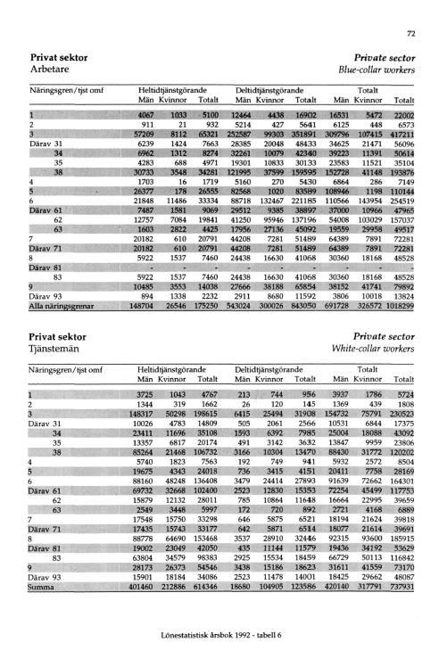
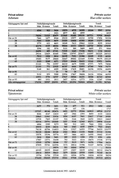
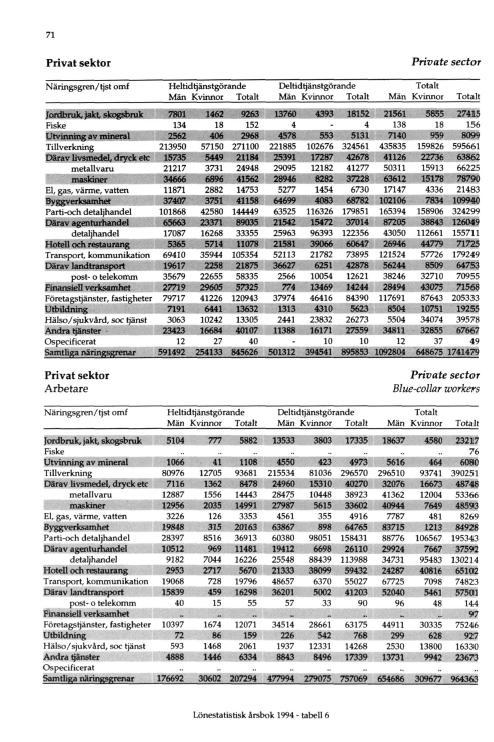
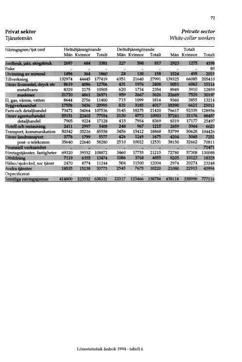
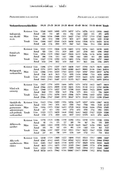
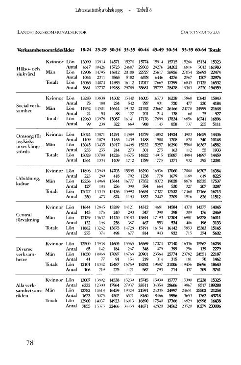
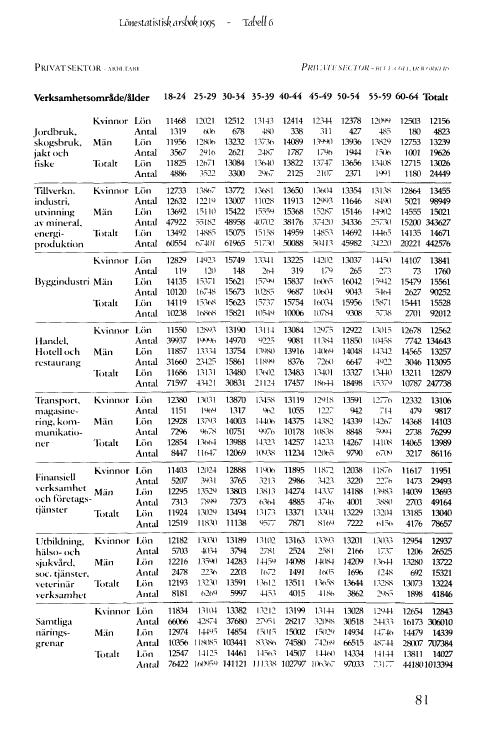
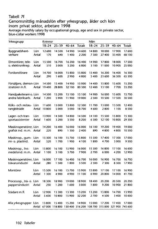
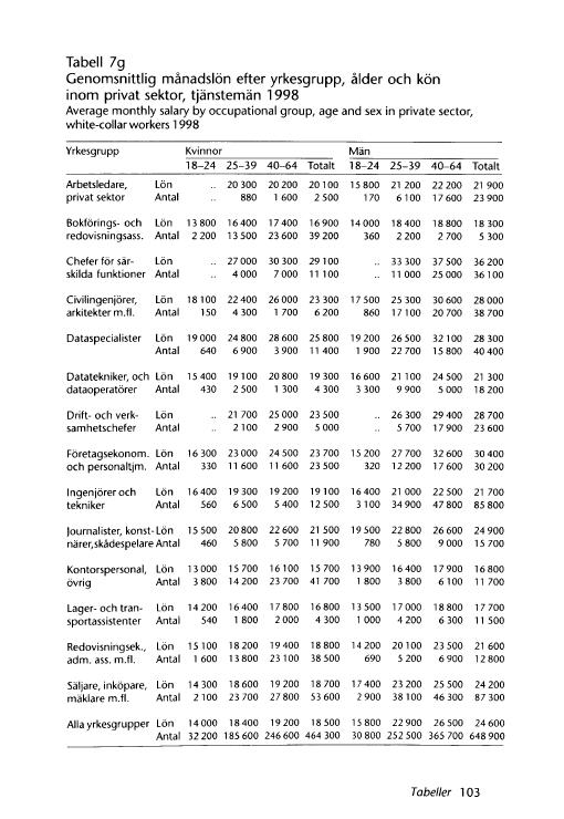
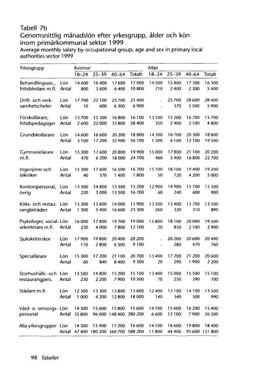
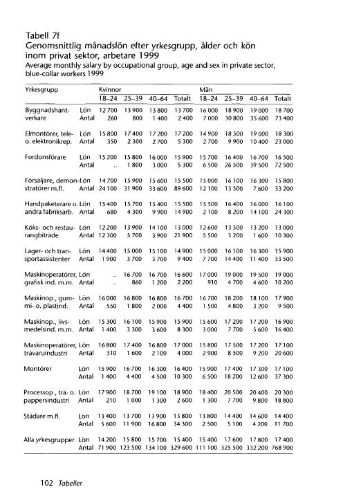
21 The fertility rate has been studied between 1947 and 2010 in order to get the aggregated fertility for all age groups. A 64 year old worker in 1992 entered the labor market in 1948 which means that every day since is a potential days for OTJ minus all days parental leave. What we see in the statistics is that the total fertility rate has declined over time with temporary rises and falls. Another structural change is that the average ages of having the first child have been higher in 2010 than ever before. Under the last four decades the fathers have been about 3 years older than the mothers, so the probability of paternity is assumed to be the same as the fertility rate for the three years younger women for the whole time period Sector As additional explanatory variables I have chosen sectors: the public sector which is split into the state, county council and municipal and the private sector which is divided into white collar and blue collar work. Besides sectors being included in earlier research it also has the interesting feature because of the extensive segregation on the Swedish labor market. Women dominate occupations in the county council and in the municipal where healthcare, day-care and primary school teaching is included while men dominate both parts of the private sector. Partly the segregation probably is an expression of the genders having different preferences, valuing diverse job characteristics differently and therefore find their highest utility, on average, in different sectors. The trend since 1992 is a rising share of women working in the private sector the rise is cause by two effects. The first effect is that the private sector has relatively the public sector grown during the period. The other effect is a higher share of females working in the white collar sector from around 20% in 1992 to about 30% in During the same period the share of women working in the blue collar sector did not change at all 7. In total this means that circa half of the women worked in the private sector in Despite the increase women is still underrepresented within the sector because about 83% of all working men were at the same year employed within the sector (starting at 73% in 1992). This means that the segregation in the private/public case have been somewhat lower. Diagram 4 and 5 shows the average monetary wage for workers between by sector. 7 Own calculations with data from SCB Database, see separate excel file. 17

22 Diagram 4 Diagram 5 For men the county council and the private white collar are the highest paying sectors followed by the state which all are above the average. The municipal and the private blue collar sector is the lowest paying far below the average wage. For the women the series shows 18

23 that private white collar sector together with the county council and governmental work is the most lucrative sectors. The municipal and the private blue collar jobs are below the average. We can summarize this information into three important conclusions: (1) The private blue collar and the municipal sector has paid a lower wage for both genders. (2) The private white collar, the state and the county council has paid a higher wage than average. (3) In all sectors the average wage of men has been higher. Another important fact not captured by the diagram is that the private sector is higher paying for both women and men, between the difference was approximately 2.5% for men and 5% for women 8. The explanatory variable sector is simply the percentage share of the cohort: 3.2 OLS Within econometrics seven assumptions has to be fulfilled to make the Ordinary least squaremethod to be the best unbiased estimator. They state that the regression model is linear with an additive error term that has a mean of zero, is uncorrelated with the explanatory variables and other observations of the error term, has a constant variance and is normally distributed (Studenmund, 2011). Best, in this case, means producing estimates with a minimized sum of squared residuals. When evaluating the estimates one of the criteria s is how good the overall fit is. The fit is a number between 0 1 where close to 1 indicates a great fit. It is calculated by subtracting 1 by the sum of the squared residuals divided by the total sum of squares: Because adding independent variables (K) into the equation never decrease use the adjusted r squared which corrects for the degrees of freedom: it is better to Besides the t-test is a compulsory part of the evaluation. The T-test show how sure it is that the β-coefficient is significantly different from zero. When testing schooling, OTJ and the 8 Own calculations with data from SCB Database, see separate excel file. 19

24 rest of the independent variables the aim is to prove that they are significant in the expected direction Multicollinearity Perfect multicollinearity is a problem where the OLS is unable to accurately estimate the coefficients of the true model. The cause is a violation of the assumption of no explanatory variable being a perfect linear function of one or more of the other explanatory variables (Studenmund, 2011). When including all possible sectors as explanatory variables 10 and measure the share of them, one explanatory variable will be the remaining percent of the share of workers that not is employed in any other sector. When not all sectors are included we are able to avoid the problem of perfect multicollinearity but still the different employment shares are correlated and the OLS will get the problem of imperfect multicollinearity. The consequences will be unreliable estimates with high standard errors; therefore the sectors will be tested once at the time in five otherwise equal regression models for both genders Omitted variable Before running a regression it is important to include all variables that substantially affect the dependent variable and to not leave any outside the function. The variables chosen are motivated by economic theory and earlier research results which also suggest occupation as a relevant factor (MI, 2011). Leaving an important variable outside the function means not holding it constant when running the regression. For example if we have: And exclude OTJ from the equation, we got: But actually we have: This bias is stronger the more correlated the omitted variable are with the included variable. This breaks the third classical assumption because the explanatory variable is no longer uncorrelated with the error term. After reading earlier research of the MI who also omitted the variable in their latest publication without reporting about any risk of serious bias (MI 2011) getting fairly 9 In part 3.3 all expectations is summarized. 10 With exception for parishes of the church of Sweden where 0.6% of the total labor force were employed during the 90 s until the split with the state in Source: Own calculations with data from statistical yearbook of SCB. ( ) 20

25 good fit I chose to not include different occupations in the function. In the same report they tried to add occupation with a better fit as result. This is the unavoidable outcome for my regressions too but as long no bias appears both the primary and secondary aim can still be reached. 3.3 Regression models Now when all variables are presented it is time to build the complete regression functions for both genders 11. To avoid perfect and severe multicollinearity just one sector will be in the function at the time. These pairs of regressions will primary be used to check if we can reject the null hypotheses of the sectors themselves. I will also create one pair of functions without any sector and one pair with the aggregated private sector. Both will be used to measure the impact of inequalities of the parental leave on the wage gap, the latter will also be used in explaining the effect of the imbalances between the genders in private sector. The functions have got the following expressions: Model 1&2b Model 1&2c Model 1&2d Model 1&2e Model 1&2f Model 1&2g 11 Separate regressions for the genders are used, equal in every aspect except the difference in the Pot OTJ definition. Models for men are named 1[letter] and models for women are named 2[letter]. 21

26 3.4 Expectations So far this paper has examined a good deal of theoretical input seeking to explain the wage determinants, especially of human capital accumulation. The main focus has been on education and OTJ. In section 2.2 the Mincer earnings function showed how education raise wage and how OTJ do the same but is diminishing. It has also stressed relevant statistics for the earlier variable, over fertility rates and the withdrawal of the parental leave which influences the second. Further six additional variables, all sectors, have been added. The selection has been made after consideration of reading earlier studies that have found sector to be a central wage determinant. In section 3.1 we saw distinct gaps between the sectors. Our theoretical and statistical lesson gives us the following expectations of the selected variables for both genders presented in Table 5. Table 3 4. Estimates In this chapter first the results of the separately regressions will be discussed, starting with the men and continuing with the women. Comparisons are made in order to investigate similarities and distinctions. Afterwards the OTJ coefficients will be used to estimate to what extent the higher absence from work of mothers due to inequalities is the parental leave contribute to the gender wage gap. Finally the effect of the participation differences in the private sector is estimated. 22

27 4.1 Estimates of Models 1a-e Table 4 The five multivariable regressions all show a significant positive relationship between wage and β 1 schooling 12. The coefficient varies between 5 and 9.4% which means that every year of schooling raise the future wage in the corresponding dimension. The relationship between wage and potential OTJ is also significantly positive with a β 2 coefficient in the range of 1.3 and 2.3%. The β 3 indicates the wage is a concave function of potential OTJ, thus the coefficient vary between -0.3 and These three findings are taken all together perfectly in line with the expected signs of the coefficients stated in human capital theory. The interpretations is that human capital accumulation is valuable both when it is gained in school and on-the-job. The concavity of the OTJ is predicted because of the minor investments of elderly workers. From an alternative cost perspective the workers are rational investing more in OTJ when still have time enough to gain from their effort. 12 See appendix for complete regression results. 23

28 The β 4 and β 8 coefficients shows that for every percentage increase of men working in the municipal or the private blue collar sector lower their median wage with 0.7 and 0,3 %. Contrary, a percentage increase of the share of men working in the private white collar sector the median wage rising with 0.4%. The results were predicted and significant at the 95% level. Two of the coefficients, β 5 and β 6, was insignificant. The estimate of employment in the State had the expected positive effect but surprisingly the county council sector had not. A possible explanation for failing to show a positive relationship between wage and percentage working within the state may be the relatively small gap between the median wage of all male workers and those within the sector. The negative correlation of β 5 is probably due to that the county council is the smallest sector for male workers with fewer than 3% of the total employed men. The standard deviation is over seven times bigger than in the private sector where the majority of the men is employed. good fit of the data. The adjusted r square is between 91.9 and 93.6% and can be interpreted as a 4.2 Estimates of Models 2a-e Starting the evaluation of the female coefficients in numerical order, the β 1 is significant positively related to the extent of 6.6 and 8.5%. This gives a possible economic explanation of Swedish women being very well educated. The β 2 is also positive in the range of 1.3 to 1.9% indicating a gradual increasing wage due to human capital accumulation on-the-job. The coefficient of OTJ 2 is significant, just as the β 2, and negative to a small grade, from -0.2 to

29 Table 5 The many employed female workers in the municipal sector lower the median wage for the gender according to our estimate of -5.5%. Survey the Model 2d the opposite effect is found for private white collar work. The positive effect is estimated to be 2.8% and is significant similar to the coefficient for municipal sector. We also find three insignificant estimates of β 5, β 6 and β 8. The signs of β 6 and β 8 are expected while β 5 are more surprising but because of the insignificance carefulness in the interpretation is needed. All three seem to have a weak impact on the wage. The state is expected to have a weaker positive impact on wage than the white collar sector which is the case. Likewise as for the men the sector with the lowest share of the women population also had the highest standard deviation. The state followed by the county is the smallest female sectors. The coefficient of blue collar sector gives the impression that the impact of blue collar jobs is negative but not affecting the average wage a lot, this cannot be explained by 25

30 pure chance though the participation in the sector is high and the standard deviation is the lowest. women too. The r-square adjusted is in the range of 89.6 and 90.8 signaling a good fit the 4.3 Estimates of Models 1f-g and Models 2f-g In order to make precise comparisons between the genders two pair of equations is created. The pair denoted f is made to compare the return of schooling and the potential OTJ and by the estimated coefficients test how much of the wage gap is attributable to inequalities in potential OTJ. The subsequent pair of models is used to measure the impact of inequalities belonging to sector. Model 1f and 2f is including the three explanatory variables that builds the foundation for the earlier regressions. The regressions have a strong reliability because they are examples of the base of the Mincers earning function with a small adjustment for the absence from work during parental leave. All coefficients pass the 99% significance level. On the basis of the information in the upper columns is it clear that the men have a higher intercept meaning a higher entry wage without any investment in human capital. Table 6 Because of the rareness of having less than 9 years of schooling on the Swedish labor market the intercept cannot be investigated separately leading to any important conclusions of the real 26

31 situation. The β2 s have a small difference, 8.73% is the return for the men and 8.82% for the women. This means that after 10 years of schooling the wage increase of men is 131% compared to the wage paid to men without any education, for women the increase is 133%. However, this higher increase does not compensate for the lower intercept. After 10 years of schooling the wage difference is 13.4% and 13.1% after 5 additional years. Even if a women major continuing taking a PhD (21 years of schooling) the entry wage is still 12.6% lower than for the male students. Transforming the wage gap into educational time approximately 1.7 years is needed to close it totally. The difference in the average time of schooling of the genders was 0.05 years in 1992 and 0.49 years in Given our estimates a further dispersion of 1.2 years should close the entry wage gap. It is important to remember the segregation in the educational attainment among gender. The choice of what topic to study and where to do it is not empirical researched in this thesis but it should play an important role of determining the future earnings. With the same composition of education at institutions with the same quality an increase of average female educational attainment of 1.2 years up to 13.8 years should compensate for entry differences. When inspecting the return to potential OTJ a higher deviation of the coefficients is found. The yearly return of men is 2.1% and for women 1.4%. Graphically speaking the return is also more concave for the men. The interpretation is that the gain of human skill accumulation of post-school investments is higher but also is taping of faster for men. The peak is reached after 39 years of potential OTJ and during the remaining active years more accumulation result in a slightly negative effect on wage. As explained in the theory chapter old workers should invest less in OTJ because of their relatively low marginal revenue. What our empirical result tell us is that the opportunity cost after 39 years of potential OTJ for men is larger for all positive numbers of OTJ so every day invested is non profitable. The lower taping-off effect for women indicate a positive return to OTJ for all active years. After 23 years of OTJ the positive effect on wage is equal for the genders, during the earlier years the wage increase is, in percentage, higher for men and in the subsequent the wage development is greater for women. Now the analysis has brought us all sufficient information able us turning to the main question of how much of the gender wage gap is attributable to inequalities in parental leave. The average real gender wage gap over the whole period for all age groups was 16.4%. To see how much the higher absence from work of the mothers is affecting the gap new values of potential OTJ and OTJ 2 is created. It is done by setting the withdrawal of the parental leave equal for all years studied. These numbers are used as inputs together with the 27

32 average length of schooling in Models 1f and 2f. The remaining wage gap after correcting for parental leave is 15.9%. Thus after the correction 97.2% of the wage gap remains leading to the conclusion that 2.8% of the gender wage gap is caused by the parental leave inequalities. Our secondary question to answer how much of the wage gap can be derived from employing sector. As shown in Table 4 and 5 private white collar jobs has the highest positive effect on wages for both genders and municipal employment has the largest negative effect. It had been optimal to include all five sectors in analyzing this question but since the problem of severe multicollinearity occurs when more than one independent variable is a function of another independent variable this would not lead to reliable estimates. To get around the problem Model 1g and 2g is created. As a new explanatory variable the participation in private sector jobs of every age group for every year is aggregated. In part 2.1 data from SCB pointed out that the private sector is paying better than the public for both women and men even though the wage spread within the sector is large. Further it is shown that women have been underrepresented in the private sector with about half the population employed compared to men where all age groups never had a lower share than two-thirds employed within the sector. In Table 6 a positive relationship between wage and the percentage working in private sector is indicated by the β 9 coefficients of 0.7 men and 1.9 for the women. The low effect for men is contributory to the insignificance while the coefficient for women is significant at the 90% level. To find the magnitude of the effect on wage from participation in the private sector the real wage gap is compared to the wage gap after setting female participation the level of men for all age group for all years 13. Of the initial 16.4% gap 10.9% is left after the correction. It means that 33.3% is explained by employing sector. But this estimate has to be treated very carefully. First the two highest significance levels were not fulfilled of the private sector coefficient. Secondly, the addition of this variable did not raise the r-squared adjusted, making it harder for us to believe that this variable should have such a strong the explanatory power of the wage gap. Section stressed what happens if an omitted variable are correlated with an independent variable inside the equation; bias occurs. Unfortunately sector is the most likely variable to be correlated with occupation. When all these bells are ringing we do not have confidence to say that the question has been answered properly. In order to check the robustness of the estimate of equal parental leave a test with the equal take-up numbers and the coefficients from Model 1g and 2g is done. The 13 The reason why the level of men employed in the sector, and not vice versa, is held constant is because no farreaching conclusions can be done by using insignificant estimates. 28

33 result is that 37.8% of wage gap can be explained by share working in the private sector and equal parental leave together. Subtracting the stated estimate of employing sector, 4.5% is left, 1.7 percent higher than the original estimate. The equal take-up numbers is also tested using the real share employed in private sector leading to a remaining 4.9% of the initial wage gap, 2.1% percent higher than our original estimate. The test serve as a sensitivity analysis and confirms that inequalities in parental leave do not play a major role of the gender wage gap the last two decades Summary and conclusion This thesis has, encouraged by the American study of Budig and England, aimed to inspect the gender wage gap on the Swedish labor market in order to find out if inequalities in the withdrawal of the parental leave have been an important contributor. I created a modified version of the Mincer earnings function with the variable on-the-job training (OTJ) subtracted by the average time of absence from work due to parental leave. In order to estimate the effect statistics over fertility rates, educational level and the length of the take-up of each gender was collected, processed and presented. Important finding made from processing the data is that women on average have become better educated than men during the period, with a difference of approximately a half year in 2010 and the tendency is that the educational gap is widening. What also can be told from the data is that Sweden has become more equal in both the withdrawal of the parental leave at the same time the wage gap has tightening slightly. Before 1974 all the care-taking of the new born was the mothers job, in 2010 the take-up was 77-23%. The relationship between wage and potential OTJ is found positive for the first 39 years for men and for all years of the working life of women. The structure of this compensation is higher for men under the first half of the working life and lower during the second. The return to schooling has been estimated to yield a yearly positive return of % for men and % for women. The estimate of the effect of the inequalities in the parental leave is 2.8%. The sensitivity test showed that the estimate did not change much when trying an alternative regression model. Based on theory, significance and fit it can be concluded that the parental leave inequalities has not been an important contributor the gender wage gap. 14 For the same reasons as previous when using the Model 1g and 2g we should be extra careful. 29

34 The segregation of employing sector has been substantial but decreasing. A positive relationship between wage and share working in the private white collar sector is found while the share working in the municipal has a negative effect on wage for both genders. The underrepresentation of women in the overall private sector is estimated to explain 33.3% of the wage gap but might be upward biased by the omitted variable occupation. As a last note the tightening of the gender wage gap is believed to be caused by a mixture of comparative better education of women and a larger share of women working in the private white collar sector and modestly of a more equal parental leave withdrawal at the end of the period. 6. References 6.1 Literature Becker, G. S.(1962), Investment in human capital: A theoretical analysis in Journal of Political Economy, vol 70, no 5, pp The University of Chicago press. Available [online]: [ ] Becker, G. S.(1975), Human capital: A theoretical and empirical analysis, with special reference to education, 2 nd ed, for National Bureau of Economic Research. Available [online]: [ ] Borjas, G.(2008), Labour economics, 4 th ed., pp. 215, 217 & 248-, McGraw-Hill, New York, 2008, ISBN: Borjas, G.(2010), Labour economics, 5 th ed., pp , McGraw-Hill, New York, 2010, ISBN: Budig, M. J., England, P.(2001), The wage penalty for motherhood in American Sociological Review, vol 66, no 2, pp Available [online]: [ ] Meyersson, E. M., Petersen, T., Snartland(2001), Equal pay for equal work? Evidence from Sweden and a comparison with Norway and the U.S in The Scandinavian Journal of Economics, vol. 103, pp Available [online]: [ ] Mincer, J.(1974), Schooling, experience and earnings in Columbia University Press, 1974, for National Bureau of Economic Research, pp Available [online]: [ ] 30

35 Mincer, J., Jovanovic, B., (1982), Labor mobility and wages, working paper no 357, for National Bureau of Economic Research. Available [online]: [ ] Morgan, L. A., Petersen, T. (1995), Separate and unequal: Occupation-establishment sex segregation and the gender wage gap in American Journal of Sociology, vol 101, no 2, pp Available [online]: [ ] National Mediation Office (MI), (2011), Om löneskillnaden mellan kvinnor och män, Stockholm. Available [online]: [ ] Nyberg, A.(1989), Tekniken kvinnors befriare? Hushållsteknik, köpevaror, gifta kvinnors hushållsarbetstid och förvärvsdeltagande 1930-talet 1980-talet, Tema T, Linköping, ISBN: Schultz, T. W.(1961) Investment in human capital in The American Economic Rewiew, vol 51, no 1, pp Available [online]: [ ] Smith, A. (1776/2007), Den osynliga handen Adam Smith i urval, pp , Timbro, Stockholm, [Original title: The wealth of nations] ISBN: Studenmund, A. H.(2011), Using econometrics, 6 th ed., Pearson Internation ed., 2011, ISBN-13: Svensson, L.(1995), Closing the gender pay gap, Lund University: Departement of Economic History, Lund, ISBN: Waldfogel, J.(1997), The effect of children on women s wages in American Sociological Review, vol 62, no 2, pp Available [online]: [ ] Waldfogel, J.(1998), Understanding the family gap in pay for women and children in Journal of Economic perspectives, vol 12, no 1, pp Available [online]: [ ] 6.2 Other sources Riksbank, The central bank of Sweden, website. Available [online]: [ ] Statistics Sweden (SCB), Personal contact with Michael Karlsson,

36 6.3 Statistics Statistics Sweden (SCB), (2002), På tal om kvinnor och män lathund om jämställdhet 2002, Stockholm. Available [online]: [ ] Statistics Sweden (SCB), (2010a), Women and men in Sweden facts and figures 2010, Swedish title: På tal om kvinnor och män lathund om jämställdhet 2010 SCBtryck, Stockholm, ISBN: Available [online]: [ ] Statistics Sweden (SCB), (2010b), Educational attainment of the population 2010, Örebro. Available [online]: M1101.pdf Statistics Sweden (SCB), (2011a), Database. Available [online]: [ ] Statistics Sweden (SCB), (2011b), Database. Available [online]: 4ssor.pdf [ ] The Swedish Insurance Agency (former), (FK), (2004), Föräldrapenningen - Statistik information. Available [online]: [ ] World Bank, (2012), World development indicators: Labor participation rate female (% of female population ages 15+). Available [online]: [ ] 32

37 Appendix Complete regression results from Table 4 Complete regression results for the regressions made in Table 4 all made in Excel. 33

38 34

39 4.2.1 Complete regression results from Table 5 Complete regression results for the regressions made in Table 5 all made in Excel. 35

40 36

41 37

42 4.3.1 Complete regression results from Table 6 Complete regression results for the regressions made in Table 6 all made in Excel. 38

43 39

44 Supplement Supplement 1 - Employed by sector The following statistics are collected from Statistical yearbook of This is the numerical base for my calculations of sector share. 40

45 41

46 42

47 43

48 44

49 45

50 46

51 47

52 48

53 49

54 50

55 51

56 52

57 53

58 54

59 55

60 56

61 57

62 58

63 59

64 60

65 61

66 62

67 63

68 64

69 65

70 66

71 67

72 68

73 69

74 70