Catalonia: Independence and Pensions. May 11, 2017

Transcription

1 Catalonia: Independence and Pensions Javier Díaz-Giménez IESE Business School Julián Díaz-Saavedra Universidad de Granada May 11, 2017 Abstract This article confirms and quantifies the intuition that the consequences of independence for Catalonian residents will depend crucially on the long term growth rate of the new republic. It also shows that the demographic, educational, and productivity advantages of Catalonian residents, when compared with those of the rest of Spain, are not enough to ensure a more prosperous economic future for Catalonians or a more sustainable pension system. Keywords: Computable general equilibrium, social security reform, retirement JEL classification: C68, H55, J26 We thank Juan Carlos Conesa for an early version of the code. We are also grateful to Jesús Díaz Díaz, who suggested that we should research this topic.

2

3 1 Introduction Catalonian residents are trying to decide whether to become independent from Spain. If they choose to remain in Spain, the future of their economy and of their pensions will remain connected to the future of the Spanish economy and of Spanish pensions, which we have analyzed recently in Díaz-Giménez and Díaz-Saavedra (2017). If they choose to become independent the future of their economy and of their pensions will depend on the decisions they make and on the type of pension system that they adopt. In this article we study the future of the pension system in an independent Catalonia, assuming that they decide to replicate the current Spanish pension system. Three factors will condition the future of Catalonian pensions: the demographics, the productivity, and the education of its residents; the severity and the duration of the post-independence recession, which would most likely result from a disputed seccession; and the long-term growth rate of the new Republic of Catalonia. The trade-off: Catalonian residents are younger, more educated, and more productive than the residents in the rest of Spain. These three features would make any Catalonian pension system more sustainable, if Catalonia were to become independent. But these features have to be traded-off quantitatively against the reduction in payroll tax revenues and increases in the pension expenditures to output ratio, that will result from the post-independence recession. The questions: In this article we ask the following two questions: if independence were to result in higher, long-term growth rates for Catalonia, what would the future of its pension system be? and if an independent Catalonia ended up growing at the same rate as Spain, would the greater youth, education, and productivity of its residents suffice to compensate for even a mild post-independence recession? The Model Economies: To answer these questions, we use a general equilibrium overlapping generations model economy to take a careful look at the consequences for future Catalonian pensions of various growth scenarios for an independent Republic of Catalonia, assuming that the pension system of the new republic is identical to the current Spanish pensions system. To this purpose, we do the following: First, we simulate the Spanish economy after the 2011 and 2013 pension system reforms. This is our benchmark model economy and we call it Model Economy ESP. Then, we take the sequences of prices and tax rates from this model economy and we use them to carry out a partial equilibrium simulation of Catalonia, if it were to remain in Spain. We call this economy Model Economy CAT0. Next, we assume that Catalonia becomes independent from Spain in 2021, and we follow Young (2013) to simulate three growth rate scenarios for an independent Republic of Catalonia according to the severity of the post-independence recessions and the size of the long-run growth rates. We call these Model Economies CAT1, CAT2, and CAT3. In Model Economy CAT1 we simulate a 1

4 mild recession and a high long-run growth rate, in Model Economy CAT2 we simulate a more severe recession and a medium long-run growth rate, and in Model Economy CAT3 we simulate a mild recession and a long-run growth rate that is the same as the Spanish growth rate. Finally, we use these model economies to quantify the aggregate, distributional and welfare consequences of independence placing a special focus on the consequences of independence for pensions. Our model economies are versions of the general equilibrium, multi-period, overlapping generations model economy with heterogeneous households described in Díaz-Giménez and Díaz-Saavedra (2017). The main features of this model economy are the following: the households differ in age, education and employment status, and, consequently, in income, wealth, pension rights, and pensions and they decide optimally how much to work, consume, and save and when to retire. Production is carried out by a neoclassical representative firm that behaves competitively in its product and factor markets. We also model a government that runs a fully explicit and detailed pay-as-yougo pension system financed with payroll taxes, and that uses consumption, capital, and income taxes to finance exogenous sequences of government expenditures and public transfers other than pensions. The Findings: Our results confirm that average pensions would be higher in an independent Catalonia as long as it succeeds in growing at a higher rate than Spain. They also suggest that, if Catalonia only manages to grow at a similar rate than Spain, the higher productivity, higher education, and better demographics of Catalonian residents would only make average pensions higher in an independent Catalonia in the very long run, after We also find that even in the cases where independence would lead to higher long-run economic growth, transition costs may offset these benefits for several years. We also find that the upper bound on the Spanish Pension Revaluation Index is a bad idea. This bound limits the yearly real growth rate of pensions to 0.5 per cent. In the long run it is a bad idea because it is much smaller than the expected average real growth rates of either the Spanish or the Catalonian economies and, consequently, it results in reductions in the pension replacement rates and in pension system surpluses that cannot be justified in welfare terms. 2 The Model Economy We study an overlapping generations model economy with heterogeneous households, a representative firm, and a government. Our model economy is an enhancement of the model economy described in detail in Díaz-Giménez and Díaz-Saavedra (2009). For the sake of brevity, we offer only a brief summary of its main features here. A detailed description of this model economy can be found in the technical appendix to this paper that is available at pen5-app.pdf. 2

5 2.1 The Households Households in our model economy are heterogeneous and they differ in their age, in their education, in their employment status, in their assets, in their pension rights, and in their pensions. Age. Households enter the economy at age 20, the duration of their lifetimes is random, and they exit the economy at age 100 at the latest. Fertility and Immigration. In our model economy fertility rates and immigration flows are exogenous. Education. Households can either be high school dropouts, high school graduates who have not completed college, or college graduates. A household s education level is determined forever when it enters the economy. Employment status. Households in our economy are either workers, disabled households, or retirees. Every household enters the economy as a worker, and every worker faces a positive probability of becoming disabled. Once a household has reached the early retirement age, it decides whether to retire. Both the disability shock and the retirement decision are irreversible and there is no mandatory retirement age. Workers. Workers receive an endowment of efficiency labor units every period. This endowment has two components: a deterministic component and a stochastic component. The deterministic component depends on the household s age and education, and we use it to characterize the lifecycle profiles of earnings. The stochastic component is independently and identically distributed across the households, and we use it to generate earnings and wealth inequality within the age cohorts. Disabled Households. Each period, workers face a probability of becoming disabled. When this happens, the worker exits the labor market and receives no further endowments of efficiency labor units, but she is entitled to receive a disability pension while she is alive. Retirees. Retirees do not receive an endowment of efficiency labor units, but they receive a retirement pension. Insurance Markets. A key feature of our model economy is that there are no insurance markets for the stochastic component of the endowment shock. When insurance markets are allowed to 3

6 operate, every household of the same age and education level is identical, and the earnings and wealth inequality is greatly reduced. Assets. Households in our model economy differ in their asset holdings, which are constrained to beingnon-negative. Since leisure is an argument of their utility function, this borrowing constraint can be interpreted as a solvency constraint that prevents the households from going bankrupt in every state of the world. These restrictions give the households a precautionary motive to save. They do so accumulating real assets which take the form of productive capital. Pension Rights and Pensions. Workers differ in their pension rights and disabled households and retirees differ in their pensions. Workers accumulate pension rights when they pay payroll taxes. These rights are used to determine the value of their pensions when they retire. The pension system design specifies the rules that govern the accumulation of pension rights, and the rules that determine the mapping from pension rights into pensions. In our model economy workers take this mapping into account when they decide how much to work, how much to save, and when to retire. Preferences. Households derive utility from consumption and from non-market uses of their time, and their preferences can be described by the standard Cobb-Douglas expected utility function that we define in Expression (21). 2.2 The Firm In our model economy there is a representative firm. Aggregate output at period t, Y t, depends on aggregate capital, K t, and on the aggregate labor input, L t, through a constant returns to scale, Cobb-Douglas, aggregate production function of the form Y t = K θ t (A t L t ) 1 θ (1) where A t denotes an exogenous labor-augmenting productivity factor whose law of motion is A t+1 = (1 + γ t ) A t, and where A 0 > 0. Factor and product markets are perfectly competitive and the capital stock depreciates geometrically at a constant rate, δ. 2.3 The Government The government in our model economy taxes capital income, household income and consumption, and it confiscates unintentional bequests. It uses its revenues to finance an exogenous flow of public consumption, and to make transfers other than pensions to households. The government also runs a pay-as-you-go pension system, which we describe below. The consolidated government and pension 4

7 system budget constraint is G t + P t + Z t = T kt + T st + T yt + T ct + E t + [(F t (1 + r ) F t+1 ] (2) where G t denotes government consumption, P t denotes pensions, Z t denotes other government transfers, T kt, T st, T yt, and T ct, denote the revenues collected by the capital income tax, the payroll tax, the household income tax, and the consumption tax, E t denotes unintentional bequests, F t > 0 denotes the value of the pension reserve fund at the beginning of period t, and r denotes the exogenous interest rate that the government obtains from the pension reserve fund assets. Consequently, [F t (1 + r ) F t+1 ] denotes the revenues that the government obtains from the pension reserve fund or that deposits into it. We assume that the sequence of government consumption is exogenous, that government transfers other than pensions are thrown to the sea so that they create no distortions in the household decisions, that unintentional bequests are confiscated, and that the pension reserve fund is nonnegative. Capital income taxes. Capital income taxes are described by the following function τ k (y k t ) = a 1 y k t (3) where y k t denotes before-tax capital income. Household income taxes. To model the household income tax, we use the following function: [ ] } τ y (yt b ) = a 2 {yt b a 3 + (yt b ) a 1/a4 4 (4) where yt b is the income tax base which we define as follows: yt b = yt k + yt l + p d t (b t ) + p t (b t ) τ s (yt) l τ k (yt k ) (5) In these expressions, yt k is before-tax capital income, yt l is before-tax labor income, p d t is the disability pension, p t is the retirement pension, τ s and τ k are the payroll tax and the capital income tax functions, that we describe below, and a 2, a 3, and a 4 are parameters. Expression (4) is the function chosen by Gouveia and Strauss (1994) to model effective personal income taxes in the United States, and it is also the functional form chosen by Calonge and Conesa (2003) to model effective personal income taxes in Spain. Consumption taxes. Consumption taxes are described by the function τ c (c t ) = a 5t c t. (6) 2.4 The Pension System To complete the specification of our model economy we need to describe its pay-as-you-go pension system. A pay-as-you-go pension system is a payroll tax, the rules that govern the accumulation 5

8 of pension rights, and the rules that map pension rights into pensions. These rules include the rules that specify the legal retirement ages and the rules that describe the revaluation of pensions. In our benchmark model economy we choose the payroll tax and the pension system rules so that they replicate as closely as possible the Spanish pay-as-you-go pension system in 2014, which is our chosen benchmark model economy calibration year. Retirement Ages. In Spain in 2014 the retirement age that entitled workers to receive a full retirement pension was 65 for the workers who had contributed during at least 35 years and 6 months. Workers with a shorter contributive period were required to retire at 65 years and two months. Workers aged 61 or older could retire earlier paying an early retirement penalty, as long as they had contributed to the pension system for at least 30 years, and when the decision to retire had not been made by the worker. Workers who decided to retire voluntarily were required to be 63 years and two months old, as long as they had contributed to the pension system for at least 35 years. The 2011 and 2013 Pension Reforms delayed these legal retirement ages gradually. This delay will be completed in 2027 when the normal retirement age will reach 67 and the minimum retirement age will reach In our model economy the early retirement age is R 0 and the normal retirement age is R 1. In 2014 these ages are 61 and 65 years. We delay the legal retirement ages to 62 and 66 years in 2018, and to 63 and 67 years in See Díaz-Giménez and Díaz-Saavedra (2016) for the details. Covered Earnings. The Spanish pension system puts a limit on pensionable earnings. Therefore, in many cases, the earnings covered by the pension system are less than the actual earnings. In our model economy we denote the covered earnings by ŷit l, and we define them as follows: ŷ l jt = min{y l jt, y max,t } (7) where y max denotes the maximum covered earnings. We model maximum covered earnings as a constant proportion, a 6, of per capita output at market prices at every period t. Formally y max,t = a 6 ȳ t (8) Payroll Taxes. In Spain payroll tax rates are proportional to covered earnings, which are defined as total earnings, excluding payments for overtime work. In 2014 the payroll tax rate was 28.3 percent, of which 23.6 percent was attributed to the employer and the remaining 4.7 percent to the employee; maximum monthly covered earnings were 3,198 euros. 2 In our model economy the 1 The early retirement limit will reach 63 years in 2017 for workers whose retirement decision is not voluntary. 2 Covered earnings ceilings vary with broadly defined professional categories. In 2014 there were eleven of these categories, but the effective number of caps was only five. 6

9 payroll tax rate is a 8, and the payroll tax function is the following: ( ) ] τ s (yjt) l a = 7 ȳ t [a 7 ȳ t 1 + a 8yjt l yl jt /a 8ȳ t a 7 ȳ t if j < R 1 0 otherwise (9) where a 7 is the cap of the payroll tax, ȳ t is per capita output at market prices, yjt l is labor income, j is the household s age, and R 1 denotes the normal retirement age. Parameter a 8 controls the slope of the tax function, and we choose its value to match the value of the Spanish payroll-tax collections to output ratio. Early Retirement Penalties. The 2011 and 2013 Pension Reforms established the following early retirement penalties: The early retirement penalties are 7.5 percent per year for households who had contributed between 30 and 34 years; 7 percent per year for households who had contributed between 35 and 37 years; 6.5 percent per year for households who had contributed between 38 and 39 years; and 6 percent per year for households who had contributed for 40 years or more. As we describe below, in our model economy we abstract from the durations of the contributory careers, and workers who choose to retire between ages R 0 and R 1 pay an early retirement penalty, λ j, which is determined by the following function { a9 a λ j = 10 (j R 0 ) if R 0 j < R 1 (10) 0 if j R 1 where a 9 and a 10 are the parameters which we choose to replicate the Spanish early retirement penalties. Specifically, the annual early-retirement penalty is 7 percent per year. The Sustainability Factor. The 2011 and 2013 Pension Reforms also introduce a demographic Sustainability Factor (SF) which will be applied from 2019 onwards. This factor adjusts new pensions to the life-expectancy of cohorts aged 67 so that life-time pension wealth is approximately the same for every cohort. Following the Spanish rules, we assume that the law of motion of the SF is the following: SF t = ε t SF t 1 (11) where ε t is a time-varying measure of the relative life-expectancy at age 67. Specifically, for the period the value of ε will remain constant at ε t = [ ] 1/5 e67,2012 e 67,2017 In this expression variable e 67,t denotes the life expectancy at age 67 in year t. For the period the value of ε will be updated to (12) ε t = [ ] 1/5 e67,2017 e 67,2022 (13) 7

10 and so on. 3 Retirement Pensions. In Spain, at least 15 years of contributions are required to be entitled to receive a contributive retirement pension. In general, these pensions are incompatible with labor income. The method used to calculate the pensions is earnings-based. Pension benefits depend on the amounts contributed, on the number of years of contributions, on the retirement age, and on the values of the Sustainability Factor for first pensions and of the Pension Revaluation Index for all other pensions. 4 In 2014 the regulatory base was defined as the average labor earnings of the last 17 years before retirement. This number will increase gradually one year each year until it reaches 25 years in Taking all this rules into account, in Spain the first pension of a household that retires at age j R 0 is calculated according to the following formula: j 1 p jt = φ(n)sf t (1.03) v (1 λ j ) 1 ŷi,t+i R l N 0 (14) b i=j N b In this formula, function φ(n) denotes the pension system s replacement factor which depends on the number of years of contributions, N, in a way that we have described above; parameter v denotes the number of years that the worker remains in the labor force after reaching the normal retirement age; and parameter N b denotes the number of consecutive years before retirement that are used to compute the retirement pension. In our benchmark model economy we calculate the retirement pensions using the following formula: p jt = φsf t (1.03) v (1 λ j )b jt (15) where b jt denotes the model economy pension rights which we define below. Expression (15) replicates most of the features of Spanish retirement pensions. The main difference is that in our model economy pensions are independent of the number of years of contributions. We abstract from this feature of Spanish pensions for computational reasons. Pension rights. In our benchmark model economy we calculate pension rights so that they replicate the Spanish pension rights as closely as possible. Formally, in the model economy the expression 3 Before 2019 ε t = 1. 4 The pension is 50 percent of the regulatory base when the number of years of contributions is 15, and this percentage increases with the duration of the contributory career. 5 Labor income earned in the last two years before retirement entered into the calculation in nominal terms. The labor earnings of the remaining years were revaluated using the rate of change of the Spanish Consumer Price Index. 8

11 for the value of the beginning-of-period pension rights is the following: j 1 i=j N ŷ b i,t+i R l 0 N b for j = R 0, b jt = (N b 1)b j 1,t 1 +ŷj 1,t 1 l N b for j > R 0, (16) Notice that Expression (16) replicates the Spanish calculation of pension rights exactly for j = R 0 and approximately for j > R 0. In our model economy, as in Spain, N b = 17 in 2014 and then it increases one year each year until it reaches 25 in Minimum and maximum pensions. Spanish pensions are bound by a minimum and a maximum pension. Minimum pensions depend the pensioner s age and on the composition of her household. When an eligible person s pension entitlement is smaller than the minimum pension and she has no other resources, the system tops up her pension entitlement until it reaches the value of the minimum pension. In 2014 the minimum yearly pension was 10,933 euros for pensioners over age 65 with a dependent spouse, and the maximum yearly pension was 35,763 euros. Our model economy introduces this feature. Formally, we require that p min,t p t p max,t (17) where p min,t denotes the minimum pension and p max,t denotes the maximum pension. In our benchmark model economy we revaluate all pensions including the minimum and maximum pensions using the Pension Revaluation Index which we describe below. The Pension Revaluation Index. Until 2013 in Spain minimum and maximum pensions were increased discretionally and all other pensions were revaluated using the Consumer Price Index. Since 2014, all contributive pensions were revaluated according to a Pension Revaluation Index (PRI) which is part of the 2013 Pension Reform. The legal definition of the PRI is the following: g t+1 = g c,t+1 g p,t+1 g s,t+1 + α( R t+1 Ẽt+1 Ẽ t+1 ) (18) where x t denotes the moving arithmetic average of variable x t computed between t 5 and t+5, x denotes the moving geometric average of variable x t computed between t 5 and t+5, g c,t+1 is the growth rate of the pension system revenues, g p,t+1 is the growth rate of the number of pensions, g s,t+1 is the growth rate of the average pension due to the substitution of old pensions by new pensions, 0.25 α 0.33 is an adjustment coefficient, R t+1 denotes the pension system revenues, and E t+1 denotes pension system expenditures. Finally, the Spanish law specifies two bounds for the PRI. The lower bound is 0.25 percent and the upper bound is 0.5 percent plus the inflation rate. In our model economy we replicate the 9

12 formula used to calculate the Spanish PRI exactly and we choose an inflation scenario to replicate its bounds. Disability Pensions. We model disability pensions explicitly for two reasons. First, because disability pensions represent a large share of all Spanish pensions. In 2014, 10.0 percent of all contributive pensions and 14.9 percent of the sum of the retirement and disability pensions paid by the Régimen General were disability pensions. Second, because Spaniards often use disability pensions as an alternative route to early retirement. See Boldrin and Jiménez-Martín (2007) for an elaboration of this argument. The rules used to define pensionable income for workers who qualify for a disability pension in Spain are complex and they depend on detailed individual circumstances and on the type of disability. In our model economy we approximate these rules assuming that the disability pension is 75 percent of the pension rights of the disabled worker and that this amount is bounded below by the minimum retirement pension. Formally, we compute the disability pensions as follows: p d t (b t ) = max{0.75b t, p min,t }. (19) The Pension Reserve Fund. Since the year 2000, Spain has had a pension reserve fund which is invested in fixed income assets and which is financed with part of the pension system surpluses. From 2010 onwards, the reserve fund assets have been used to finance the pension system deficits when needed. In 2014, the total amount of assets accumulated in the pension reserve fund was 41, million euros which corresponded to 4.00 percent of that year s GDP. In our benchmark model economy, we assume that all the pension system surpluses are deposited into a pension reserve fund which evolves according to F t+1 = (1 + r )F t + T st P t (20) We require the pension reserve fund to be non-negative. We assume that the pension fund assets are used to finance the pension system deficits. Once the pension reserve fund runs out, we assume that the government changes the consumption tax rate as needed to finance the pensions. 2.5 The Households Decision Problem The households in our model economy solve the following decision problem: 100 max E β j 20 ψ jt (1 ϕ jh ) [c α jht (1 l jht) (1 α) ] (1 σ) /1 σ j=20 (21) 10

13 subject to c jht + a jht+1 + τ jht = y jht + a jht (22) where τ jht = τ k yjht k + τ y(yjht b ) + τ st(yjht l ) + τ ctc jht (23) y jht = yjht k + yl jht + pd t (b t ) + p t (b t ) (24) yjht k = a jhtr t (25) yjht l = w tɛ jh s t l jht (26) a jht A, p t (b t ) and p d t (b t ) P t, s t ω for all t, and a jh0 is given, (27) and where function τ y is defined in expression (4), variable yjht b is defined in expression (5), function τ s is defined in expression (9), function p is defined in expression (15), and function p d is defined in expression (19). When solving this problem, the households take into account the law of motion of b t, defined in Expression (16), to make theirconsumption, saving, labor and retirement decisions. See Díaz-Giménez and Díaz-Saavedra (2016) for the details. In all these expressions, subscripts j and h denote a household s age and its education level, β > 0 denotes the time-discount factor; ψ jt denotes the conditional probability of surviving from age j to age j+1; ϕ jh denotes the disability shock faced by able-bodied workers; c jht > 0 denotes consumption; we normalize the endowment of productive time to 1; 1 l jht 0 is labor hours; a jht denotes assets; τ ct is the consumption tax rate; and sets A, P t, and ω are finite. Notice that every household can earn capital income, that only workers can earn labor income, that only disabled households receive disability pensions, and that only retirees receive retirement pensions. Consequently, the optimal labor hours of disabled households and retirees are zero. As we have already mentioned, an important feature of the households decision problem that we have omitted from its formal description is that, once they reach the early retirement age, the households in our model economy decide optimally when to retire, taking into account all the benefits and costs of continuing to work and retiring. 2.6 Equilibrium A detailed description of the equilibrium process of this model economy can be found in the on-line technical appendix to this paper. See Calibration To calibrate our model economy we do the following: First, we choose Spain as our calibration target country and 2014 as our calibration target year. Then we choose the initial conditions and 11

14 the parameter values that allow our model economy to replicate as closely as possible selected macroeconomic aggregates and ratios, distributional statistics, and the institutional details of our chosen target country in our chosen target year. More specifically, to characterize our model economy fully, we choose the values of 5 initial conditions and 50 parameters. To choose the values of these 50 unknown parameters, we need 50 equations defined by 50 calibration targets. We determine the values of 31 of those parameters directly either because the equations that determine their values have only one unknown, or because they have one unknown and our guesses for the values of aggregate capital and aggregate labor. To determine the values of the remaining 19 parameters, we solve a system of 19 non-linear equations in 19 unknowns. We describe these steps and our computational procedure in the on-line technical appendix that can be found at 3 Simulation Scenarios To simulate our model economies, we must choose a time period to project our model economies into the future, a demographic scenario, a fiscal policy scenario, a pension system scenario, a growth rate scenario, and an inflation rate scenario. 3.1 Time Period The time period that we consider for our simulations must be long if we want to understand fully the economic consequences of Catalonian independence. Our benchmark model economy is Model Economy ESP and our chosen calibration year is 2014 because it is the last year for which a full dataset is available. Our chosen year for the Catalonian declaration of independence is Of course, this choice is purely metaphorical, we just needed to choose a year that had to be in the near future. We think that a reasonable projection period during which we can safely conjecture that the main institutional features of Spain and Catalonia will remain relatively constant is about 50 years, so that takes our simulation period until Finally we must account for the entire lifetimes of the people who enter the economy between 2021 and We have assumed that people who enter our economy are 20 years old. Therefore, the people who will enter in 2021 were born in 2001 and they may live up to 100, that is until But in the welfare calculations that we describe below we also take into account the welfare of the households who enter the economy between 2021 and The youngest of these households were born in 2050 and they may live until Therefore, our complete simulation period comprises the years between 2014 and This implies that the households whose decisions we are studying were born between 1914 and Our final steady state is in year 2230, but the longest time series that we report in this article end in We 12

15 3.2 Simulating Spain Model Economy ESP: As we have already mentioned, Model Economy ESP is our benchmark model economy, and we calibrate its functional forms and parameters to the Spanish economy. To this purpose, we choose the parameters that describe the preferences, the process on the endowment of efficiency labor units, the disability risk, the production technology, and the components of the government policy so that our model economy replicates as closely as possible the aggregate, institutional, and distributional targets of the Spanish economy in 2014 (see the on-line Technical Appendix for the details). The main features of Model Economy ESP are the following: The Demographic Scenario: We take the sequence of distributions of households by age, {µ jt }, for the period from the demographic projection for the Spanish economy reported by the Instituto Nacional de Estadística (INE). The initial educational distribution replicates the educational distribution reported for Spain in 2014 by the INE. After 2014, we assume that the educational shares for the 20-year old entrants are 7.33 percent, 62.62, and percent forever. Those shares are the educational shares of the most educated Spanish cohort ever, which corresponds to the 1980 to 1984 cohort. Finally, we take the time variant survival probabilities, ψ jt, from the Spanish mortality tables reported by the INE in To project the distribution of households between 2065 and 2150 we use the procedure that we describe in the on-line appendix. The Fiscal Policy Scenario: Recall that the consolidated government and pension system budget constraint in our model economy is G t + P t + Z t = T kt + T st + T yt + T ct + E t + [F t (1 + r ) F t+1 ] (28) In this expression G t is exogenous and the remaining variables are endogenous. We assume that the capital income tax rate and the parameters that determine the payroll tax function and the household income tax function remain unchanged at their 2014 values. We also assume that the consumption tax rates change to finance the pensions once the pension reserve fund has been exhausted. Every other variable in Expression (28) changes with time because they are all endogenous 7. The Pension System Scenario: As we have already mentioned, in our simulation of Spanish pensions we delay the legal retirement ages from 61 and 65 to 62 and 66 years in 2018, and to 63 and 67 years in 2024, and we increase the number of years of contributions taken into account to calculate the pensions from 17 to 25, one year each year between 2014 and We also assume that the maximum covered earnings to output ratio, the payroll tax rate, the parameter that determine the stop there because thinking about 2150 already requires a major feat of imagination. 7 For a detailed account of our calibration of G 2014 see the on-line Technical Appendix that can be found at 13

16 Figure 1: The Spanish Sustainability Factor and Pension Revaluation Index (PRI) A: The Sustainability Factor B: The PRI (%) C: The Accumulated PRI curvature of the social security tax function, and the pension replacement rate remain unchanged at their 2014 values. Finally, we assume that all pensions including the maximum and the minimum pensions are updated yearly using the Pension Revaluation Index (PRI). In Panel A of Figure 1, we plot the values of the Sustainability Factor that we obtain in our simulation of Model Economy ESP. We have computed this factor using the Spanish 2014 mortality tables, and the projection of the Spanish survival probabilities until 2100 that we describe in the on-line appendix. We find that the Sustainability Factor will reduce the value of first pensions by 27.4 percentage points between 2020 and Finally, we assume that every model economy that we simulate in this article has exactly the same Sustainability Factor. This is because it depends exclusively on life-expectancy and, therefore, on survival probabilities, and the Catalonian Institute of Statistics (IDESCAT) does not report a projection of survival probabilities for Catalonia. In Panels B and C of Figure 1, we plot the values of the PRI that we obtain in our simulation of Model Economy ESP. We find that the PRI is negative every year between 2020 and The accumulated PRI shows the reduction in the real value of the pension of a retiree who enters the system in Twenty years later, in 2040, the value of the accumulated PRI will be 88.5 and, therefore, her pension will be will be about 11.5 percent smaller. To calculate the impact of the PRI on the pensions of workers who retire later, the PRI must be renormalized to 100 on the year that they retire. For instance, in 2050 the accumulated PRI of a worker who retires in 2030 will be (= /95.3) and, therefore, her pension will be about 17.3 percent smaller than when she retired. The Growth Rate Scenario: In our model economies there are three sources of output growth: the exogenous changes in the labor-augmenting productivity factor; the exogenous changes in the distributions of households by age and education; and the endogenous changes in consumption, savings, labor hours and, retirement that result from the changes in prices and pensions. In Model Economy ESP, we target a constant two percent output growth rate scenario, for the entire 14

17 period. To achieve this target, we assume that the exogenous growth rate of the laboraugmenting productivity factor is also two percent during this period. The Inflation Rate Scenario: We assume that the yearly inflation rate in our model economies is two percent for the entire period. We choose this scenario because two percent is the inflation rate targeted by the European Central Bank. This inflation rate scenario implies that the real value of the lower bound of the Pension Revaluation Index is 1.75 [= ] and that the real value of its upper bound is 0.5 percent, as established by Spanish law. Figure 2: The Productivity Life-Cycle Profiles in Catalonia and in Spain A: High School Dropouts B: High School Graduates C: College Graduates 3.3 Simulating Catalonia Model Economy CAT0. This model economy represents Catalonia as a part of Spain. To capture this feature, we model it as a partial equilibrium model economy that only differs from Model Economy ESP in the age and education distribution of its households and in the deterministic component of its labor productivity process. Otherwise, Model Economies ESP and CAT0 are identical, as befits to two economies that are integrated. Specifically, Model Economies ESP and CAT0 have identical preferences, technologies, prices, the random components of their labor productivity processes, and the exogenous components of their government policies and of their pension systems, including their maximum covered earnings sequences, their minimum and maximum pension sequences, and their Pension Revaluation Index and Sustainability Factor sequences. Their labor productivity growth rates and their inflation rate scenarios are also identical. The endogenous components of fiscal policy in Model Economy CAT0, which are transfers and unintentional bequests, differ from those in Model Economy ESP but they compensate each other exactly to allow the governments to satisfy their budgets every period. Finally, since the Pension Reserve fund in Model Economy ESP runs out in 2017, we assume that {F t } = 0 for all t in the 15

18 four Catalonian model economies. Model Economies CAT1, CAT2, and CAT3. These three model economies represent independent Catalonia. In all three we assume that independence takes place unexpectedly in 2021 and, as befits independent countries, we model them as general equilibrium model economies. Consequently, their price processes differ from each other and from the price processes in Model Economy CAT0. As we discuss in detail below, these three model economies also differ substantially in their growth rate scenarios. Model Economy CAT1 has a small post-independence recession and a high longrun growth rate. Model Economy CAT2 has a large post-independence recession and a medium long-run growth rate, and Model Economy CAT3 has a small post-independence recession and a low long-run growth rate. But in many other ways our independent Catalonia model economies are similar to each other and to Model Economy CAT0. Specifically, they all have identical distributions of households by age and education, identical deterministic components of their labor productivity processes, identical exogenous components of fiscal policy and of the pension system, and identical inflation rate scenarios. In spite of these similarities, the differences in growth rates generate substantial differences in all the endogenous variables during the first few decades as we discuss below. The Life-Cycle Productivity Profiles: In Figure 2 we plot the deterministic component of the productivity profiles of our three educational groups. These profiles are somewhat higher for Catalan workers than for Spanish workers, because Catalan workers are more productive. According to BBVA (2009), Catalonian workers were 7 percent more productive per hour than their counterparts in the rest of Spain. To model the life-cycle productivity processes we use the following family of quadratic functions: ɛ jh = ξ 1h + ξ 2h j ξ 3h j 2 (29) To increase the productivity of Catalonians we multiply the coefficients ξ 2h and ξ 3h by a factor of 1.07 and we leave coefficients ξ 1h unchanged. We do this for two reasons: first, to highlight that the productivity differences are most likely increasing in education and, second, to make the productivity differences increasing in age. The Age Distribution of Households: We obtrain the sequence of distributions of households by age for our Catalonian model economies from the 2013 demographic projection reported by the Catalonian Institute of Statistics (IDESCAT). In Panel A of Figure 3 we plot the changes in the 65+ to dependency ratios, and in Panels B and C we plot the numerators and the denominators of those ratios. In Catalonia, this ratio increases from 33.1 percent in 2020 to 70.4 percent in 2070 and, in Spain, from 33.3 to As we have already mentioned, we assume that the sequences of survival probabilities in Catalonia and in Spain are the same. 16

19 Figure 3: Demographics and Education in Catalonia and in Spain A: Age Dependency Ratios B: Share of Working Age (20 64) C: Share of Retirement Age (65+) D: Education Shares (Dropouts) E: Education Shares (High school) F: Education Shares (College) The Educational Distribution of Households: We assume that the educational distribution of households in 2014 in our Catalonian model economies replicates the educational distribution of the Catalonian population in 2014, as reported by IDESCAT. Form 2014 onwards, we assume that the educational shares for the 20-year old entrants are 8.53 percent, 57.88, and percent. These shares correspond to the most educated Catalonian cohort ever, which was the 1980 to 1984 cohort. In Panels D, E, and F of Figure 3 we plot the education shares of Dropouts, High School, and College educated households. The shares of High School households are higher in Spain than in Catalonia and the shares of College households are higher in Catalonia than in Spain. The Growth Rate Scenarios: One of the key arguments in the economic discussions about Catalonian independence is its future growth rate scenario. In the short run, almost everyone agrees that independence will result in a post-independence recession. In the long run, the economists that favor independence argue that Catalonia will grow more than Spain, and the economists that oppose independence argue that the long-run differences in growth rates between Catalonia and Spain will be very small. To quantify these scenarios we must answer three questions: (i) how severe will be the postindependence recession; (ii) how long will it last for; and (iii) what will be the long-run growth rate of an independent Catalonia. We are agnostic about the answers to these three admittedly hard questions, so we turned to the literature for guidance. 17

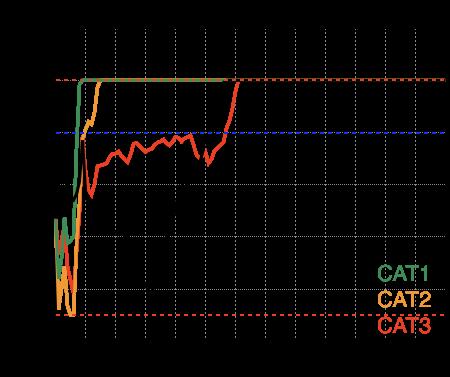
20 The literature on the Catalonian secession is not very helpful because of the large differences in the forecasts of the severity of the post-independence recession. These forecasts range from the 2 percent output loss estimated by Antrás and Ventura (2012) to the 23 percent output loss estimated by Buesa (2012). Moreover, these studies are silent about the short-run dynamics of GDP and, to our knowledge, no-one has studied the consequences of Catalonia s independence for its long-term growth potential. This lack of reliable local studies forced us to look elsewhere. continued study of international secessions came to our rescue. 8 Fortunately, Robert Young s In a 2013 post in the London School of Economics blog, Young (2013) defines a small recession as a drop in output of 3 percent that lasts for 3 years of zero growth, and a large recession as a drop in output of 5 percent that lasts for 4 years of zero growth. He then combines these recessions with two long-run growth rate scenarios: the small recession with a high long-run growth scenario in which the growth rate of the new sovereign state is 1 percent higher than its growth rate before independence, and the large recession with a low long-run growth rate scenario in which this growth rate is only 0.5 percent higher. In this article, we follow Young s suggestions and we simulate four growth rate scenarios which we label sequentially Model Economies CAT0, CAT1, CAT2, and CAT3. Model Economy CAT0, models Catalonia as a Spanish region and, consequently, it replicates Model Economy ESP s exogenous labor productivity growth rate exactly. The endogenous components of the growth processes in this two model economies differ because the age and education distributions of their households and the deterministic components of their labor productivity processes differ as we have discussed above. Model Economy CAT1 replicates Young s small post-independence recession and it models a very successful independent Catalonia. Specifically, output drops by three percent at independence, then it remains constant for the following three years and then it is one percent higher than the growth rate in Model Economy CAT0. Model Economy CAT2 replicates Young s large recession and it models an independent Catalonia that manages to grow more than what it would have grown remaining in Spain, but not by much. Specifically, output drops by 5 percent at independence, then it remains essentially flat for the following four years and then it is 0.5 percent higher than the growth rate in Model Economy CAT0. Finally, Model Economy CAT3 models a failed independence. Specifically, in this model economy output drops by 3 percent at independence, and it remains essentially constant for the following 8 Amongst many other books and research articles, Robert Young is the author of How Do Peaceful Secessions Happen? (Canadian Journal of Political Science 27(04): , December 1994), The Breakup of Czechoslovakia (Research Paper 32, Institute of Intergovernmental Relations, Queen s University, 1994), and The Struggle for Quebec (Montreal and Kingston: McGill-Queens University Press, 1998). 18

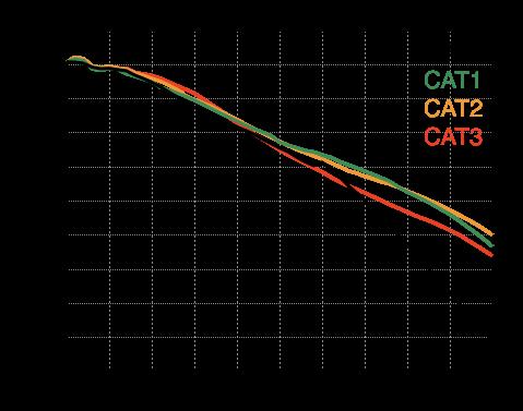
21 three years, but then we assume that Catalonia fails to organize itself better than when it was a region of Spain and that its long-run growth rate replicates the growth rate of Model Economy CAT0. Summarizing, Model Economy CAT1 is the most favorable scenario for independence, and Model Economy CAT3 is the least favorable. We simulate this last scenario to find out whether the educational, productivity, and demographic advantages of Catalonians suffice to compensate for a small post-independence recession without the exogenous boost of an increased productivity growth rate. In Figure 4 we illustrate these growth rate scenarios in our four model economies. The figure shows that replicating Young s scenarios in our model economies is not easy. This is because, in our model economies, the growth rates of output depend on the exogenous labor-augmenting productivity factor, which is easy to determine, but they also depend on the demographic and the educational transitions, whose implications for growth are harder to anticipate and, to complicate matters further, they also depend on the general equilibrium effects that arise from the endogenous responses of the households to every current and future change in every model economy variable. Panel A shows that the post-independence recessions in Model Economies CAT1 and CAT3 are small, short, and very similar to each other, and that the post-independence recession in Model Economy CAT2 is steeper and longer. Model Economies CAT1 and CAT3 return to historical maxima after four years, and Model Economy CAT2 after five years. Panel D shows that it takes until 2034 for Model Economy CAT1 to catch up with Model Economy CAT0 13 years after the independence and that Model Economy CAT2 takes much longer 30 years after the independence. Panels B and E show the partially endogenous and partially exogenous growth rates that deliver these results, and Panels C and F show the exogenous, labor-augmenting productivity processes that we have used to replicate Young s scenarios. In Model Economy CAT1 this process reaches its long-run value in 2041, in Model Economy CAT2 in 2046, and in Model Economy CAT3 in These long-run values are 3.0, 2.5, and 2.0 percent. Figure 4 also illustrates that the economic costs of recessions are large. For instance, in 2023 when the post independence recession is over, output in Model Economy CAT1 is 9.5 percent smaller than in Model Economy CAT0 and the people in this Model Economy have to wait for 20 years, until 2043, before the higher long-run growth rate allows them to recover the lost output. In Model Economy CAT2 these numbers are much worse. In 2024, when the recession ends, in 2024, output is 14.1 percent smaller and the lost output is only recovered in 2069, 49 years after independence. The Fiscal Policy Scenario: The sequences of every exogenous component of fiscal policy are identical in Model Economy ESP and in the four Catalonian model economies with only two exceptions: the consumption tax rates and the sequences of government expenditures. The sequences of consumption tax rates differ because the pension system deficits of our model economies are 19

22 Figure 4: Post-Independence Recessions and Growth Rate Scenarios A: Output Index ( ) B: Output Growth ( , %) C: Productivity Growth ( ,% ) D: Output Index ( ) E: Output Growth ( , %) F: Productivity Growth ( , %) endogenous, and we use consumption taxes to levy the revenues needed to finance pensions when the pension reserve funds run out. 9 The sequences of government expenditures differ by design, because we have decided that their shares of output at market prices should be equal and constant. But the differences between the sequences of consumption rates are only sizeable during the post independence recessions (see Panels L of Figures 5 and Figure 7) and, even though the differences in government expenditures are large, because we keep their ratios to output constant and the differences in output are large, their consequences for the results that we report in this article are also small because transfers other than pensions allow us to clear the government budget every period, and because we have assumed that both government expenditures and transfers other than pensions create no distortions. The Pension System Scenario: The pension systems of Model Economies ESP and CAT0 are identical, and the pension systems of our four Catalonian model economies differ. Their sequences of pension revaluation indexes differ and, therefore, their sequences of minimum and maximum pensions also differ. These differences are endogenous. Their maximum covered earnings sequences also differ, but this time by design, because we have chosen them to be constant fractions of output 9 Model Economy CAT0 inherits the the consumption tax rate sequence form Model Economy ESP, and obviously these sequences are identical but, across the four Catalonian model economies, the sequences of consumption tax rates differ. 20

23 per capita. Every other component of the pension system is identical in Model Economy ESP and in the four Catalonian model economies. The Inflation Rate Scenario: We assume that the inflation rate scenarios are identical in Model Economy ESP and in the four Catalonian model economies. 4 Results In Figures 5, 6, 7, and 8 we illustrate the main findings of our simulations, and in Table 1 we provide a quantitative summary of our findings. As we have already mentioned, every model economy that we study in this article is a growth economy and they all grow for both exogenous and endogenous reasons. The exogenous growth rates that we have assumed for the labor augmenting productivity process account for many of our findings. A quick glance at the time series in the panels of Figures 5, 6, and 7 shows that most of them are exponential curves, and that their main difference is the number of years in which Model Economies CAT1 and CAT2 take to overtake Model Economy CAT0, since Model Economy CAT3 never catches up. Another important reason that accounts for many of our findings is the differences in the Pension Revaluation Indexes (PRI) of our Catalonian model economies. The PRI is designed to keep the pension system in log-run balance, but it is prevented from doing so by its lower and upper bounds. Panel G of Figure 5 and Panel K of Figure 7 show that our four Catalonian model economies eventually reach the PRI s upper bound, and that they remain there for the indefinite future. Model Economy CAT1 reaches the upper bound in 2029, Model Economy CAT2 in 2035, Model Economy CAT0 in 2077, and Model Economy CAT3 in We find that this upper bound of the PRI limits the growth rates of every pension including maximum pensions, well below the exogenous growth rates of these economies. 4.1 Pensions Our simulations of Catalonian independence confirm that, in the short-run, the post-independence recessions will have a negative impact on the sustainability of the pension system of an independent Catalonia. In 2030 the pension system will accumulate debts that range between 8.9 percent of output in Model Economy CAT1 to 11.0 percent of output in model economy CAT2. In the medium-run, after the post-independence recessions are over, the pensions systems of an independent Catalonia recover at various speeds that depend on the long-term growth rates of the model economies. In spite of this, the pension replacement rates decrease continuously in every model economy because the upper bound of the Pension Revaluation Index limits the growth rate of pensions well below the growth rates of output and wages. Finally, we find that, as far as average 21

24 Table 1: Simulation Results Model Rev Exp Def PRF AvP AvA PRI τ c Y A K L C h CEV 2020 ALL CAT CAT CAT CAT CAT CAT CAT CAT CAT CAT CAT CAT CAT , ,837 1,312 1, , CAT , ,377 4,580 6, , CAT ,139 2,293 3, , CAT ,569 1,153 1, , Rev: Pension revenues (%GDP); Exp: Pension expenditures (%GDP); Def: Pension system deficit (%GDP); PRF: Pension reserve fund or pension system debt (%GDP); PRI: Pension Revaluation Index (%); AvP: Average pension (2014=100); AvA: Average retirement age; τ c: Consumption tax rate needed to finance the pension system (%). Y : Output index (2020=100); K: Capital index (2020=100); L: Labor input index (2020=100) h: Total work hours index (2020=100); C: Consumption index (2020=100); CEV : Aggregate Compensating Equivalent Variation (%). 22

25 Figure 5: The Pension System A: Pension System Revenues B: Pension System Payments C: Pension System Budgets D: Average Pension Indexes E: Avg Labor Income F: Pension Replacement Rates G: Average Retirement Ages H: Payroll Tax Exempt Share I: Pension Gini Indexes J: Max and Min Pensions K: Pension Revaluation Indexes L: Consumption Tax Rates 23

26 pensions are concerned, the educational and demographic advantages of Catalonian residents are dwarved by the post-independence recessions. Specifically, in Model Economy CAT3 it takes until 2088 for average pensions to catch up with those of Model Economy CAT0. Pension system revenues: Panel A of Figure 5 shows that pension system revenues as a share of output fall by about one percentage point between 2020 and 2045 and they become relatively constant afterwards. This behavior is noteworthy because it happens in all four or our model economies. Two reasons limit the growth of payroll tax collections and account for this behavior: maximum covered earnings and the delayed retirement of many workers beyond the age in which they they become exempt from paying payroll taxes. As workers become more educated, their wages increase and a larger share of them earn more than the maximum covered earnings, which we have model to remain a constant share of output. In all the three independent Catalonia model economies this happens until about 2045 and in Model Economy CAT0 until about Panel G of Figure 5 shows that something similar happens with the average retirement age. In all four of our model economies it is increasing and, in all four, the average retirement age increases past the age were workers become exempt from paying payroll taxes. 11 Specifically, Panel H of Figure 5 shows that the shares of workers who are exempt from paying payroll taxes increase continuously between 2020 and 2045 or so, from 1 percent to approximately 10 percent and that they become relatively constant in Model Economies CAT1, CAT2, and CAT after 2045, and somewhat decreasing in Model Economy CAT0. Pension system payments: Panel B of Figure 5 shows that the pension system payments to output ratio initially increases because the the post-independence recession and that it decreases afterwards. This happens because output grows at a substantially higher rate than the sum of the growth rates of average pensions and of the number of pensions. This is mostly because the upper bound of the Pension Revaluation Index limits the growth rate of pensions substantially below the long-run growth rate of output. Moreover, Panel B of Figure 5 panel shows that the higher is the long-run growth rate of the model economy the lower is the growth rate of the pension-paymentsto-output ratio. Pension system budgets: Panels A and B of Figure 5 are drawn using the same scale and they show that the changes in the payments of the pension system are substantially larger that the changes in its revenues. Therefore, as Panel C illustrates, the post-independence recession results in pension systems deficits that become pension system surpluses once the recession is over. In Model Economy CAT1 this happens in 2030 and in Model Economy CAT2 in In contrast, the pension system of Model Economy CAT3 is mostly in balance until 2080 or so, because its Pension 10 Specifically, in our model economies, the shares of workers who earn more than the maximum covered earnings increases by about 2 percentage points, from 10.8 percent in 2020 to 12.6, 12.0, 12.0, and 12.1 percent in Between 2014 and 2017, workers who are 65 or older are exempt form paying payroll taxes both in Spain and in our model economies. This tax-exempt age is delayed to 66 between 2018 and 2023, and to 67 from 2024 onwards. 24

27 Revaluation Index (PRI) does not reach its upper bound until then (see Panels K of Figures 5 and 7). This last result confirms that the PRI succeeds in keeping the pension system in balance, as long as its bounds are not binding. In all three independent Catalonia model economies, the pension system surpluses appear in the same year that the PRI reaches its upper bound. Since there is no trade-off that justifies these pension system surpluses, this result shows that the upper bound of the PRI makes little economic sense because it reduces welfare, and because it is inefficient. Average Pensions: Panel D of Figure 5 shows that average pensions are highest in Model Economy CAT1, then in CAT2, and they are similar and lower in Model Economies CAT3 and CAT0. In Model Economy CAT3 average pensions are somewhat lower than in Model Economy CAT0 because of the post-independence recession. This behavior of average pensions is essentially accounted for by the exogenous labor-augmenting productivity growth rates and the PRIs. The productivity growth rates affect average pensions because pension rights track labor income and labor income tracks labor productivity. These results suggest that average pensions will be higher in an independent Catalonia only in as much as it succeeds in growing at a higher rate than Spain. They also suggest that, if Catalonia only manages to grow at a similar rate than Spain, the higher productivity, higher education, and better demographics of Catalonian residents would only make average pensions higher in an independent Catalonia in the very long run, after The time series for Model Economies CAT0 and CAT3 in Panel I of Figure 7 illustrate this finding. Pension Replacement Rates: Panel F of Figure 5 shows that the pension replacement rates are decreasing in every model economy, even though average pensions are increasing. There are two reasons that justify this behavior. First, as we have already mentioned, both the Pension Revaluation Index (PRI) and the maximum pensions limit the growth of pensions. This result is reinforced by the fact that the PRIs reach their upper bound in Model Economies CAT1 and CAT2 relatively early and they remain there indefinitely (see Panel K of Figure 7). Second, the denominator of the pension replacement rate is the average labor income of households in the age group and it grows at a substantially higher rate than average pensions. We have drawn Panels D and E of Figure 5 using the same scale to illustrate this finding. The spikes in the pension replacement rates that occur between 2050 and 2055 result from the reduction in the growth rates of its denominators that take place during those years. Retirement ages: Panel G of Figure 5 shows that average retirement ages first increase between 2020 and about 2060 in all four model economies and then they decrease somewhat. The differences in retirement ages between the three independent Catalonia model economies are always small except in Model Economy CAT1 when households start to retire substantially later from 2070 onwards (see Table 1). The households delay their retirement ages for two reasons: because the 2013 Pension 25

28 System Reform delays the legal retirement ages, and because households become more educated and this makes them retire later. The educational transition ends around 2060 for the cohort and between 2060 and 2070 for the cohort and, consequently, this factor disappears after those years. If we consider the very long run, retirement ages also increase because wages increase and because the upper bound on the Pension Revaluation Indexes makes the pension replacement rates decrease very substantially. These two effects decrease the value of retirement and increase its opportunity cost. In Model Economy CAT1 average retirement ages increase the most because this economy has the lowest pension replacement rate and the highest wage rate. Pension Inequality: Panel I of Figure 5 shows that in all four model economies the Gini Index of pensions decreases between 2020 and In 2020, this index is in every model economy and, in 2070, it ranges between in Model Economy CAT0 and 0.26 in Model Economy CAT2. Once again, this is mostly because of the impact of the Pension Revaluation Indexes (PRI) on the minimum and the maximum pensions. First, the negative PRIs of Model Economies CAT0 and CAT3 reduce the minimum pensions. In response, the households work harder and accumulate more pension rights so that decreasing shares of new retirees collect the minimum pensions in these model economies. Additionally, in Model Economies CAT1 and CAT2, where the PRI is mostly positive, the high labor productivity growth relative to the PRI allows households to accumulate pension rights without having to work longer, and this makes new pensions higher than the minimum pension. Consequently, the share of retirees who receive the minimum retirement pension decreases continuously in all four model economies. 12 Second, after 2045 the share of retirees who receive the maximum retirement pension increases because of the reasons that we have just discussed. 13 Moreover, the lower the accumulated PRI relative to the accumulated growth rate of output, the higher the share of the retirees that collect the maximum pensions. This increases the concentration of pensions at the top of the pension distribution and reduces pension inequality. Because the share of pensioners who collect the maximum pension increases substantially more in Model Economy CAT0 than in the three independent Catalonia model economies, the Gini index of pensions also decreases more in Model Economy CAT0. Finally, as Panel J of Figure 5 illustrates, the range of pensions decreases continuously in all four model economies an this contributes to reduce pension inequality even further. The Pension Revaluation Indexes (PRI): Panel K of Figure 5 shows that in the short run the PRIs are lower in the three independent Catalonia model economies than in Model Economy CAT0. This is because of the post independence recessions. The severity of the recessions and the 12 These shares decrease from 24.9 percent in 2020 to 3.5, 4.4, 4.4, and 4.0 percent in These shares increase from 10.5 percent in 2020 to 40.7, 25.5, 19.9, and 20.6 percent in

29 size of the post recession growth rates determine the duration of the period that it takes for the PRIs of the independent Catalonia model economies to catch up with the PRI of Model Economy CAT0. As Panel K of Figure 7 illustrates, once the PRIs reach their upper bound, they remain there indefinitely. This is because the long term growth rates of all four model economies are substantially higher than the PRIs upper bound, Pension reserve funds: Panel J of Figure 7 illustrates the evolution of the pension reserve funds that result from capitalizing the pension system surpluses at 2 per cent. It shows that it is consistent with the evolution of the corresponding pension system budgets. Model Economy CAT1 has the largest pension system surpluses and it accumulates the most pension reserve fund assets. In contrast, Model Economy CAT3 has the smallest pension system surpluses and, therefore, it only starts accumulating pension reserve assets in the very long run. Consumption tax rates: Finally, Paneld L of Figures 5 and 7 illustrate that consumption tax rates are also consistent with the evolution of the pension system budgets. The consumption tax rate is Model Economy CAT1 returns to its benchmark value of 22.6 in 2030 when the pension system deficit created by the post independence recession disappears, and it remains at that value forever. Model Economies CAT2, CAT3, and CAT0 replicate this behavior in 2036, 2060, and This is because no additional revenues need to be raised to finance the pensions when the pension systems are running surpluses and, consequently, the consumption tax rates remain unchanged. 4.2 Macroeconomic Variables The exogenous growth of labor market productivity generates a sustained growth of output per capita in our four model economies. Additionally, in all of them, the increased education of the households increases the efficient labor input and the reductions in pension replacement rates encourage savings. These two factors contribute to increase the size of the capital stocks and compound the growth rate of output per capita. Output: Panel A of Figure 6 shows that output in Model Economy CAT1 catches up with output in Model Economy CAT0 in 2034, 13 years after independence, and that the output lost during the post-independence recession is recovered in 2043, 22 years after independence. In Model Economy CAT2 the output catch-up occurs in 2051, 30 years after independence and the output lost is recovered in 2069, 48 years after independence. These results are similar to those obtained by Young (2013). As expected, output in Model Economy CAT3 never catches up with output in Model Economy CAT0 because their long term growth rates are identical. Capital and labor inputs: Panels B and C of Figure 6 show that the total labor input, which includes the labor-augmenting productivity factor, grows by more than the capital input, but not by much. Obviously the growth rate of output falls in between the growth rates of the two inputs. The capital 27

30 Figure 6: Macroeconomic Variables A: Output B: Capital Input C: Total Labor Input a D: Labor Productivity Factor E: Efficient Labor Input b F: Labor Hours G: Consumption H: Investment I: Government Expenditures J: Earnings Gini Indexes K: Income Gini Indexes L: Wealth Gini Indexes These statistics are expressed as a percentage of output. a This measure of the labor input includes the exogenous, labour-augmenting productivity factor, A. b This measure of the labor input does not include the exogenous, labour-augmenting productivity factor, A. 28

31 stock increases because labor earnings increase due to the increase in labor productivity, because the shares of more educated people increase, because the reductions in pension replacement rates, and because the shares of older people increase. Note that the increases in the shares of more educated people and older people are the same in all four of our model economies. Productivity, efficient labor input, and hours: Panels D, E, and F of Figure 6 show that most of the growth in the total labour input is accounted for by the growth of the exogenous, labor-augmenting productivity factor. In contrast the efficient labor input increases by little and labor hours remain essentially flat. Those panels also show that the differences in the efficient labor input and in labor hours between our four model economies are small. The efficient labor input increases until around 2050 because of the educational transition. By this year, it becomes relatively constant because the educational transition of the working-age population is coming to its end. Additionally, the ageing of the Catalonian population reduces the number of workers and these two effects approximately cancel each other out after 2050 or so. Finally, the post-independence recessions, result in a small dip in labor hours. After the recessions are over, hours become relatively constant because the income and substitution effects that result from the increased wages essentially cancel each other out. Consumption, investment, and government expenditures: Panels G, H, and I of Figure 6 show that the growth rates of consumption, investment, and government expenditures are similar and that the post-independence recession effects are most noticeable in the investment series. Those panels confirm that exogenous long-run growth rates account for most of the consequences of independence and more than compensate for its short-term effects, and endogenous factors. Earnings, income, and wealth inequality: Panels J, K, and L of Figure 6 show that earnings, income and wealth inequality dip during the post-independence recessions and that they increase somewhat in the long run. 4.3 The Long Run To understand the welfare findings that we discuss below, we must realize that they depend crucially on the very long-run consequences of the independence of Catalonia. In 2021, which is our assumed independence date, the youngest households in our model economies are 20 years old. They were born in 2001 and they may live up to 100, that is until But in our welfare calculations we also take into account the welfare of the households who enter the economy between 2021 and The youngest of these households were born in 2050 and they may live until Therefore the time period that we consider in this section and in the next section is the years between 2020 and This implies that the households whose decisions we are studying were born between 1920 and

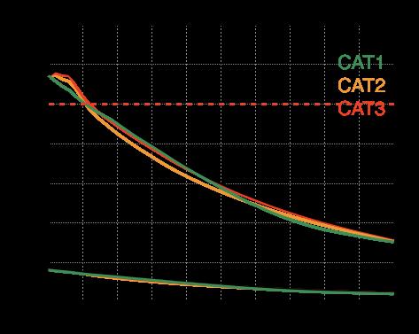
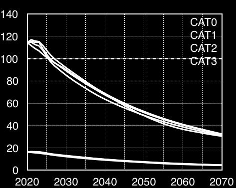
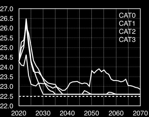
32 Figure 7: The Long Run A: Output B: Capital C: Total Labor Input D: Labor Productivity Factor E: Efficient Labor Input F: Labor Hours G: Consumption H: Labor Income I: Pensions J: Pension Reserve Funds K: Pension Revaluation Indexes L: Consumption Tax Rates 30

33 In Figure 7 we plot the main time series that describe the long-run behaviour of our four model economies. The panels in this figure tell pretty much the same story as those in Figure 6. That is, that the short-term losses in consumption, wages, and pensions brought about by the postindependence recessions become long-term gains in Model Economies CAT1 and CAT2, and that Model Economy CAT3 never catches up with Model Economy CAT0. Moreover, the time that it takes before the catch-ups take place is increasing with the severity of the recessions. For instance, in Model Economy CAT1 aggregate consumption catches up with Model Economy CAT0 in 2030, and in Model Economy CAT2 this happens in The catch-up dates for pensions are 2034 and 2041 and, for labor income, 2036 and Perhaps the most interesting finding of Figure 7 is that average pensions are the only variable for which Model Economy CAT3 catches up with the corresponding variable of Model Economy CAT0, and that this happens in 2088 (see Panel I). This is because of the demographic and educational advantages of Catalonian residents over the residents in the rest of Spain. These advantages result in a higher PRIs and in higher pensions in all the Catalonian economies. In Model Economy CAT3, this happens the very long run once the effects of the post-independence recessions are well over. In contrast, Panel H of Figure 7 shows that average labor income is lower in Model Economy CAT3 than in Model Economy CAT0 for the entire period that we consider. This because the exogenous productivity growth rates and the demographic and educational transitions in these two model economies are identical, and this implies that the long-term growth rates cannot compensate the reductions in labor income that result from the post-independence recessions. Quantitatively, we find that the lower long-run growth rate of labor income more than compensates for the higher long-run growth rate of pensions and that, therefore, consumption in Model Economy CAT3 is lower than in Model Economy CAT0 during the entire period that we consider (compare Panels G, H, and I of Figure 7). This result implies that the higher consumption of Model Economy CAT3 retirees is not enough to compensate for the lower consumption of its workers. 4.4 Welfare In Figure 8 we quantify the consequences of independence for the welfare of Catalonian households. In Panel A of that figure we plot the aggregate welfare consequences and in Panel B the welfare consequences organized by the year of birth of the households. The sample that we consider in both panels is made up of the households who were born between 1921 and 2050, the time period that we consider to compute the welfare costs is between 2021 and Aggregate welfare consequences: Panel A of Figure 8 confirms the intuition that the consequences of independence for Catalonian residents will depend crucially on the long term growth rate of the 14 The graphs in Figure 8 start in 2020 and 1920 to improve the labelling of the horizontal axis. 31

34 new republic. It also shows that the demographic, educational, and productivity advantages of Catalonian residents, when compared with those of the rest of Spain, are not enough to ensure a more prosperous economic future for Catalonians. Specifically, independence results in increasing aggregate welfare gains in Model Economies CAT1 and CAT2 and in increasing aggregate welfare losses in Model Economy CAT3 for the entire period that we consider. In 2021 these welfare gains and losses are 17.2, 3.4, and 6.4 percent of aggregate consumption and, in 2070, they are 75.5, 26.3 and 7.8 percent of aggregate consumption. Welfare consequences by year of birth: To discuss the welfare consequences by year of birth, we split our sample into into two sub-samples: one made up by the households who were born between 1921 and 2001, and another one made by the households who were born between 2002 and The households in the first sub-sample entered our model economies before the independence took place and, presumably, a majority of them voted in its favor. The households in the second sub-sample entered our model economies after the independence took place, and enjoyed or suffered the consequences of a political decision in which they did not participate. (a) The welfare of the households who had entered the economy before independence. We find that independence imposes a welfare cost on the households who were born before 1937 in Model Economy CAT1, on those who were born before 1952 in Model Economy CAT2, and on every household who was born before independence in Model Economy CAT3. Those households were 84, 69, and 20 years old in 2021, at the time of independence. Figure 8: Welfare (CEV, %) A: Aggregate Welfare Costs B: Wefare Costs by Year of Birth In Model Economy CAT1, the households that were born between 1921 and 1936 that is, those who were 85 or older old at the time of the independence in 2021 loose with the independence because of the short-run increase in consumption taxes and the short-run reduction in pensions. But the households born after 1936 that is, those who were younger than 85 in 2021 are better off in this model economy because their consumption taxes are lower and their wages and retirement 32