Three Papers on the Black-White Mobility Gap in the United States. Liana E. Fox

Transcription

1 Three Papers on the Black-White Mobility Gap in the United States Liana E. Fox Submitted in partial fulfillment of the requirements for the degree of Doctor of Philosophy under the Executive Committee of the Graduate School of Arts and Sciences COLUMBIA UNIVERSITY 2013

2 2013 Liana E. Fox All rights reserved

3 ABSTRACT Three Papers on the Black-White Mobility Gap in the United States Liana E. Fox Paper 1/Chapter 2: Missing at Random? An Analysis of the Effect of Sample Selection on Intergenerational Earnings Elasticities by Race Utilizing the Panel Study of Income Dynamics, I assess the effect of sample selection bias on estimates of intergenerational earnings elasticities for white and black father-son pairs, regressing log child earnings on log parent earnings. Estimating four increasingly less selected models, I assess the robustness of estimates to alternative methods of handling sons who are missing data due to periods of unemployment or part-time employment. The results indicate that the assumption of exogenous selection into full-time employment significantly biases the estimates for blacks, although it does not have a large impact on estimates for whites. As a consequence, selection bias will understate the magnitude of the black-white mobility gap. The results also indicate that two methods substantially mitigate this selection bias: having a long panel, or imputing data in a short panel. Paper 2/Chapter 3: Measuring the Black-White Mobility Gap: A Comparison of Datasets and Methods Chapter 3 utilizes both the National Longitudinal Survey of Youth (NLSY) and the Panel Study of Income Dynamics (PSID) to analyze the magnitude and nature of black-white gaps in intergenerational earnings and income mobility in the United States. This chapter finds that relying on different datasets or measures will lead to different conclusions about the relative magnitudes of black versus white elasticities and correlations, but using directional mobility matrices consistently reveals a sizable mobility gap between black and white families, with low-

4 income black families disproportionately trapped at the bottom of the income distribution and more advantaged black children more likely to lose that advantage in adulthood than similarly situated white children. I find the family income analyses to be most consistent and estimate the upward mobility gap as between 19.1 and 20.3 percentage points and the downward gap between and Additionally, I find that racial disparities are much greater among sons than daughters and that incarceration and being raised in a female-headed household have much larger impacts on the mobility prospects of blacks than whites. Paper 3/Chapter 4: Can Parental Wealth Explain the Black-White Mobility Gap? Utilizing longitudinal data from the Panel Study of Income Dynamics (PSID), this chapter examines the relationship between parental wealth and intergenerational income mobility for black and white families. I find that total parental wealth promotes upward mobility for lowincome white families, but does not protect against downward mobility for white families from the top half of the income distribution. Conversely, I find that total parental wealth does not assist low-income black families while home ownership may have negative associations with the likelihood of upward mobility for these families. However, for black families from the top half of the income distribution home equity is protective against downward mobility suggesting a heterogeneous relationship between home ownership and mobility for black families.

5 TABLE OF CONTENTS LIST OF TABLES AND FIGURES... ii ACKNOWLEDGMENTS... vi DEDICATION... viii CHAPTER 1: INTRODUCTION... 1 CHAPTER 2: MISSING AT RANDOM? AN ANALYSIS OF THE EFFECT OF SAMPLE SELECTION ON INTERGENERATIONAL EARNINGS ELASTICITIES BY RACE... 3 CHAPTER 3: MEASURING THE BLACK-WHITE MOBILITY GAP: A COMPARISON OF DATASETS AND METHODS CHAPTER 4: CAN PARENTAL WEALTH EXPLAIN THE BLACK-WHITE MOBILITY GAP? CHAPTER 5: CONCLUSION i

6 LIST OF TABLES AND FIGURES Table 2.1: Intergenerational Elasticities, by Model Specification and Race Table 2.2: First-Stage Imputed Earnings Results, Table 2.3: Comparison of Intergenerational Elasticities by Actual vs. Imputed Earnings and Race Figure 2.1.A: Only FT (N=444) 25 Figure 2.1.B: Lower-Bound (N=757) Figure 2.1.C: Upper-Bound (N=757) Appendix Table 2.1: Average Earnings, by model specification and race 26 Table 3.1: Descriptive Statistics for NLSY v PSID Samples Table 3.2: Intergenerational Elasticities and Correlations PSID v NLSY 55 Table 3.3: Likelihood of Upward and Downward Mobility by Race, NLSY and PSID...56 Appendix Table 3.1: Intergenerational Elasticities and Correlations by Incarceration History, Overall...57 Appendix Table 3.2: Intergenerational Elasticities and Correlations by Incarceration History, White, non-hispanic Families...58 Appendix Table 3.3: Intergenerational Elasticities and Correlations by Incarceration History, Black, non-hispanic Families...59 Appendix Table 3.4: Intergenerational Elasticities and Correlations by Family Structure, Overall...60 Appendix Table 3.5: Intergenerational Elasticities and Correlations by Family Structure, White, non-hispanic Families...61 Appendix Table 3.6: Intergenerational Elasticities and Correlations by Family Structure, Black, non-hispanic Families...62 Appendix Table 3.7: Likelihood of Upward and Downward Mobility by Race for Never- Incarcerated Population, NLSY and PSID 63 Appendix Table 3.8: NLSY Family Income-Family Income Mobility Matrices by Race (Sons & Daughters). 64 ii

7 Appendix Table 3.9: NLSY Family Income-Family Income Mobility Matrices by Race (Sons). 65 Appendix Table 3.10: NLSY Family Income-Family Income Mobility Matrices by Race (Daughters) Appendix Table 3.11: NLSY Family Income-Child Earnings Mobility Matrices by Race (Sons & Daughters) Appendix Table 3.12: NLSY Family Income- Child Earnings Mobility Matrices by Race (Sons). 68 Appendix Table 3.13: NLSY Family Income- Child Earnings Mobility Matrices by Race (Daughters) Appendix Table 3.14: PSID #3 Family Income-Family Income Mobility Matrices by Race (Sons & Daughters) Appendix Table 3.15: PSID #3 Family Income-Family Income Mobility Matrices by Race (Sons). 71 Appendix Table 3.16: PSID #3 Family Income-Family Income Mobility Matrices by Race (Daughters) Appendix Table 3.17: PSID #3 Family Income-Child Earnings Mobility Matrices by Race (Sons & Daughters) Appendix Table 3.18: PSID #3 Family Income-Child Earnings Mobility Matrices by Race (Sons). 74 Appendix Table 3.19: PSID #3 Family Income-Child Earnings Mobility Matrices by Race (Daughters) Appendix Table 3.20: PSID #3 Father Earnings-Child Earnings Mobility Matrices by Race (Sons & Daughters) Appendix Table 3.21: PSID #3 Father Earnings-Child Earnings Mobility Matrices by Race (Sons). 77 Appendix Table 3.22: PSID #3 Father Earnings-Child Earnings Mobility Matrices by Race (Daughters) Figure 4.1: Median Family Net Worth, (in 2009$)..99 Figure 4.2: Median Family Net Worth Excluding Home Equity, (in 2009$)...99 iii

8 Figure 4.3: Distribution of White Families by Net Worth, Figure 4.4: Distribution of Black Families by Net Worth, Figure 4.5: Median Net Worth by Race and Head Education, Figure 4.6: Distribution of Parent Generation Figure 4.7: Distribution of Child Generation Table 4.1: Demographic Characteristics of Sample by Race and Parental Ranking..103 Table 4.2: Parental Wealth Holdings by Asset Type and Race, (2009$)..104 Table 4.3a: Likelihood of Upward Mobility by Race Figure 4.8: Upward Mobility by Race, Parent Rank<= Figure 4.9: W-B Upward Mobility Gap Table 4.3b: Likelihood of Downward Mobility by Race..107 Figure 4.10: Downward Mobility by Race, Parent Rank> Figure 4.11: W-B Downward Mobility Gap.108 Table 4.4a: Likelihood of Upward Mobility from Bottom 20%, Conditional on Parental Wealth Attributes Table 4.4b: Likelihood of Downward Mobility from Top 50%, Conditional on Parental Wealth Attributes Table 4.5: Likelihood of Mobility by Asset Values and Race..110 Table 4.6: Real Home Equity (low income home owners in 1984)..111 Table 4.7: Decomposition of the Effects of Wealth on White-Black Upward Mobility Gap Appendix Figure 4.1: Percentiles of Net Worth for White Families, Appendix Figure 4.2: Percentiles of Net Worth for Black Families, Appendix Table 4.1a: Likelihood of Upward Mobility by Race Adjusted by Family Size 114 Appendix Table 4.1b: Likelihood of Downward Mobility by Race.114 Appendix Table 4.2a: Likelihood of Upward Mobility by Race Adjusted by Family Size 115 Appendix Table 4.2b: Likelihood of Downward Mobility by Race.115 iv

9 Appendix Table 4.3a: Likelihood of Upward Mobility by Race Adjusted by Family Size 116 Appendix Table 4.3b: Likelihood of Downward Mobility by Race.116 Appendix Table 4.4: Decomposition of Wealth on Upward Mobility.117 v

10 ACKNOWLEDGMENTS Over the past four and a half years I have received support and encouragement from a great number of individuals. First and foremost I would like to express my deepest gratitude to my advisor, Jane Waldfogel, for her never-ending encouragement, guidance and providing me with an excellent atmosphere for doing research. I owe sincere and earnest thankfulness to my sponsor, Irwin Garfinkel, who has continually challenged and enriched my understanding of social welfare policy. I am also very thankful to the rest of my dissertation committee of Ronald Mincy, Seymour Spilerman and Judith Scott-Clayton for providing me with advice and encouragement through coursework and individual meetings as my interests have developed. I would like to express my gratitude to my classmates Nathan Hutto and Leyla Karimli for their generous friendships and solidarity. Thanks to Natasha Pilkauskas and Afshin Zilanawala for answering my streams of questions and providing much needed breaks throughout this process. I would also like to thank my previous advisors and mentors: Kate Bronfenbrenner who helped channel my social justice consciousness, Stephanie Luce who helped me gain a deeper understanding of the power of empirical research, Mark Brenner who patiently spent hours teaching me SAS, and Michael Ettlinger who introduced me to the world of policy analysis. Finally, I would like to thank my family, both immediate and extended, for their encouragement and support. I thank my daughter Hazel for teaching me a new level of time management and multitasking. Not the least, I appreciate the personal and financial sacrifices made by my husband Chris which allowed me to pursue this degree. Thank you for being my teammate. vi

11 This research was supported by the Columbia Population Research Center (award number R24HD from the Eunice Kennedy Shriver National Institute of Child Health & Human Development) for travel support to present Chapters 2 and 4 at the Population Association of America s Annual Meetings. Research for Chapter 4 was also supported by a grant from the Pew Charitable Trusts and Charles Stewart Mott Foundations. Opinions reflect those of the author and do not necessarily reflect those of the granting agencies. vii

12 DEDICATION To my family generations past and future. viii

13 1 CHAPTER 1: INTRODUCTION The United States is often described as the land of opportunity. However, with the dramatic increase in income inequality since the 1970s, the equality of this opportunity has been called into question. As a society, we are willing to tolerate inequality as long as there is fairness and opportunity for all individuals to succeed, regardless of family background. However, recent analyses (Hertz 2007; Isaacs 2008) find that opportunity may not apply equally to all citizens. While the black-white male wage gap has closed considerably since passage of the Civil Rights Act of 1964, black families are more likely to remain poor and experience relative (and often absolute) declines in income position from one generation to the next compared with white families. From a social welfare perspective, this means that an extra dollar of income does not guarantee the same level of long-run economic success for black families as white families. Research focusing on black-white economic disparities has found a narrowing of the male wage gap from 50% in 1967 to 27% in 1998 (Couch and Daly 2002), while the family income gap has closed considerably less, with median black family income comprising 59% of the median white family income in 1967 and 62% in 2007 (Mishel, Bernstein and Shierholz 2009). These comparisons highlight the importance of examining both individual earnings and family income to get a complete portrait of relative economic well-being and opportunity. One measure of opportunity in society is intergenerational mobility, which can be measured by examining the relationship between children s income or earnings with respect to the same measure for their parents. This relationship can be quantified by estimating the elasticity or correlation or by predicting the likelihood of directional mobility between two generations. Higher elasticities indicate greater similarity between outcomes for children and parents and therefore lower mobility. While conceptually the most complete measure of

14 2 intergenerational transmission of economic well-being would be the comparison of parental family income to child family income, it also conflates trends and disparities in employment and family structure. However, examining only earnings results in a selected sample that may not be representative of the total population. Therefore, deciding when to examine intergenerational persistence in family income versus individual earnings represents a tradeoff between a more inclusive measure and population and a better-defined mechanism structure. This dissertation explores several methodological issues in estimating the magnitude of these disparities, as well as examines the role of wealth in explaining the black-white mobility gap. Chapter 2 utilizes the Panel Study of Income Dynamics (PSID) to provide new estimates of intergenerational earnings elasticities for white and black father-son pairs estimated using the traditional methodology of regressing log child earnings on log parent earnings. This chapter pays special attention to the impact of sample selection (i.e. excluding unemployed or part-time employed sons from the sample) on intergenerational mobility estimates. I generate predicted estimates of son s potential earnings (as actual earnings have been censored due to either unemployment or underemployment) and then perform a bounding exercise to examine the range of estimates. Chapter 3 expands on Chapter 2 by comprehensively examining family income mobility in addition to earnings mobility. The more inclusive measure of family income extends the previous analysis of father-son earnings to include all sources of economic well-being and also allows for the examination of individuals from otherwise excluded family structures such as female-headed households. This chapter utilizes both the National Longitudinal Survey of Youth (NLSY) and the Panel Study on Income Dynamics (PSID) datasets as well as multiple methods of estimating intergenerational mobility (elasticities, correlations and directional rank matrices)

15 3 to quantify the magnitude and nature of the black-white family income mobility gap in the United States. It also tests the sensitivity of results to incarceration and family structure. Chapter 4 builds off of methodological advances discussed in the previous two chapters in an effort to explain the mobility gap by examining the relationship between parental wealth and intergenerational income mobility for black and white families. Utilizing the PSID Wealth Supplements, I estimate how parental wealth impacts children s directional income mobility for black and white families and explore differences in this impact by asset type. I also perform a decomposition analysis to investigate the role of wealth/capital accumulation in explaining the economic mobility gap. Finally, Chapter 5 provides a summary of the main results from Chapters 2-4 and discusses implications for policy and social work practice. While the individual chapters cover slightly different years and cohorts, with parental resources measured in in Chapter 2, in Chapter 3 and in Chapter 4, and child resources measured in in each chapter, an attempt is made to compare results across chapters. Areas of future research are also highlighted. REFERENCES Couch, K. and M. C. Daly. (2002). Black-white wage inequality in the 1990s: A decade of progress. Economic Inquiry. 40(1): Hertz, T. (2007). Trends in the intergenerational elasticity of family income in the United States. Industrial Relations. 46(1): Isaacs, J.B. (2008). Economic Mobility of Black and White Families. In Isaacs, J.B. Sawhill, I. and Haskins, R. Getting ahead or losing ground: economic mobility in America. (Washington D.C.: Brookings Institute). pp Mishel, L., J. Bernstein and H. Shierholz. (2009). The State of Working America, 2008/2009. Ithaca, NY: ILR Press, an imprint of Cornell University Press.

16 4 CHAPTER 2: MISSING AT RANDOM? AN ANALYSIS OF THE EFFECT OF SAMPLE SELECTION ON INTERGENERATIONAL EARNINGS ELASTICITIES BY RACE INTRODUCTION Intergenerational mobility is an important measure of social equality and opportunity in a country. Higher mobility signals more potential for individuals to prosper or fail based on individual effort or attributes, while lower mobility signals a system where status is primarily based on family background. Economists and sociologists have been attempting to measure intergenerational mobility for decades, but new methods continue to challenge previous findings (Solon 1999; Black & Devereux 2010). Previous research has highlighted the importance of using permanent income measures rather than single-year income measures (Grawe 2006; Haider & Solon 2006). Similarly, due to life-cycle variation in income, the age at which income is observed matters quite a bit, and ideally should be measured from both generations while they are in their 30s-40s (Solon 1999; Black & Devereux 2010) and age-adjusted to account for age differences within a sample (Solon 1992; Bratberg et al 2007). Additionally, more recent work has focused on non-linearities in mobility, with both the lowest and highest income families experiencing a greater deal of stickiness than do middle income families (Hertz 2005; Grawe 2004; Eide & Showalter 1999). While all these potential sources of bias have been corrected for in recent research, there still exists one potentially serious concern: sample selection bias. Typically, intergenerational mobility is measured by estimating the elasticity between parents income or earnings and the same measure for their children. Higher elasticities (i.e. closer to 1) indicate greater reliance on parents income and therefore lower mobility (the direction of mobility upward or downward cannot be discerned from elasticity measures). When calculating the

17 5 intergenerational elasticity it is common to exclude unemployed and part-time employed children (or individuals who report no income or earnings) from the sample with the assumption of exogenous selection into full-time employment. However, evidence suggests that sons from lower income families may have a weaker attachment to the labor force and therefore lower mobility, so excluding individuals with perhaps the highest elasticities introduces a downward bias to the current intergenerational elasticity estimates. A few papers have examined selection bias in the intergenerational mobility literature and found it to be a problem (Couch & Lillard 1998; Minicozzi 2003; Francesconi & Nicoletti 2006). However, this literature has not examined the effect of selection bias on estimates of how mobility differs by race. This is a potentially serious omission given that the extent of bias associated with missing employment data is likely to be much more severe for blacks than for whites, given their lower adult employment rates. This chapter therefore provides new estimates of intergenerational elasticities for blacks and whites explicitly taking into account the effect of selection bias. To that end, I examine the impact of four alternative approaches to missing data on sons earnings. The first model follows the standard assumption of exogenous selection into full-time employment, restricting the sample to sons who were employed full-time at age 35/36 and 37/38. The second model reduces missing data by imputing a predicted value of sons earnings for individuals with earnings censored by part-time employment or unemployment. The third model also reduces missing data by utilizing upper and lower bounds on sons earnings that have been censored by part-time employment or unemployment to estimate the range of potential elasticities. Finally, the fourth model is the most inclusive, allowing information on sons earnings from full-time employment to be drawn from 20 years of data (from son s age 35-55), a specification that would only

18 6 exclude individuals who dropped out of the PSID or who were consistently unemployed or parttime employed for their entire prime-age working careers. BACKGROUND In attempting to explain the differences in intergenerational mobility estimates in the literature, several papers have examined the impact of sample selection bias. First, Couch and Lillard (1998) found that intergenerational correlations are very sensitive to selection rules. They found that a more restrictive sample, which was often more homogenous, led to higher intergenerational income correlations. Specifically the authors warn against excluding estimates of low-earnings (even if due to part-time employment or unemployment); stating that such exclusions should only be done if one is trying to explicitly identify a sub-population, not examine overall mobility rates. However, in 2003, Minicozzi found the opposite result excluding part-time and unemployed workers biased the intergenerational elasticities downward. Minicozzi found that differential treatment of part-time employed workers accounts for some of the variation in estimates across current studies. While the exact reasons for the disparities in findings between Couch and Lillard and Minicozzi are not readily apparent, Minicozzi had a larger sample size and focused on sons aged 27-29, while Couch and Lillard had a wider age range (22-30). Studies that estimate elasticities at younger ages tend to produce smaller estimates (Solon 1999), but that would suggest that Couch and Lillard s estimates should be lower than Minicozzi s which was not the case. In 2006, Francesconi and Nicoletti set aside earlier findings on sample selection and focused on non-labor market selection processes such as non-ignorable attrition and short panels. They found evidence of co-residence bias, which means that children who co-reside with

19 7 their parents at late ages will have better measures of initial status due to more years of measured parental income. The authors find evidence of a downward bias in intergenerational elasticities, especially at the ends of the occupational prestige distribution (used instead of earnings/income to avoid labor market selection issues). This bias is especially problematic in short panels. Taken together, these three papers highlight the importance of sample selection, although the ultimate direction of bias is unclear. DATA For this analysis, I use the Panel Study on Income Dynamics (PSID), which is a longitudinal survey that follows individuals and their offspring from 1968 to present. The survey was conducted annually from and biannually since then, with the most recent data covering The PSID includes rich data on labor earnings, hours worked, employment status and family relationships. Using this data it is possible to identify individuals whose earnings have been censored by working part-time or part-year, but unfortunately it is not possible to tell whether individuals are voluntarily choosing to work part-time, or whether this type of employment is due to economic conditions restricting their opportunities. Sample Restrictions As one of the main goals of this analysis is to examine the effect of sample selection on intergenerational elasticity measures, I am very deliberate about selecting my own sample. Since the issue of selection becomes much less clear when thinking about women opting out of the labor force to raise children, I focus my analysis on the relationship between sons and their fathers. 1 As a very high percent of prime-age men work full-time, it is not a stretch to assume 1 Implicit in this framework is that I am only looking at sons raised in male-headed families since I am looking at the relationship between father and son earnings. I choose this restriction so as to focus on issues related to intergenerational earnings transmissions and not to confuse the issue of family structure. A preliminary analysis suggests that individuals raised in female-headed families have considerably lower income elasticities (i.e. sons

20 8 that most prime-age men would work full-time if they had the opportunity, which theoretically allows the assumption of exogenous selection into full-time employment to have some validity. My overall sample is restricted to white and black father-son pairs in the PSID with at least three years of valid father earnings while the son was living at home under 21 years old and the father was between age As a result of these restrictions, the father cohort was born between and the son cohort was born between Further restrictions for each model are detailed below. Earnings in the PSID include the individual s annual earnings from labor including salaries, wages, bonuses, overtime, and commissions. For this analysis, earnings are first adjusted to 2006 dollars using the CPI-U, logged and then averaged for all available years. Father s earnings are only included for years when the son lived at home and was age 21 or below and the father was between 35 and 55 years old. Sons earnings are included for years when the son lived outside of his parents home and was employed full-time (>2,000 hours/year). METHODS Following the standard intergenerational mobility methodology (Black & Devereux 2010), I calculate the intergenerational earnings elasticity by regressing the log of permanent child earnings on the log of permanent parent earnings: ( ) (1) earnings are much less related to parents earnings) than individuals raised in a two-parent family (0.11 vs elasticity). This assumption is especially important when looking at families by race, as a very rough examination of a single year of PSID data shows that 37% of black sons lived in a female-headed family compared with 11% of white sons. However, family structure is volatile, so many of these individuals are included in the final sample in years when their father (or other cohabiting adult male) is present. Chapter 3 explores relaxing this restriction. 2 Findings are robust to choice of restriction on fathers ages, whether they are restricted to age or Age range of was used in this analysis to be consistent with recommendations from Haider and Solon (2006) and the age restriction used in Model 4.

21 9 Consistent with current methodology (Black & Devereux 2010), I estimate Equation 1 by first subtracting the mean value of log earnings from each observation to suppress the constant term (Equation 1a) and then age-adjust son and parent earnings to account for life-cycle variation in earnings (Equations 1b & 1c). 3 ( ) ( ) ( ) (1a) To age-adjust earnings, I follow previous research (Bratberg et al 2007) and regress log earnings on age and age-squared and use the residual in the final estimation equation: ( ) ( ) (1b) ( ) ( ) (1c) This results in the following simplified equation: (2) where is the intergenerational earnings elasticity, lower-case is the age-adjusted, demeaned value of log earnings and is the error term. The interpretation of is that the closer it is to 1, the less mobility in society, as a large percent of variation in a son s earnings comes from his father s earnings, while the closer is to 0, the greater the mobility. 4 This is the method used for calculating intergenerational elasticities in all of my models, although the procedure for estimating and selecting sons into the sample varies from model to model. For each model I estimate an overall elasticity, a white elasticity and a black elasticity. I start from the most restrictive model and expand out, investigating alternative methodologies for estimating permanent child earnings which allow for the inclusion of a greater 3 Mean values of both son and father earnings can be found in Appendix Table There is a great deal of debate on the optimal level of mobility in society (see Bowles, Gintis & Osborne Groves 2005).

22 10 number of father-son pairs into the sample, which should therefore allow for greater representativeness and generalizability of results. Model 1: Exogenous selection into full-time employment In my first model, I restrict the sample to sons who were employed full-time at both age 35/36 and age 37/38 (N=444). This model best estimates the current methodology in the literature, which assumes that sons are exogenously selected into full-time employment. This is the most restrictive model as no information from sons who are employed part-time or unemployed is included in this estimation of intergenerational elasticity. Additionally, individuals with missing earnings data during either of these two time periods are excluded. In this specification I am drawing on 2 years of sons earnings and an average of 9.7 years of fathers earnings information. Average earnings can be found in Appendix Table 2.1 for each model specification both overall and by race. Model 2: Imputed earnings at age 35/36 and 37/38 for part-time/unemployed sons To examine the role of exogenous selection, I estimate an imputed value of son s potential earnings as a proxy for actual labor earnings. 5 Potential earnings at age 35/36 and 37/38 are estimated from the average earnings from full-time employment while age and age as well as a range of demographic characteristics. In my imputation the first-stage equation is: (3) 5 Alternatively, in lieu of this imputation procedure, I could have used earnings from sons in their twenties and used an adjustment factor to scale up these values, but I was hesitant to use such an adjustment factor due to differences in life-cycle growth of wages. According to Haider and Solon (2006), using earnings from an individual in their twenties causes a large attenuation bias, but the bias is small if earnings are measured between the early thirties and the mid-forties. Additionally, Haider and Solon found that individuals with the greatest potential lifetime earnings often have lower earnings than other individuals early on in their careers as this time is often spent in education or taking risks (i.e. starting a business) with larger potential payouts in the future. To avoid this life-cycle bias, I chose to impute earnings values based on average actual earnings at both younger and older ages, as well as other human capital components such as education and marital status.

23 11 where is average earnings from full-time employment at age and age and is a vector of individual characteristics (educational attainment, race, age, age-squared, marital status, and state of residence). The results from this first-stage equation are displayed in Table 2.2. From this equation, I then generate predicted values of for all sons and plug those values into equation 2. Therefore, my second-stage equation is: (4) where is the intergenerational earnings elasticity adjusted for selection with the same interpretation as the earlier elasticity. For consistency, all sons are given imputed values for even if they had valid earnings information for those years. An examination of this imputation process can be found in Table 2.3, which compares imputed earnings to actual earnings. By imputing values of sons earnings for unemployed and part-time employed sons, the sample size for this model increases to 757. In this specification I utilize an average of 4.5 years of sons earnings and an average of 9.4 years of fathers earnings information (see Appendix Table 2.1 for average values of earnings). Model 3: Estimation of upper and lower bounds Subsequent to the imputation regressions, I follow Minicozzi (2003) to estimate upper and lower bounds of sons earnings to verify the accuracy of the imputation procedure and estimate the range of potential elasticities. To calculate the lower-bound, I use the earnings value equal to the maximum of either the lowest reported logged child income from full-time employment for the sample of sons who worked full-time at both age 35/36 and 37/38, which is 7.56 or the individual s actual average log reported earnings from age 35/36 and 37/38. Actual earnings could be from either part-time employment or partial-year employment stemming from

24 12 unemployment. 6 This procedure is consistent with Minicozzi s modified lower-bounds estimate: (5) For the vast majority of individuals, their own averaged actual earnings from age 35/36 and 37/38 are greater than 7.56 (unlogged 7.56 is equal to less than $2,000/year). In fact, the lower bound estimate of 7.56 is only binding for 18 of the 313 lower-bound earnings estimates for sons. For the upper-bound, I loosely follow Minicozzi s modified upper-bound estimate, but instead of dividing my sample into 10 different categories with varying upper-bound estimates I simply divide my sample into two groups: Group A who had one year of full time employment at age 35/36 or 37/38 and Group B who was not full-time employed at either 35/36 or 37/38. The upper bound for individuals in Group A is simply the single year of earnings from full-time employment at either 35/36 or 37/38. The upper-bound for individuals in Group B is the maximum single year of earnings received from any type of employment (including part-time and part-year employment) from age (6) (7) Figures 1A-C show scatter plots of the upper and lower-bound estimate assumptions. Figure 1A is the scatter-plot of Model 1, which only plots sons with full-time employment at both age 35/36 and 37/38. Figure 1B also includes the lower-bound estimates for the 313 individuals missing data due to censoring and Figure 1C includes the upper-bound estimates for censored individuals. From these scatter plots it is possible to see that the impact of upper and 6 In this sample, most unemployed individuals reported some annual earnings as they were likely not unemployed for the entire year.

25 13 lower-bound estimates does not greatly alter the distribution, although the lower-bound set of estimates are more greatly dispersed than the upper-bound estimates. Finally, as shown in the scatter plots these estimates appear to be fairly reasonable approximations of sons potential earnings while nearly doubling the sample size. Potential bias from these estimates stems from the fact that they are reliant on a single year of earnings data, which tends to be more volatile than a long-term or averaged value of income. However, there is no apparent reason while this volatility would be systematically skewed in one direction or another and therefore its presence only adds noise to the measurement of sons earnings. This measurement error will reduce the efficiency of the estimates through attenuation bias but it will not systematically bias the results. Model 4: Long-run average of full-time earnings Finally, there is a tension in the literature between using more years of data in order to better estimate permanent income (and avoid attenuation bias) and using income at precise ages in order to most aptly avoid life-cycle bias. While of course the ideal dataset would have income measured for all individuals at every year (as longitudinal datasets such as the PSID attempt to do, but only administrative datasets such as Social Security earnings actually do), the reality is that many people drop in and out of the PSID and there is evidence that some of this volatility is nonrandom (Zabel 1998). Due to the nature of the PSID, the item non-response rate for earnings is fairly high in any given year. In Model 4, I explore the usage of long-run panels as a means for working around selection bias issues. In this model, I increase my sample size to 906 father-son pairs by including all sons with at least two years of earnings information from full-time employment at any time between the ages of As mentioned earlier, most prime-age men work full-time,

26 14 so the likelihood of excluding an individual due solely to unemployment or part-time employment over 20 years is slim. In this model is the average log earnings from fulltime employment for all available years between the son s age of (8) In this specification I have an average of 4.7 years of sons earnings (ranging from 2-13 years) and an average of 9.6 years of fathers earnings information (ranging from 3-15 years). As shown in Appendix Table 2.1, the average earnings values for both fathers and sons is very similar in this model compared with values from the three prior alternative model specifications. In all model specifications the overall average logged value of fathers earnings ranges between and (or roughly between $42,000-$44,000). The overall average logged value of sons earnings ranges between and (or roughly between $41,000-$51,000). All values have been converted to 2006 dollars using the CPI-U. RESULTS Model 1: Assumption of exogenous selection into full-time employment The results from running the standard OLS regression (Model 1) with the assumption of exogenous selection into full-time employment are displayed in the top row of Table 2.1. The overall elasticity between fathers and sons earnings is This number is consistent with the literature which finds a range of income elasticity estimates from 0.3 to 0.5 (Solon 1999). The elasticity for black father-son pairs is higher than white pairs (0.44 vs 0.41), although this difference is not statistically significant. Previous research has found elasticities to be lower for blacks than whites (0.32 vs 0.39) (Hertz 2005).

27 15 Model 2: Imputed earnings Model 2 provides predicted values for the full sample of individuals who reported employment status information for both years (age 35/36 and 37/38). The imputation process expanded the sample size to 757 and reduced the overall elasticity to To examine the quality of the imputed estimates, I compared the elasticities using predicted values of (Model 2) to the elasticities using actual values of (Model 1) for observations where there was overlap in the models. 7 Comparing these elasticities shows that the predicted model closely approximated the actual elasticities. In Table 2.3, the comparison of subsamples of Model 1 and Model 2 shows that the predicted elasticities are smaller than those for the actual values (0.39 vs 0.42) and that the difference is greatest for white father-son pairs (0.36 vs 0.41). However, none of these differences are statistically significant. Interestingly, the subsample results of Model 2 again shows that elasticities for blacks are higher than whites (0.48 vs 0.36). These findings are consistent with the full results from the first-stage regression (Table 2.2) which show that is a strong predictor of actual earnings. Additionally, Table 2.3 shows the elasticities just for the sample that was assumed to be exogenously selected out of the sample in Model 1 (i.e. individuals who worked part-time or were unemployed for at least one of the two years) in Model 2b. These elasticities are substantially different from the results of Model 2a, which is the subsample of Model 2 that was employed full-time. If individuals were randomly selected to unemployment or part-time employment in a given year, we would expect to see similar predicted elasticities for full-time workers (Model 2a) and non-full-time workers (Model 2b). Instead, we see very different results between the two models, indicating that the choice to exclude these individuals is not innocuous. 7 The sample size for these two runs is smaller than Model 1 because 9 sons did not have earnings from full-time employment from age or and therefore could not receive predicted values.

28 16 However, even within this sample, the direction of bias appears to differ based on race. White individuals who were excluded from the original model have a higher intergenerational elasticity (0.42) compared to white individuals who worked full-time in both years (0.36). This indicates that excluded individuals had less mobility, consistent with my original hypothesis and Minicozzi (2003). However, a completely different situation exists for black individuals. In Model 2b, excluded blacks had a substantially lower elasticity than full-time blacks in Model 2a (0.18 vs 0.48). As mentioned earlier, the results in Models 1-2 are surprising in that the elasticities for blacks are higher than whites, which is inconsistent with existing literature (Hertz 2005). In fact, the magnitude of the elasticity for blacks in Model 2a (0.48) suggests that selection bias has a strong upward bias on the elasticity estimate, indicating that excluded individuals have greater mobility than the selected sample would indicate. At this point it is important to remember that elasticities provide no information about the direction of mobility, only the degree of stickiness between generations. One can imagine that some of this increased mobility would be greater downward mobility since we are now including individuals with a marginal attachment to the labor force. This finding is consistent with Couch and Lillard s findings of upward bias in rigidly-defined samples. However, the sample size for blacks is relatively small, so caution should be exercised in the interpretation of these results. Model 3: Upper and lower bounds Returning to Table 2.1, Model 3 tests the validity of the imputed earnings measures generated in Model 2 by creating upper and lower-bound estimates of sons earnings and then using these values to estimate ranges of intergenerational earnings elasticities. From Table 2.1, we can see that the elasticities from imputed earnings (Model 2) fall directly into the ranges estimated by Model 3. Using bounds, I estimate an overall elasticity between 0.32 and 0.36, with

29 17 a much higher elasticity for white father-son pairs ( ) than for black pairs ( ), which is consistent with the literature. These bounded estimates provide further evidence that the exclusion of non-full-time workers in a sample is problematic for estimating mobility for blacks. The assumption of exogenous selection into full-time employment is biasing the elasticity estimate for blacks upward, indicating less mobility than is seen in the full sample. Model 4: Long-term estimates Finally, in Model 4, I attempt to avoid the assumption of exogenous selection into fulltime employment altogether by using the long-run average of earnings from full-time employment for sons aged Averaging in 20 years of data increases the sample size to 906 and reduces the likelihood that an individual will be excluded from the sample due to selection. However, if individuals dropped out of the sample in a non-random way, this estimate could still suffer from selection bias. 8 Looking at Model 4, an interesting result of this expanded sample is that the intergenerational elasticities are much lower than in the original sample in Model 1 (0.34 vs 0.42). This result is consistent with Couch and Lillard (1998) who found that more restrictive sample selection rules are associated with greater intergenerational correlations. This result could also be due to the fact that Model 1 is much more precisely identified, with all individuals having exactly two years of full-time employment in a two-year period versus a range of 2-16 years of full-time employment over a twenty-year period in Model 4. 8 One could imagine two alternative and contradictory situations: 1) Downwardly mobile individuals drop out of the sample because they do not wish to be reminded of their failure in life and; 2) Upwardly mobile individuals drop out of the sample because they have moved to a better location and possibly cut ties with their previous friends/family. Analyses of PSID attrition have found no difference in the labor force participation of attriters and non-attriters (Zabel 1998) and that overall attrition has no effects on parameter estimates of earnings equations (Becketti, et al. 1988) suggesting that attrition in the PSID (while high) should not bias these results.

30 18 Interestingly, the results from Model 2 and 3 look very similar to the results from Model 4, indicating that having a longer panel may mitigate the bias created by sample selection in shorter panels, which is consistent with Francesconi and Nicoletti (2006). The similarity in the estimates also indicates that in the absence of a long panel, the usage of imputation or bounding could result in more accurate estimates of intergenerational elasticities in a short panel than relying solely on biased assumptions of exogenous selection into full-time employment. CONCLUSION Fundamentally, an investigation into intergenerational mobility is an examination of equality of opportunity in a society. A good measure of intergenerational earnings elasticity is important for policymakers concerned with redistribution and inequality. In an immobile society, family background is the primary determinant of future economic well-being, while more mobility signals greater opportunity for children to move beyond their origins. This chapter provides new evidence showing that a great deal of father-son earnings mobility exists, but that mobility differs substantially by race. In addition, while previous research has been divided as to the extent and direction of bias caused by selection, this chapter sheds some light on situations where bias might be especially problematic. Table 2.1 provides evidence that sample selection leads to downward bias in elasticity estimates among whites, while upwardly biasing estimates among blacks. This means that estimates with strict sample selection restrictions could overestimate mobility for whites and underestimate mobility for blacks, and produce inaccurate estimates of black-white differentials in mobility. Consistent with Francesconi and Nicoletti (2006), I find that selection based on labor market status is not exogenous in short panels. My results also point to two methodological

31 19 solutions. One is the use of long panels. The other, when only short panels are available, is to replace missing data for sons earnings using imputation or bounding techniques.

32 20 REFERENCES Becketti, S., Gould, W., Lillard, L., & Welch, F. (1988). The PSID after fourteen years: An evaluation. Journal of Labor Economics, 6(4): Black, S.E. & Devereux, P. J. (2010). Recent developments in intergenerational mobility. National Bureau of Economic Research. Working Paper No Bowles, S., Gintis, H. & Osborne Groves, M. eds. (2005). Unequal Chances: Family background and economic success. Princeton: Princeton University Press. Bratberg, E., Nilsen, O.A., & Vaage, K. (2007). Trends in Intergenerational Mobility across Offspring's Earnings Distribution in Norway. Industrial Relations, 46(1), Couch, K. & Lillard, D. (1998). Sample selection rules and the intergenerational correlation of earnings. Labour Economics. 5: Eide, E. & Showalter, M. (1999). Factors affecting the transmission of earnings across generations: A quantile regression approach. Journal of Human Resources 34(2): Francesconi, M. & Nicoletti, C. (2006). Intergenerational Mobility and Sample Selection in Short Panels. Journal of Applied Econometrics 21: Grawe, N.D. (2004). Reconsidering the Use of Nonlinearities in Intergenerational Earnings Mobility as a Test of Credit Constraints. Journal of Human Resources 34(3): Grawe, N.D. (2006). Lifecycle bias in estimates of intergenerational earnings persistence. Labour Economics 13(5): Haider, S. & Solon, G. (2006). Life-Cycle variation in the association between current and lifetime earnings. American Economic Review. 96(4): Hertz, T. (2005). Rags, Riches and Race: The intergenerational economic mobility of black and white families in the United States. In Unequal Chances: Family background and economic success. Princeton: Princeton University Press. Chapter 5: pp Minicozzi A.L. (2003). Estimation of sons intergenerational earnings mobility in the presence of censoring. Journal of Applied Econometrics 18: Raaum, O., Bratsberg, B., Roed, K., Oserbacka, E., Eriksson, T., Jantti, M., & Naylor, R.A. (2007). Marital sorting, household labor supply and intergenerational earnings mobility across countries. IZA Discussion Paper No. 3037

33 21 Solon, G. (1992). Intergenerational income mobility in the United States. American Economic Review. 82: Solon, G. (1999). Intergenerational Mobility in the Labor Market. In Handbook of Labor Economics, Volume 3A, edited by Orley Ashenfelter and David Card, pp Amsterdam: Elsevier Science BV. Zabel, Jeffrey E. (1998). An analysis of attrition in the Panel Study of Income Dynamics and the Survey of Income and Program Participation with an application to a model of labor market behavior. Journal of Human Resources 33(2):

34 FIGURES AND TABLES Table 2.1: Intergenerational elasticities, by model specification and race Overall White Black Model 1: Standard Methodology (FT both years) *** *** *** (FT both years) (0.04) (0.05) (0.07) Model 2: Predicted values, full sample (FT, UE & PT) *** *** *** (Valid employment status both years) (0.03) (0.04) (0.04) Model 3: Upper and Lower-Bounds, full sample (FT, UE & PT) *** *** *** *** *** *** (Valid employment status both years) (0.03) - (0.04) (0.04) - (0.06) (0.05) - (0.06) Model 4: Standard Methodology, expanded sample *** *** *** (Long run estimate, 2+ yrs FT emp between age 35-55) (0.03) (0.04) (0.04) Standard errors in parentheses N's in italics *** p<0.01, ** p<0.05, * p<0.1 Note: Expanded sample in Model 4 includes all individuals with at least 2 years of full-time earnings between the age of 35 and 55 regardless of employment status at age 35/36 and 37/38. 22

35 Table 2.2: First-stage imputed earnings results, Coefficients Average log earnings from FT emp at age 25-34, *** (0.05) Less than high school (0.08) Some college (0.06) Bachelor's degree or higher ** (0.06) Black (0.07) Age * (0.07) Age-squared (0.00) Married (0.06) Constant ** (1.82) State Dummy Variables Included Yes Observations 435 R-squared 0.66 Standard errors in parentheses *** p<0.01, ** p<0.05, * p<0.1 23

36 Table 2.3: Comparison of intergenerational elasticities by actual vs. imputed earnings and race Model 1 (Actual Earnings): Overall White Black Model 1a: Subsample, non-missing Y 25-34, *** *** *** (0.04) (0.05) (0.08) Model 2 (Imputed Earnings): Model 2a: Subsample, non-missing Y 25-34, *** *** *** (0.03) (0.04) (0.06) Model 2b: Subsample, "exogenously" selected (UE/PT) *** *** *** (0.04) (0.07) (0.05) Model 2: Full sample (FT, UE & PT) *** *** *** (0.03) (0.04) (0.04) Standard errors in parentheses N's in italics *** p<0.01, ** p<0.05, * p<0.1 24

37 8 sonearn sonearn sonearn Figure 2.1A: Only FT (N=444) Figure 2.1B: Lower-Bound (N=757) dadearn dadearn Figure 2.1C: Upper-Bound (N=757) Figure 2.1A: Scatter plot of sons earnings and fathers earnings with the assumption of exogenous selection into full-time employment; Figure 2.1B: Scatter plot including censored sons earnings with the lower-bound assumptions; Figure 2.1C: Scatter plot including censored sons earnings with the upper-bound assumptions dadearn 25

38 26 CHAPTER 2 APPENDIX Appendix Table 2.1: Average Earnings, by model specification and race N Overall White Black Model 1: Mean Fathers' Earnings (0.66) (0.63) (0.60) Mean Sons' Earnings (0.66) (0.66) (0.52) Model 2: Mean Fathers' Earnings (0.63) (0.59) (0.54) Mean Sons' Earnings (0.57) (0.56) (0.50) Model 3: Mean Fathers' Earnings (0.71) (0.59) (0.85) Mean Sons' Earnings (0.86) - (0.63) (0.85) - (0.62) (0.79) - (0.60) Model 4: Mean Fathers' Earnings (0.70) (0.59) (0.76) Mean Sons' Earnings (0.64) (0.64) (0.52) Standard errors in parentheses Note: Model 1 is the assumption of exogenous selection into full-time employment, Model 2 is imputed values for censored sons' earnings, Model 3 is lower and upper-bound estimates of sons' earnings and Model 4 is the long-run estimate of sons' earnings, averaging all earnings from full-time employment at age

39 27 CHAPTER 3: MEASURING THE BLACK-WHITE MOBILITY GAP: A COMPARISON OF DATASETS AND METHODS INTRODUCTION Very few papers have attempted to quantify the magnitude of the racial gaps in intergenerational mobility in the United States. Data quality, sample size and lack of adequate measurement tools have impeded this comparison. This chapter extends previous black-white mobility analyses using both of the primary U.S. datasets utilized by intergenerational mobility researchers---the Panel Study of Income Dynamics (PSID) and the National Longitudinal Survey of Youth (NLSY)--and analyzes both income and earnings mobility to provide a comprehensive portrait of differences in the economic transmission process between black and white families. This chapter also examines the role of incarceration and family structure in black-white mobility estimates, due to their large and potentially confounding relationship with race. BACKGROUND The few studies that have attempted to disaggregate intergenerational economic mobility by race (Hertz, 2005, 2007; Bhattacharya & Mazumder, 2011; Isaacs, 2008; Mazumder 2008, 2011) have found significant disparities in intergenerational income and earnings elasticities between black and white families, but with the magnitude of the black-white gaps varying considerably depending on the dataset used and on whether income or earnings mobility is analzyed. No study to date has provided definitive estimates using both the NLSY and PSID datasets for both income and earnings definitions of mobility. Studies Examining Black-White Disparities In an early study that considered elasticities by race, Anders Björklund and colleagues (2002) found that the full sample intergenerational earnings elasticity vs. the white-only

40 28 elasticity was higher (0.43 vs. 0.32), indicating that race explains a sizable amount of the similarity of income between brothers (and therefore similarity between generations, as sibling similarity implies that family and community origins play a role in determining socioeconomic status). However, Björklund did not directly estimate an elasticity for black families. In one of the first studies to directly estimate the black-white mobility gap, Hertz (2005) used the Panel Study of Income Dynamics (PSID) and estimated the mobility gap to be 40%, which means there is a 40% difference in adult income between blacks and whites who grew up in equal income families. Hertz also found that blacks have a much lower rate of upward mobility from the bottom of the income distribution and were half as likely to transition from rags to riches (i.e. bottom to top quartile) as whites. Hertz established that there is heterogeneity in the income transmission process between black and white families and that observed differences in mobility are not simply due to differences in parental income. Two separate 2008 Pew reports examined black-white transition matrices using NLSY (Mazumder 2008) and PSID (Isaacs 2008). While the results with the two datasets are broadly similar, the analysis using the PSID finds more stickiness at the bottom of the income distribution for blacks than the NLSY analysis (54 percent of blacks remain in bottom quintile vs. 31 percent of whites in PSID compared with 44 vs. 25 percent in NLSY). The PSID analysis also finds more downward mobility from the middle for blacks than the NLSY analysis (45 percent of blacks in middle quintile fall to bottom quintile vs. 16 percent of whites in PSID compared with 27 vs. 17 percent in NLSY). In attempting to explain these differences, Mazumder (2008) argues that the sample of black families in the NLSY is more representative than the PSID sample.

41 29 Using NLSY, Debopam Bhattacharya and Bhashkar Mazumder (2011) again found that blacks are less likely than whites to transition out of the bottom of the income distribution. However, the authors also highlight the sensitivity of these findings to measurement specification as blacks were nearly as likely as whites to end up in a higher income percentile as their fathers, but were less likely to move across a quintile or decile threshold than whites. Due to this sensitivity, Bhattacharya and Mazumder developed a new measure for comparing the mobility of black and white families which allows for more flexible cut-points and thresholds. Utilizing this new methodology, Mazumder (2011) analyzed both the NLSY and Survey of Income and Program Participation matched to Social Security Administration data (SIPP- SSA) to find that blacks are less upwardly mobile and more downwardly mobile than whites. He also finds that much of these disparities can be explained by AFQT scores in adolescence. Studies Comparing NLSY to PSID While not examining racial differences in mobility, several intergenerational mobility analyses have examined both the NLSY and PSID so their findings (and limitations) deserve discussion here. In one of the only studies directly comparing the NLSY to PSID (and GSS), Levine and Mazumder (2002) create two cohorts of sons from each dataset (using the NLS Young Men or NLS66 cohort for the early cohort and the NLSY79 for the later cohort). They restrict their samples to families with positive family income in all three years. 9 Levine and Mazumder look at the elasticity between total family income in parent generation when child was living at home and age and sons earnings at age at two points in time using three surveys. A potential concern is that the outcome ages of sons are fairly young (average age 9 This excludes families with $0 income, which can potentially be problematic in short panels (as shown in Chapter 2) for black families. However, this is likely less of an issue than it was in my analysis as they are excluding 0 s on family income, not individual earnings and families are much less likely to have $0 in family income.

42 30 around 30) so there is a potential for life-cycle bias. Also, their samples are relatively small (NLSY79=1,082; PSID=464). Levine and Mazumder find inconsistent results as to whether intergenerational mobility is increasing or decreasing over time. While they restrict their analyses to children from two-parent households, they run sensitivity analyses on single-parent households and find dampening effects on their estimates. Similarly, they do not look at racial differences in this paper, but as a sensitivity check the authors re-run all analyses just focused on white families and find virtually identical results. However, based on my findings from Chapter 2, I find that these selection restrictions would not necessarily bias white results, but instead would bias black results, something which the authors do not test (or likely cannot test due to small sample sizes). In a cross-country analysis, Grawe (2004) utilized both the NLSY and PSID to obtain estimates of persistence in the U.S. While Grawe had to substantially limit his sample in both datasets for consistency with international datasets, he found that the NLSY produced much lower estimates of persistence than the PSID. In a similar cross-national analysis, Jäntti et al (2006) examine both NLSY and PSID (although they only report results on NLSY) and find that their standard errors in the PSID are large and therefore not useful in international comparisons. Studies Comparing Income to Earnings Mobility In addition to differences in survey choices, different studies analyze different intergenerational economic outcomes. Despite the fact that both income versus earnings analyses attempt to measure the same basic concept of economic status, the choice of measure has different implications for mechanisms that may influence outcomes. Income captures a much broader construct of economic position and research on intergenerational correlations of worklessness (Macmillan 2011) and welfare recipiency (Page 2004) highlight the various ways

43 31 through which researchers would find a strong correlation in income, but not earnings. On the other hand, earnings mobility precisely investigates the intergenerational relationship between economic returns to employment, but these analyses are restricted to father-son pairs. Family income analyses are the most inclusive as they examine economic outcomes of daughters as well as children from female-headed households who would be omitted from father-son earnings analyses. To the extent that female-headed households are disproportionately low-income and therefore more likely to have low mobility (i.e. high elasticities), I hypothesize that the exclusion of these families will introduce a downward bias to the intergenerational earnings elasticity. Previous research has found greater earnings mobility than income mobility (Peters 1992), which is consistent with the possibility of downward bias in earnings elasticities. Often choice of the outcome measure is constrained by available data. For example, the NLSY does not measure parent (or father) earnings, but rather only has estimates of total family income. As a result, some studies (e.g. Levine and Mazumder 2002) use the two constructs interchangeably, measuring the elasticity between parent family income and child earnings. In this chapter I will examine all possible resource constructs across all samples to evaluate the effect choice of outcome measure plays in estimating intergenerational relationships and blackwhite disparities. DATA In this chapter I utilize both the Panel Study of Income Dynamics (PSID) and the National Longitudinal Survey of Youth (NLSY). Analyzing the two most widely-used longitudinal surveys in the U.S. will allow me to clearly compare differences in the mobility gap and identify the best estimates of intergenerational mobility by race. I will examine the impact of

44 32 alternative selection restrictions and choice of economic resource measure --total family income and individual earnings -- on intergenerational mobility estimates. The National Longitudinal Survey of Youth 1979 (NLSY) is a nationally representative longitudinal survey of individuals who were years old in Individuals in this survey were interviewed annually from and biannually from The NLSY covers a wide range of health and economic questions asked repeatedly throughout the respondent's life. The original sample size was 12,686 individuals. Retention rates for this survey have been approximately 70% over the survey's 27-year duration. The method of data collection has varied over the years, with in-person interviews conducted from and and telephone interviews conducted in 1987 and Computer-assisted interviewing replaced paper-and-pencil interviewing in While the NLSY follows these children throughout their life, it does not follow other household members (such as parents), so it is not a true intergenerational survey and information about parents is limited to the years when children lived at home age Additionally, for the parent generation, only total family income is reported, not parent earnings. The Panel Study of Income Dynamics (PSID) is a longitudinal survey that began with a nationally representative sample of families in 1968 and subsequently follows each family member and their offspring from 1968 to present. The survey was conducted annually from and biannually since then, with the most recent data covering The PSID includes rich data on labor earnings, family income, hours worked, employment status and family relationships. The original PSID sample included 4,800 families and was comprised of two distinct components: the Survey Research Center (SRC) national sample and the Survey of Economic

45 33 Opportunity (SEO) low-income household sample. The SEO over-sample of low-income families included a large number of minority households, which was designed to allow researchers to examine the effect of the War on Poverty. When combined and weighted, these two surveys formed a nationally representative sample. While the PSID has fairly high annual response rates (between percent), a large (over 10 percent) attrition rate in the first year followed by subsequent small (3-4 percent) attrition accumulates over time resulting in a response rate of 56.1 percent of the original sample for individuals who lived in the 1968 households (Fitzgerald, Gottschalk & Moffitt, 1998b). Researchers have previously expressed some concerns about representativeness of PSID over-sample due to technical problem in the collection of the list for initial sample frame and high rate of attrition among blacks (Solon 1992; Lee & Solon 2009). 10 Between 1968 and 1975 the attrition rate for black and white families was similar, but after 1975 blacks attrited from the sample at significantly greater levels, leading to only 49 percent of the initial sample of blacks remaining in the sample by 1989, compared with 59 percent of whites. Several researchers have examined possible attrition biases in the PSID and found while there are significant differences between the attritors and non-attritors, it is not an issue if the proper population weights are used (Becketti et al. 1988; Fitzgerald, Gottschalk & Moffitt 1998a). Furthermore, many of the demographic differences between the attritors and non-attritors in the first generation disappear by the second generation. Fitzgerald, Gottschalk and Moffitt (1998b) did not find evidence of statistically significant attrition bias in intergenerational earnings estimates. 10 Two-thirds of the SEO oversample was discontinued due to budgetary constraints in 1997 and is therefore excluded from my samples as I require at least three years of child resources between

46 34 NLSY Sample Restrictions The NLSY sample includes children born between and begins in 1979 when these children are between Consistent with prior research on the NLSY (Mazumder 2008), I exclude the military sample (N=1280) and restrict parent income to (which is annual family income from the previous year). As a result of these restrictions, the parent cohort was born between and the child cohort was born between To be included in the sample, children must have been living at home in one of these years and had their parent fill out the income questionnaire (Version A), and then must have been observed for three years of outcome measurement (either total family income or earnings) as an adult (between years ). While many of the analyses focus on the comparison of white, non-hispanic and black, non-hispanic families (hereafter referred to simply as white or black ), all sample members are included in the overall analyses. These non-white and non-black sample members are retained in the analyses to be comparable with previous research and as they are needed for accurately ranking each generation in the mobility matrices. Each sample is weighted to provide nationally representative estimates. This results in a final family income-family income sample of 5,710 with 2,828 white families and 1,727 black families (for overall estimates, 1,155 Hispanic families are included). This sample has an average of 2.1 years of parent income and 5.9 years of child income (see Table 3.1). The family income-child earnings sample is smaller (N=5,276). PSID Sample Restrictions To be consistent with the NLSY data, I construct three increasingly less-selected samples from the PSID. The first sample (PSID #1), is the closest match to the NLSY dataset in terms of years of data and age/cohort of sample members, because I limit my use of historical data from parents to what is available in the NLSY. Specifically, PSID #1 is restricted to children born

47 35 between , living at home with parents in with a minimum of one year of parental family income. The sample is also restricted to children who report at least three years of income or earnings in adulthood in Parental income is only collected from to be consistent with NLSY sample. The family income-family income sample of PSID #1 has an N of 1,027 with 554 white non-hispanic, 446 black non-hispanic and 27 other/hispanic families and an average of 2.6 years of parent income and 6.6 years of child income (See Table 3.1 for descriptive statistics). In addition to the family income-family income and family incomechild earnings samples (N=882) constructed to match the NLSY, I also construct a father earnings-child earnings sample (N=658); however, due to small sample size, there is very little that can be inferred from this latter sample in PSID #1. The second PSID sample (PSID #2) preserves the same sample composition as PSID #1, but includes historic parental income and earnings data. As the PSID began in 1968, this increases the average number of years of parent income from 2.6 to 13.4 (see Table 3.1). PSID #2 tests the robustness of PSID #1 to improvements in parent data, as this is much closer to a true measure of permanent parental resources. The third PSID sample (PSID #3) relaxes the birth year constraint to , but imposes stronger restrictions on inclusion. At least three years of parental income/earnings are required as opposed to a single year as all other samples. As a result of the expanded sample size and better measure of permanent parental resources, I believe this to be the most reliable and methodologically consistent PSID sample. The PSID #3 has a family income-family income sample of 2,482 with 1,498 white, 915 black and 69 other race/ethnicity families. Incarceration

48 36 For both the NLSY and PSID samples, I test the sensitivity of my analyses to the exclusion of ever-incarcerated individuals as incarceration is intimately linked to decreased lifetime earnings potential (Western 2002). Unfortunately, limited information exists regarding the incarceration status of individuals in the NLSY or PSID. In the NLSY, during each interview the location of the respondent is recorded, including whether or not the interview is taking place in prison or jail. In addition, a criminal history module was asked in 1980 which asked whether the individual had ever previously been incarcerated. The PSID has slightly more limited incarceration data as each wave identifies nonresponse due to incarceration and a select number of years ( , ) identify type of institutional housing for entire family unit and jail/prison is an option. In 1995 a supplemental crime module was collected similar to the NLSY module. In both the PSID and NLSY, only a small percentage of individuals could be identified as ever incarcerated (approx 7% of PSID and 5% of NLSY weighted). Of the PSID #1 sample (N=1,027), 72 individuals were ever incarcerated (N White =31, N Black =37). Of the NLSY sample (N=5,710), 361 were ever incarcerated (N White =108, N Black =165). It is possible to miss individuals incarcerated for less than 12 or 24 months (between survey periods), or for individuals who could not be found due to incarceration. Previous research (Western 2002) has found that survey response rates do not differ greatly by incarceration status, so this last issue may be moot, but would suggest that the PSID does a slightly worse job of capturing the everincarcerated population in years where the only way to identify incarcerated individuals is through the non-response due to incarceration variable. Female-Headed Households The NLSY has very limited information regarding family structure in childhood with only a single question asking who the child lived with at age 14. However, we know that family

49 37 structure is a dynamic component and therefore should be measured more comprehensively. This is a limitation of the NLSY sample, but not of the PSID, as I am looking at a later cohort within the study and therefore have many more years data during the child s childhood. In the NLSY, families are classified as male- or female-headed at age 14; 1,055 NLSY children lived in a female-headed household (N White =241, N Black =592). In the PSID, it is possible to identify the presence (or absence) of an adult male in the household for up to 14 years. I created two mutually-exclusive classifications: never femaleheaded (N=684, N White =445, N Black =221) and ever female-headed households (N=343, N White =109, N Black =225). 11 METHODS Variable Definitions There are three primary intergenerational relationships I will examine in the NLSY and PSID: family income-family income, family income-child earnings and father earnings-child earnings. The child earnings analyses are always separated by the gender of the child due to differences in male vs. female labor force participation (see Chadwick and Solon 2002). Family Income includes all sources of income (e.g. earnings, self-employment/business income, transfers) from individuals in the family older than 14 years old, before taxes or other deductions. Individual earnings only includes labor earnings from the individual (either child or father). These measures capture different mechanisms through which the intergenerational economic transmission process may operate. Family incomes could still be highly correlated even if both generations do not work and instead receive income from welfare or investment 11 If I created a female-headed household classification analogous to the NLSY definition (i.e. on the basis of who the child lived with at age 14) I would only capture slightly more than half of the children from ever-female-headed families.

50 38 income. While the earnings analyses provide more information about the labor market processes underlying these relationships, these analyses are limited due to smaller sample sizes as they only include employed children with an employed father, which limits sample sizes more for black families than whites. Parent resources are only measured in years when the child lived at home and was age 22 or below and the household head age was between 30 and 64 years old. Children s economic resources are measured in years when the child lived outside of their parents home and was between age 33 and 52. All samples require one year of positive parental resources and at least three years of children s resources, while PSID #3 requires a minimum of three years of data in each generation. Family income and individual earnings are first converted to 2009 dollars using CPI-U- RS, logged, averaged for all available years and then age-adjusted to account for life-cycle variation. The residual from this process is then used in calculating elasticities, correlations and rank mobility matrices. In addition to the above analyses, I also test the sensitivity of the family income analyses by adjusting family income for family size. Following Gottschalk and Danziger (2005), I create an adjusted family income measure by dividing total family income by the poverty threshold for a family of that size/composition for that year. The poverty threshold is taken from 1978 and adjusted for inflation by the CPI-U-RS for subsequent years. Prior to 1978, the CPI-U is scaled by the RS to provide consistent results. The adjusted family income measure is a ratio of incometo-needs and can be used to calculate elasticities by taking the log of the average ratio in each generation.

51 39 Measures In this chapter, I examine three measures of intergenerational mobility: elasticities, correlation coefficients, and upward/downward rank mobility matrices. Each measure has its own strengths and limitations, discussed below. Intergenerational Elasticity The intergenerational elasticity is the most commonly used measure of intergenerational mobility but has two areas of concern. First, it fails to account for changes in income/earnings variation over time. By definition, elasticities will increase if income variation increases from one generation to the next. Second, calculating an elasticity for a sub-group provides information about the rate of regression to the mean within that sub-group, which is less informative than knowing how an individual will do in the next generation relative to the entire population. However, elasticities can be used to answer questions such as: if a child grows up in a household with family income XX% above the average, what percent above average would we expect that child s family income to be in adulthood? To calculate the intergenerational elasticity, I follow standard methodology (Black & Devereux 2010), by regressing the average log of child resources on the average log of parent resources: ( ) (1) I then subtract the mean value of resources from each generation to suppress the constant term and then age-adjust resources to account for life-cycle variation in earnings. To age-adjust earnings, I follow previous research (Bratberg et al 2007) and regress log earnings on age and age-squared and use the residual in the final estimation equation, which results in the following simplified equation:

52 40 (2) where is the intergenerational earnings elasticity, lower-case is the age-adjusted, demeaned value of log earnings and is the error term. Correlation Coefficients The correlation coefficient ( is simply the elasticity multiplied by the ratio of standard deviations of log resources (σ) between the two generations: ( ) (3) If income variance is constant over time the correlation will equal the elasticity. However, it is widely found that income and earnings variation has been increasing over time, which results in a correlation that is lower than the elasticity. The correlation does not allow the same interpretation as the elasticity, but is preferred by some (Björklund and Jäntti 2009) as a better measure for comparison of mobility over time or across countries. Up/Downward Rank Mobility Matrices Despite their ability to succinctly describe intergenerational relationships, neither elasticities nor correlations provide any information about the direction of mobility. Previous intergenerational research has used transition matrices as a way to estimate the direction of mobility and allow sub-group comparisons. The problem with transition matrices is that they impose set cut-points and look at the likelihood that individuals in those quantiles (typically deciles or quintiles) will move to another quantile in the income distribution. However, as the black income distribution lies to the left of the white income distribution, at any given range of incomes, the average black income will be lower than the average white income. As a result, examining transition matrices leads to potential bias as black families would have to gain greater

53 41 dollar values of income to move between quintiles (or deciles) than white families. (i.e. within the bottom quintile of the overall income distribution, blacks are disproportionately represented in the bottom of that quintile, therefore to reach the second quintile they would have to move further in the income distribution than a white family.) Therefore, use of transition matrices could potentially overstate the magnitude of the mobility gap. As a result of this potential bias in transition matrices, Bhattacharya and Mazumder (2011) developed a new measure of upward or downward rank mobility, which looks at the likelihood that a child will exceed their parent s place in the income distribution by a given amount. This estimate gives the likelihood of a child exceeding (or falling below) their parent s place in the income distribution by a certain number of percentile points, conditional on their parents beginning at or below a given percentile (i.e. given that a child grew up in the bottom quintile of the income distribution, there is a 20 percent probability of that child moving at least 30 percentage points above their parent s income). Borrowing notation directly from Mazumder (2011), this estimating equation is: (4) where URM stands for upward rank mobility, s is a given percentile in the income distribution and is the amount that children s income percentile ( ) exceeds their parent s income percentile ( ). When =0, this equation estimates the likelihood that a child s income rank exceeds their parents. The downward rank mobility (DRM) equation is a slight modification: (5) While matrices are useful for examining an infinite number of different size movements from any range of starting points, examination of all the possible results creates a complicated

54 42 picture. As a result, while I will present full sets of upward/downward matrices for movements of 1, 10, 20 and 30 percentage points for each parental resource decile cutoff, I will focus primarily on defining upward mobility as a movement of at least 20 percentage points up from the parent s initial position in the bottom of the income quintile. Conversely, I will examine downward mobility as a movement of at least 20 percentage points down from the top half of the parental resource distribution. An argument could be made that the upward mobility measure gives an advantage to black families if we believe that regardless of race, lower income people are more likely to exceed their parent s income and since a higher percentage of black are lower income, as a group blacks might be more likely to exceed their parents income than whites. Despite this potential problem, blacks are still less likely to exceed their parents income, so the estimate of the upward mobility gap can be viewed as a lower-bound estimate. RESULTS Table 3.2 presents the results of the intergenerational elasticity and correlation analyses by dataset and resource measure. Looking first at the overall estimates, the intergenerational family income- family income mobility elasticities are between 0.43 to 0.65, and therefore consistent with previous literature which finds this elasticity to be in the range of 0.4 to 0.6 (Solon 1999; Black and Devereux 2010). Additionally, the overall elasticities are higher than either the white-only or black-only estimates (with the exception of the daughter estimates). According to Hertz (2005), this is an indication of standard omitted variables bias due to the omission of race as a variable. This indicates the presence of heterogeneity in the income transmission process above and beyond differences due to disparities in income levels between the two groups. Interestingly, the overall estimates for daughter outcomes are not higher than the

55 43 within-group estimates suggesting that some of the heterogeneity in the income transmission process by race may be confined to males. Across the three sets of overall PSID estimates, I find a gradient of monotonically decreasing elasticities across measurement specification, with the strongest relationship to be the family income-family income elasticity, followed by family income-son earnings elasticity and then father-son earnings elasticity, meaning that there is greater earnings mobility than income mobility, which is consistent with previous research (Peters 1992). However, in the NLSY sample, I find that the family income-son earnings elasticity is larger than the family incomefamily income elasticity (0.58 vs 0.43). 12 Consistent with the overall results, for both white and black families, analysis of the NLSY finds stronger elasticities for family income-son earnings than family income-family income, while analysis of the PSID finds the opposite result in all three samples. In general, elasticities in the PSID increase with additional years of parental and child data. This same relationship also exists in the correlation analysis, although the magnitude of the disparities is reduced. These results suggest that relying on different datasets or measures of economic resources would lead to different conclusions about the comparison of black to white elasticities. Analysis of the NLSY points to very similar elasticities for whites and blacks (family income- family income elasticities of 0.38 and 0.35 and family income-son earnings elasticities of 0.50 and 0.50, respectively), while the PSID indicates stronger elasticities for whites than blacks (in PSID #3 family income elasticities of 0.55 and 0.34 and family income-son earnings elasticities of It should be noted that the composition of the overall group differs between the NLSY and PSID as the NLSY contains a large Hispanic oversample (N=1,155), while the PSID has a much smaller Hispanic and other sample (N=27 in PSID #1/2, N=69 in PSID #3). Longitudinal weights are used to make each sample nationally representative.

56 44 and 0.24). I find the NLSY results quite surprising and while the NLSY has a larger sample, I am more inclined to believe the estimates generated in PSID #3 as they are more consistent with previous research (Hertz 2005). Across each type of economic resource, the PSID #2 or #3 predicts the strongest persistence among whites, while among blacks, the NLSY often produces the largest elasticities and correlations although PSID #3 is very similar to NLSY for family income-family income and family income-daughter earnings. As a result, I would tend to favor the PSID #3 sample as the black-white comparisons are most consistent with previous research and the family income-family income measure for blacks is consistent with the NLSY. However, as the PSID #3 sample only has a small N for the family income-son earnings analysis for black families, I would be cautious about stating that the elasticity for black sons is less than the elasticity for black daughters, especially as this relationship does not hold up in the NLSY analysis. Among all the intergenerational elasticity estimates, the family income-family income estimates are the most stable across dataset and sample selection, ranging from 0.31 to 0.55 for whites and 0.17 to 0.35 for blacks. As a result of my conceptual preference for the most inclusive sample and the most inclusive measure of economic well-being, combined with the robustness of the family income-family income results across varying samples, I would place a greater emphasis on these results. Combined with my preference for PSID #3, this would result in the best elasticity estimate of 0.55 for white families and 0.34 for black families. Adjusting family income for family size does not substantially change any of these results (results not shown). I find that the intergenerational elasticities are much more sensitive than the correlations to sample size and number of years of parental resource data. For example, looking at the family incomeson earnings relationship, the elasticity ranges from 0.17 to 0.51 for white families and 0.10 to

57 for black families, while the corresponding correlations range from 0.14 to 0.34 for white families and 0.08 to 0.22 for black families. Across all sets of overall analyses, measures of daughter s outcomes display lower elasticities than son s outcomes, which is consistent with literature (Chadwick and Solon 2002). 13 In the analyses stratified by race, it is interesting to note that there is a higher degree of similarity between black and white daughters than sons (as well as a higher degree of consistency among data sets). The family income-daughter earnings elasticity ranges between among white families and among black families. In comparison, the family income-son earnings elasticity ranges between among white families and among black families. Sensitivity Analyses I examine the sensitivity of these results to incarceration (see Appendix Tables ) and female-headed household status (see Appendix Tables ). Excluding ever-incarcerated individuals makes little difference for most of these estimates, with the exception of black fatherson earnings. In the PSID #3 sample excluding ever-incarcerated individuals decreases the sample from 212 to 187 and decreases the elasticity from 0.24 (p<0.10) to 0.16 (p>0.10). This is the one relationship that is weakened by the exclusion of ever-incarcerated individuals. All other black correlations and elasticities are either unchanged or strengthened by the exclusion of everincarcerated individuals. Due to a larger sample size of incarcerated individuals in the NLSY, I am able to also compare the ever-incarcerated and never-incarcerated populations and find some suggestive 13 The one exception is in PSID #1 where the family income-daughter earnings elasticity is higher than the family income-son earnings elasticity (0.30 to 0.28), but I believe the son elasticity value to be artificially low in this sample as it is inconsistent with the other three models.

58 46 results. For white families, being incarcerated weakens the intergenerational relationship but does not completely eliminate it, as is the case for black families. While caution should be given to these results due to sample size (N=165), there appears to be almost no intergenerational relationship between income or earnings for the ever-incarcerated black population. This disparity between black and white children is possibly driven by differences in charge severity (misdemeanor vs. felony), length of incarceration (or recidivism) or could also be due to differences in future earnings potential for previously incarcerated individuals (Western 2002). It is also possible that black individuals are more likely to work in the informal labor market after incarceration and as a result may be less likely to fully report those earnings. Comparing the never-female-headed households to the ever-female-headed households, there are large disparities among black families in both the NLSY and PSID samples, with children growing up in a female-headed household having a much stronger intergenerational association than those with a constant male-presence. This is consistent with my hypothesis that children from female-headed households would have higher elasticities than children from maleheaded households. In contrast, among white families the relationships (when significant) appear to be fairly similar regardless of family structure, although the sample of female-headed households is very small. It should be noted that half of black children grew up in an ever female-headed household and half of those children were always in a female headed household. This is in comparison to a fifth of white children ever living in a female-headed household and one-tenth of those children always living in female headed household. This dosage disparity explains why we would expect to see smaller effects of ever living in a female headed household on estimates of mobility among white families than blacks.

59 47 Up/Downward Rank Mobility Matrices Table 3.3 presents the reduced-form results of the upward/downward mobility matrices for NLSY and PSID #3. 14 The full sets of matrices are available in Appendix Tables , while Table 3.3 displays only the results of a 20 percentage point upward mobility increase from the bottom quintile of the parental distribution and a 20 percentage point decline from the top half of the parental distribution. 15 Focusing on the family income-family income results for the NLSY (the first line of Table 3.3) I find that 56.6% of white children who grow up in the bottom income quintile will exceed their parent s rank in the income distribution by at least 20 percentage points, compared with only 37.6% of black children from similar economic backgrounds. The difference in these likelihoods is the upward mobility gap ( =19.1), which is 19.1 percentage points. This means that children from low-income black families are considerably less likely to experience upward mobility as adults than white children from a similar economic background. In the downward mobility analysis, white children who grew up in the top half of the income distribution have a 41.0% likelihood of falling at least 20 percentage points below their parent s ranking, compared with similar black children who have a 62.0% likelihood of downward mobility. The magnitude of the downward mobility gap ( = -21.0) indicates that black children are at an intergenerational disadvantage compared with white children who grew up with similar parental economic resources. Upward and downward mobility matrices can provide detailed information about disparities between blacks and whites both in regards to the magnitude of movement (e.g. exceeding parents rank by 20 or 30 percentage points) as well as by the place in the distribution. 14 A version of Table 3.3 restricted to the never-incarcerated population is available in Appendix Table The family-size-adjusted family income results are roughly the same magnitude as the unadjusted numbers (results not shown).

60 48 Looking at the directional mobility results, I find a wide range in the estimated magnitude of the upward (0.2 to 20.3 percentage points) and downward (-21.0 to 22.9 percentage points) mobility gaps, although some are based on rather small cell sizes with large standard errors. Due to the issue of small cell size, I would place the most weight on the family income-family income results, which estimate the upward mobility gap as between 19.1 and 20.3 percentage points and the downward gap between and Within the family income-family income analyses, the predicted upward mobility gaps between sons and daughters are very similar. Interestingly, I find that the family income-child earnings downward mobility gap for daughters is positive, suggesting that black daughters are less likely (or at least not more likely) than white daughters to experience a decline in earnings rank relative to their parent s income ranking. However, much of this difference stems from the high degree of downward mobility for white daughters earnings (over 60% of white daughters fall at least 20 percentage points in own earnings rank relative to their family income or father earnings rank), likely due to reduced labor market participation by white females. CONCLUSION Choice of dataset and economic resource measure clearly affects conclusions about black-white differences in intergenerational mobility. Using the PSID to examine elasticities and correlations leads to the conclusion that there is stronger intergenerational economic persistence among whites than blacks, while using the NLSY suggests that there are no differences by race. Using the PSID, I find that greater earnings mobility exists than income mobility, while I find the opposite result in the NLSY. Among the three PSID samples, elasticities increase with additional years of parental and child data, suggesting that better 16 Using the same methodology, Mazumder (2011) finds a family income-family income upward mobility gap of 24.6 and a downward mobility gap of -18.4, which are consistent with both my NLSY and PSID results.

61 49 measurement of parental resources leads to a stronger observed level of persistence and highlighting the importance of these restrictions in elasticity estimation. Despite the sensitivity of results to measurement and specification, I consistently find that racial disparities are much greater among sons than daughters. I also find that black children from female-headed households experience greater persistence than those from male-headed households, but that rates of persistence across family structure are fairly similar for white children. Additionally, ever-incarcerated blacks have a very low level of economic similarity with their parents (likely due to downward mobility), while incarceration among whites only slightly weakens intergenerational relationships. These differences in results reflect differences in the sample and content of the two datasets. The NLSY has a large sample and produces consistent results, but has limited family background information (parental income, earnings, family structure, etc). In contrast, the PSID has a smaller sample, but has much richer background information as well as wealth data that may help to explain some of the racial differences in mobility (examined in Chapter 4). Examining the three PSID samples highlights a weakness (and possible source of bias) in the NLSY sample which has less parental resource information. Across all resource measures, family income-family income results were the most robust to sample restrictions and choice of dataset. The sensitivity of results to dataset, sample, and measure may be one reason not much has been written (or at least published) about black-white mobility gaps in the United States. This is especially true when methods are limited to intergenerational elasticities and correlations. However, utilizing new methods by Bhattacharya and Mazumder (2011) produces more consistent results, although it does create more demands on data. Focusing on the likelihood of upward mobility from the bottom quintile, it is clear that regardless of dataset or economic

62 50 resource measurement, a sizable mobility gap exists between black and white families, with lowincome black families disproportionately trapped at the bottom of the income (or earnings) distribution. Similarly, more advantaged black children are more likely to lose that advantage in adulthood than similar white children. Additional research is needed to explore potential explanations for this gap.

63 51 REFERENCES Becketti, S.; W. Gould; L. Lillard; and F. Welch. (1988). "The Panel Study of Income Dynamics after Fourteen Years: An Evaluation." Journal of Labor Economics. 6: Bhattacharya, D. & B. Mazumder (2011). A Nonparametric Analysis of Black-White Differences in Intergenerational Income Mobility in the United States. Quantitative Economics. 2011, 2: Black, S.E. & Devereux, P. J. (2010). Recent developments in intergenerational mobility. National Bureau of Economic Research. Working Paper No Björklund, A., T. Eriksson, M. Jäntti, O. Raaum, and E. Österbacka Brother correlations in earnings in Denmark, Finland, Norway and Sweden compared to the United States. Journal of Population Economics, 15: Björklund, A. and Jäntti, M. (2009). Intergenerational mobility and the role of family background. In W. Salverda, B. Nolan and T. Smeeding (eds), Oxford Handbook of Economic Inequality. Oxford, UK: Oxford University Press: Bratberg, E., Nilsen, O.A., & Vaage, K. (2007). Trends in Intergenerational Mobility across Offspring's Earnings Distribution in Norway. Industrial Relations, 46(1), Chadwick, L. & Solon, G. (2002). Intergenerational income mobility among daughters American Economic Review 92(1): Fitzgerald, J., P. Gottschalk and R. Moffitt. (1998a). "An Analysis of Sample Attrition in Panel Data: The Michigan Panel Study of Income Dynamics," Journal of Human Resources. 33(2): Fitzgerald, J., P. Gottschalk and R. Moffitt. (1998b). "An Analysis of the Impact of Sample Attrition on the Second Generation of Respondents in the Michigan Panel Study of Income Dynamics," Journal of Human Resources. 33(2): Grawe, N.D. (2004). Reconsidering the Use of Nonlinearities in Intergenerational Earnings Mobility as a Test of Credit Constraints. Journal of Human Resources 34(3): Gottschalk, P. and Danziger, S. (2005). Inequality of wage rates, earnings and family income in the United States, Review of Income and Wealth, 51(2): Hertz, T. (2005). Rags, Riches and Race: The intergenerational economic mobility of black and white families in the United States. In Unequal Chances: Family background and economic success. Princeton: Princeton University Press. Chapter 5: pp

64 52 Hertz, T. (2007). Trends in the intergenerational elasticity of family income in the United States. Industrial Relations. 46(1): Isaacs, J.B. (2008). Economic Mobility of Black and White Families. In Isaacs, J.B. Sawhill, I. and Haskins, R. Getting ahead or losing ground: economic mobility in America. (Washington D.C.: Brookings Institute). pp Jäntti, M., Bratsberg, B., Røed, K., Raaum, O., Naylor, R., Österbacka, E., Björklund, A. and Eriksson, T. (2006). "American Exceptionalism in a New Light: A Comparison of Intergenerational Earnings Mobility in the Nordic Countries, the United Kingdom and the United States," IZA Discussion Papers #1938, Institute for the Study of Labor (IZA). Lee, Chul-In & Solon, G. (2009). Trends in intergenerational income mobility. Review of Economics and Statistics, 91(4): Levine, D.I. and B. Mazumder (2002). "Choosing the right parents: changes in the intergenerational transmission of inequality between 1980 and the early 1990s." Working Paper Series WP-02-08, Federal Reserve Bank of Chicago. Macmillan, L. (2011). Measuring the intergenerational correlation of worklessness. Centre for Market and Public Organisation Working Paper 11/278. University of Bristol. Mazumder, B. (2005a). Fortunate sons: New estimates of intergenerational mobility in the United States using social security earnings data. Review of Economics and Statistics 87(2): Mazumder, B. (2005b). The apple falls even closer to the tree than we thought: New and revised estimates of intergenerational inheritance of earnings. In Bowles, Gintis & Groves eds. Unequal Chances: Family background and economic success. Princeton: Princeton University Press: Mazumder, B. (2008). Upward Intergenerational Economic Mobility in the United States, Pew Economic Mobility Project. Washington, D.C. ( /PEW_Upward%20EM%2014.pdf) Mazumder, B. (2011). Black-White Differences in Intergenerational Economic Mobility in the US Federal Reserve Bank of Chicago Working Paper # Page, M. (2004). New Evidence on Intergenerational Correlations in Welfare Participation. In Generational Income Mobility in North America and Europe, Miles Corak, Editor, Cambridge University Press, Cambridge, UK.

65 53 Peters, H.E. (1992). Patterns of Intergenerational Mobility in Income and Earnings. Review of Economics and Statistics 84(3): Solon, G. (1992). Intergenerational income mobility in the United States. American Economic Review. 82: Solon, G. (1999). Intergenerational Mobility in the Labor Market. In Handbook of Labor Economics, Volume 3A, edited by Orley Ashenfelter and David Card, pp Amsterdam: Elsevier Science BV. Western, B. (2002). The impact of incarceration on wage mobility and inequality. American Sociological Review 67:

66 54 FIGURES AND TABLES Table 3.1: Descriptive Statistics for NLSY v PSID Samples NLSY PSID (#1) PSID (#2) PSID (#3) Overall Parent Income (in 2009$) $66,974 $93,887 $75,601 $67,805 Yrs of Parent Income Child Income (in 2009$) $83,017 $97,689 $97,689 $89,122 Yrs of Child Income Son Earnings (in 2009$) $64,706 $74,920 $74,920 $67,054 Yrs of Son Earnings Ave Parent Age in Ave Child Age at midpt N White Parent Income (in 2009$) $73,222 $102,361 $81,941 $71,999 Yrs of Parent Income Child Income (in 2009$) $89,531 $109,322 $109,322 $95,506 Yrs of Child Income Son Earnings (in 2009$) $68,896 $80,144 $80,144 $69,024 Yrs of Son Earnings Ave Parent Age in Ave Child Age at midpt N Black Parent Income (in 2009$) $40,250 $52,281 $42,390 $39,578 Yrs of Parent Income Child Income (in 2009$) $53,348 $46,456 $46,456 $47,500 Yrs of Child Income Son Earnings (in 2009$) $43,025 $42,161 $42,161 $43,075 Yrs of Son Earnings Ave Parent Age in Ave Child Age at midpt N

67 Table 3.2: Intergenerational Elasticities and Correlations PSID v NLSY Overall White, Non-Hispanic Black, Non-Hispanic NLSY PSID (#1) PSID (#2) PSID (#3) NLSY PSID (#1) PSID (#2) PSID (#3) NLSY PSID (#1) PSID (#2) PSID (#3) Intergenerational Elasticities Income-Income *** *** *** *** *** *** *** *** *** *** (0.019) (0.049) (0.054) (0.036) (0.028) (0.066) (0.076) (0.049) (0.031) (0.130) (0.167) (0.102) Income-Son Earn *** *** *** *** *** * *** *** *** * (0.053) (0.065) (0.067) (0.061) (0.073) (0.092) (0.106) (0.077) (0.088) (0.076) (0.098) (0.141) Income-Daughter Earn *** *** *** *** ** *** *** *** *** *** *** *** (0.063) (0.080) (0.088) (0.057) (0.100) (0.117) (0.142) (0.085) (0.080) (0.132) (0.151) (0.093) Father-Son Earn *** *** *** ** *** *** * (0.058) (0.072) (0.056) (0.071) (0.094) (0.071) (0.142) (0.231) (0.130) Father-Daughter Earn * *** *** ** *** ** *** ** (0.086) (0.095) (0.055) (0.104) (0.118) (0.071) (0.075) (0.124) (0.066) Correlations Income-Income Income-Son Earn Income-Daughter Earn Father-Son Earn Father-Daughter Earn Sample Size Income-Income ,027 1,027 2, , Income-Son Earn , Income-Daughter Earn , Father-Son Earn Father-Daughter Earn

68 56 Table 3.3: Likelihood of Upward and Downward Mobility by Race, NLSY and PSID Panel A: Likelihood of upward mobility from bottom quintile Both Sons & Daughters Sons Daughters N: White, Black White Black W-B Gap N's White Black W-B Gap N's White Black W-B Gap Family Income-Family Income NLSY N w = *** *** *** N b = 945 (0.027) (0.017) (0.032) 439 (0.037) (0.025) (0.045) 506 (0.039) (0.022) (0.045) PSID (#3) *** ** *** 619 (0.040) (0.034) (0.052) 223 (0.052) (0.060) (0.080) 396 (0.062) (0.038) (0.072) Family Income-Child Earnings NLSY *** ** (0.026) (0.018) (0.032) 417 (0.034) (0.026) (0.043) 448 (0.041) (0.024) (0.047) PSID (#3) (0.041) (0.042) (0.059) 187 (0.052) (0.075) (0.092) 325 (0.063) (0.047) (0.079) Father Earnings-Child Earnings PSID (#3) (0.037) (0.051) (0.063) 127 (0.044) (0.061) (0.076) 200 (0.059) (0.070) (0.092) Panel B: Likelihood of downward mobility from top half Both Sons & Daughters Sons Daughters N: White, Black White Black W-B Gap N's White Black W-B Gap N's White Black W-B Gap Family Income-Family Income NLSY N w = *** *** *** N b = 295 (0.013) (0.030) (0.033) 147 (0.018) (0.043) (0.047) 148 (0.018) (0.042) (0.046) PSID (#3) ** (0.019) (0.099) (0.101) 44 (0.027) (0.140) (0.143) 44 (0.027) (0.134) (0.137) Family Income-Child Earnings NLSY ** ** 281 (0.013) (0.032) (0.034) 142 (0.017) (0.044) (0.047) 139 (0.019) (0.046) (0.049) PSID (#3) *** *** 69 (0.020) (0.071) (0.074) 36 (0.028) (0.113) (0.116) 33 (0.027) (0.088) (0.092) Father Earnings-Child Earnings PSID (#3) (0.021) (0.108) (0.110) 22 (0.028) (0.090) (0.094) 20 (0.029) (0.207) (0.209) See Appendix Tables for full matrices

69 57 CHAPTER 3 APPENDIX: Appendix Table 3.1: Intergenerational Elasticities and Correlations by Incarceration History, Overall Full Sample Ever Incarc Never Incarcerated NLSY PSID (#1) PSID (#2) PSID (#3) NLSY NLSY PSID (#1) PSID (#2) PSID (#3) Family Income -Family Income (Not adjusted by family size) Corr IGE *** *** *** *** * *** *** *** *** (0.019) (0.049) (0.054) (0.036) (0.109) (0.020) (0.049) (0.056) (0.037) N ,027 1,027 2, , ,312 Family Income-Family Income (Family size adjusted by poverty threshold) Corr IGE *** *** *** *** *** *** *** *** *** (0.018) (0.040) (0.039) (0.028) (0.102) (0.044) (0.080) (0.203) (0.121) N ,027 1,027 2, , ,312 Family Income-Children's Earnings Corr IGE *** *** *** *** * *** *** *** *** (0.042) (0.054) (0.060) (0.043) (0.183) (0.043) (0.055) (0.063) (0.044) N , , ,003 Family Income-Son Earnings Corr IGE *** *** *** *** *** *** *** *** (0.053) (0.065) (0.067) (0.061) (0.199) (0.055) (0.066) (0.075) (0.064) N , , Family Income-Daughter Earnings Corr IGE *** *** *** *** *** *** *** *** (0.063) (0.080) (0.088) (0.057) (0.398) (0.064) (0.079) (0.089) (0.058) N , , ,080 Father Earnings-Son Earnings IGE Corr IGE *** *** *** *** *** *** (0.058) (0.072) (0.056) (0.061) (0.088) (0.061) N Father Earnings-Daughter Earnings Corr IGE * *** *** * *** *** (0.086) (0.095) (0.055) (0.085) (0.094) (0.055) N

70 58 Appendix Table 3.2: Intergenerational Elasticities and Correlations by Incarceration History, White non- Hispanic Families Full Sample Ever Incarc Never Incarcerated NLSY PSID (#1) PSID (#2) PSID (#3) NLSY NLSY PSID (#1) PSID (#2) PSID (#3) Family Income-Family Income (Not adjusted by family size) Corr IGE *** *** *** *** *** *** *** *** (0.028) (0.066) (0.076) (0.049) (0.163) (0.028) (0.062) (0.077) (0.051) N , , ,421 Family Income-Family Income (Family size adjusted by poverty threshold) Corr IGE *** *** *** *** ** *** *** *** *** (0.023) (0.049) (0.059) (0.040) (0.130) (0.043) (0.080) (0.267) (0.151) N , , ,421 Family Income-Children's Earnings Corr IGE *** *** *** *** *** *** *** *** (0.062) (0.078) (0.093) (0.059) (0.262) (0.064) (0.079) (0.099) (0.062) N , , ,268 Family Income-Son Earnings Corr IGE *** * *** *** *** ** *** *** (0.073) (0.092) (0.106) (0.077) (0.292) (0.076) (0.094) (0.121) (0.086) N , Family Income-Daughter Earnings Corr IGE ** *** *** *** ** *** *** *** (0.100) (0.117) (0.142) (0.085) (0.572) (0.101) (0.114) (0.141) (0.085) N , Father Earnings-Son Earnings IGE Corr IGE ** *** *** ** ** *** (0.071) (0.094) (0.071) (0.076) (0.130) (0.080) N Father Earnings-Daughter Earnings Corr IGE ** *** *** *** (0.104) (0.118) (0.071) (0.104) (0.117) (0.071) N

71 59 Appendix Table 3.3: Intergenerational Elasticities and Correlations by Incarceration History, Black non- Hispanic Families Full Sample Ever Incarc Never Incarcerated NLSY PSID (#1) PSID (#2) PSID (#3) NLSY NLSY PSID (#1) PSID (#2) PSID (#3) Family Income-Family Income (Not adjusted by family size) Corr IGE *** *** *** *** (0.031) (0.130) (0.167) (0.102) (0.096) (0.031) (0.139) (0.175) (0.108) N , Family Income-Family Income (Family size adjusted by poverty threshold) Corr IGE *** ** *** *** * * *** (0.038) (0.136) (0.139) (0.084) (0.092) (0.097) (0.109) (0.262) (0.211) N , Family Income-Children's Earnings Corr IGE *** *** *** *** *** ** ** *** (0.059) (0.087) (0.110) (0.092) (0.214) (0.061) (0.088) (0.109) (0.080) N , Family Income-Son Earnings Corr IGE *** * *** * (0.088) (0.076) (0.098) (0.141) (0.223) (0.092) (0.075) (0.086) (0.144) N Family Income-Daughter Earnings Corr IGE *** *** *** *** *** ** ** *** (0.080) (0.132) (0.151) (0.093) (0.735) (0.081) (0.131) (0.150) (0.094) N Father Earnings-Son Earnings IGE Corr IGE * (0.142) (0.231) (0.130) (0.087) (0.171) (0.118) N Father Earnings-Daughter Earnings Corr IGE ** *** ** ** *** ** (0.075) (0.124) (0.066) (0.075) (0.126) (0.066) N

72 60 Appendix Table 3.4: Intergenerational Elasticities and Correlations by Family Structure, Overall Never Female Head Ever Female Head NLSY PSID (#1) PSID (#2) PSID (#3) NLSY PSID (#1) PSID (#2) PSID (#3) Family Income-Family Income (Not adjusted by family size) Corr IGE *** *** *** *** *** *** *** *** (0.022) (0.069) (0.072) (0.046) (0.055) (0.080) (0.095) (0.062) N 4, ,682 1, Family Income-Family Income (Family size adjusted by poverty threshold) Corr IGE *** *** *** *** *** *** *** *** (0.020) (0.056) (0.054) (0.035) (0.057) (0.056) (0.065) (0.046) N 4, ,682 1, Family Income-Children's Earnings Corr IGE *** *** *** *** *** *** *** *** (0.050) (0.081) (0.085) (0.058) (0.102) (0.076) (0.098) (0.069) N 4, , Family Income-Son Earnings Corr IGE *** *** *** *** ** *** ** *** (0.060) (0.105) (0.091) (0.074) (0.158) (0.084) (0.130) (0.104) N 2, Family Income-Daughter Earnings Corr IGE *** *** *** *** *** *** ** *** (0.081) (0.116) (0.132) (0.083) (0.121) (0.123) (0.140) (0.083) N 2, Father Earnings-Son Earnings IGE Corr IGE *** *** *** ** (0.063) (0.080) (0.064) (0.187) (0.234) (0.094) N Father Earnings-Daughter Earnings Corr IGE * *** *** ** (0.100) (0.111) (0.078) (0.134) (0.102) (0.071) N

73 61 Appendix Table 3.5: Intergenerational Elasticities and Correlations by Family Structure, White non-hispanic Families Never Female Head Ever Female Head NLSY PSID (#1) PSID (#2) PSID (#3) NLSY PSID (#1) PSID (#2) PSID (#3) Family Income-Family Income (Not adjusted by family size) Corr IGE *** *** *** *** * *** (0.029) (0.078) (0.085) (0.053) (0.091) (0.138) (0.179) (0.111) N 2, , Family Income-Family Income (Family size adjusted by poverty threshold) Corr IGE *** *** *** *** ** *** *** (0.024) (0.057) (0.064) (0.042) (0.096) (0.097) (0.158) (0.099) N 2, , Family Income-Children's Earnings Corr IGE *** *** *** *** (0.068) (0.092) (0.110) (0.070) (0.182) (0.145) (0.173) (0.110) N 2, , Family Income-Son Earnings Corr IGE *** ** *** *** (0.078) (0.125) (0.129) (0.092) (0.260) (0.146) (0.228) (0.142) N 1, Family Income-Daughter Earnings Corr IGE ** ** ** *** (0.115) (0.133) (0.160) (0.100) (0.230) (0.264) (0.291) (0.156) N 1, Father Earnings-Son Earnings IGE Corr IGE ** *** *** (0.073) (0.109) (0.081) (0.258) (0.284) (0.114) N Father Earnings-Daughter Earnings Corr IGE ** *** (0.114) (0.131) (0.087) (0.190) (0.151) (0.124) N

74 62 Appendix Table 3.6: Intergenerational Elasticities and Correlations by Family Structure, Black non-hispanic Families Never Female Head Ever Female Head NLSY PSID (#1) PSID (#2) PSID (#3) NLSY PSID (#1) PSID (#2) PSID (#3) Family Income-Family Income (Not adjusted by family size) Corr IGE *** *** *** ** *** (0.043) (0.262) (0.289) (0.212) (0.053) (0.108) (0.147) (0.095) N 1, Family Income-Family Income (Family size adjusted by poverty threshold) Corr IGE *** *** *** *** *** (0.047) (0.221) (0.217) (0.155) (0.066) (0.105) (0.108) (0.082) N 1, Family Income-Children's Earnings Corr IGE *** * *** *** *** (0.079) (0.244) (0.184) (0.128) (0.113) (0.131) (0.194) (0.134) N 1, Family Income-Son Earnings Corr IGE *** *** (0.120) (0.189) (0.154) (0.161) (0.160) (0.111) (0.141) (0.237) N Family Income-Daughter Earnings Corr IGE *** ** *** *** ** *** *** *** (0.104) (0.212) (0.215) (0.160) (0.157) (0.160) (0.197) (0.125) N Father Earnings-Son Earnings IGE Corr IGE * * (0.195) (0.234) (0.132) (0.129) (0.309) (0.200) N Father Earnings-Daughter Earnings Corr IGE *** *** *** ** (0.119) (0.118) (0.099) (0.059) (0.125) (0.062) N

75 Appendix Table 3.7: Likelihood of Upward and Downward Mobility by Race for Never-Incarcerated Population, NLSY and PSID Panel A: Likelihood of upward mobility from bottom quintile Both Sons & Daughters Sons Daughters N: White, Black White Black W-B Gap N's White Black W-B Gap N's White Black W-B Gap Family Income-Family Income NLSY N w = *** *** *** N b = 870 (0.027) (0.017) (0.032) 356 (0.038) (0.029) (0.048) 514 (0.038) (0.022) (0.044) PSID (#3) *** ** *** 567 (0.041) (0.034) (0.053) 182 (0.055) (0.065) (0.085) 385 (0.060) (0.038) (0.071) Family Income-Child Earnings NLSY *** ** (0.027) (0.018) (0.032) 351 (0.034) (0.028) (0.044) 453 (0.040) (0.024) (0.047) PSID (#3) (0.042) (0.044) (0.061) 158 (0.055) (0.088) (0.104) 322 (0.061) (0.047) (0.077) Father Earnings-Child Earnings PSID (#3) (0.038) (0.051) (0.063) 107 (0.046) (0.056) (0.072) 196 (0.059) (0.070) (0.092) Panel B: Likelihood of downward mobility from top half Both Sons & Daughters Sons Daughters N: White, Black White Black W-B Gap N's White Black W-B Gap N's White Black W-B Gap Family Income-Family Income NLSY N w = *** ** *** N b = 261 (0.013) (0.033) (0.035) 121 (0.018) (0.049) (0.052) 140 (0.019) (0.043) (0.047) PSID (#3) * (0.020) (0.104) (0.106) 39 (0.028) (0.153) (0.156) 40 (0.027) (0.136) (0.139) Family Income-Child Earnings NLSY ** 251 (0.014) (0.034) (0.036) 119 (0.017) (0.047) (0.050) 132 (0.019) (0.047) (0.051) PSID (#3) *** *** 65 (0.021) (0.069) (0.072) 34 (0.028) (0.109) (0.113) 31 (0.028) (0.087) (0.092) Father Earnings-Child Earnings PSID (#3) (0.021) (0.108) (0.110) 22 (0.028) (0.090) (0.094) 20 (0.029) (0.207) (0.209) 63

76 Appendix Table 3.8: NLSY Family Income-Family Income Mobility Matrices by Race (Sons & Daughters) Panel A: Likelihood of Upward Mobility by Race Parent Likelihood of exceeding parents by Likelihood of exceeding parents by Likelihood of exceeding parents by Likelihood of exceeding parents by Percentile N: White, at least 1 percentage point at least 10 percentage points at least 20 percentage points at least 30 percentage points Rank Black White Black W-B Gap White Black W-B Gap White Black W-B Gap White Black W-B Gap 1 to 10 N w = *** *** *** *** N b = 581 (0.023) (0.017) (0.029) (0.034) (0.022) (0.040) (0.037) (0.022) (0.043) (0.042) (0.020) (0.047) 1 to *** *** *** *** 945 (0.020) (0.015) (0.025) (0.025) (0.017) (0.030) (0.027) (0.017) (0.032) (0.027) (0.015) (0.031) 1 to *** *** *** *** 1194 (0.017) (0.014) (0.022) (0.019) (0.015) (0.025) (0.021) (0.015) (0.025) (0.021) (0.013) (0.025) 1 to *** *** *** *** 1341 (0.015) (0.014) (0.020) (0.017) (0.014) (0.022) (0.017) (0.014) (0.022) (0.017) (0.013) (0.021) 1 to *** *** *** *** 1432 (0.014) (0.013) (0.019) (0.015) (0.014) (0.020) (0.015) (0.013) (0.020) (0.014) (0.012) (0.019) Panel B: Likelihood of Downward Mobility by Race Parent Likelihood of falling behind parents Likelihood of falling behind parents Likelihood of falling behind parents Likelihood of falling behind parents Percentile N: White, by at least 1 percentage point by at least 10 percentage points by at least 20 percentage points by at least 30 percentage points Rank Black White Black W-B Gap White Black W-B Gap White Black W-B Gap White Black W-B Gap 91 to 100 N w = N b = 38 (0.020) (0.074) (0.077) (0.028) (0.086) (0.091) (0.029) (0.088) (0.093) (0.029) (0.087) (0.091) 81 to (0.017) (0.049) (0.052) (0.020) (0.056) (0.059) (0.021) (0.058) (0.061) (0.020) (0.056) (0.060) 71 to ** *** *** *** 155 (0.015) (0.034) (0.037) (0.016) (0.039) (0.042) (0.017) (0.042) (0.045) (0.016) (0.044) (0.046) 61 to ** *** *** *** 220 (0.013) (0.030) (0.033) (0.014) (0.033) (0.036) (0.014) (0.035) (0.038) (0.014) (0.037) (0.039) 51 to *** *** *** *** 295 (0.012) (0.026) (0.029) (0.013) (0.028) (0.031) (0.013) (0.030) (0.033) (0.012) (0.031) (0.033) 41 to *** *** *** *** 386 (0.011) (0.024) (0.027) (0.012) (0.026) (0.028) (0.012) (0.027) (0.029) (0.011) (0.027) (0.029) Robust standard errors in parentheses ***p<0.01, **p<0.05, *p<

77 Appendix Table 3.9: NLSY Family Income-Family Income Mobility Matrices by Race (Sons) Panel A: Likelihood of Upward Mobility by Race Parent Likelihood of exceeding parents by Likelihood of exceeding parents by Likelihood of exceeding parents by Likelihood of exceeding parents by Percentile N: White, at least 1 percentage point at least 10 percentage points at least 20 percentage points at least 30 percentage points Rank Black White Black W-B Gap White Black W-B Gap White Black W-B Gap White Black W-B Gap 1 to 10 N w = *** *** *** *** N b = 254 (0.022) (0.024) (0.032) (0.042) (0.033) (0.054) (0.048) (0.034) (0.059) (0.059) (0.032) (0.067) 1 to * *** *** *** 439 (0.027) (0.021) (0.035) (0.034) (0.026) (0.042) (0.037) (0.025) (0.045) (0.037) (0.024) (0.044) 1 to *** *** *** *** 562 (0.023) (0.020) (0.031) (0.026) (0.023) (0.035) (0.028) (0.022) (0.036) (0.028) (0.021) (0.035) 1 to ** *** *** *** 636 (0.020) (0.020) (0.028) (0.022) (0.021) (0.031) (0.023) (0.021) (0.031) (0.023) (0.019) (0.030) 1 to *** *** *** 683 (0.019) (0.020) (0.027) (0.020) (0.021) (0.029) (0.020) (0.020) (0.029) (0.019) (0.019) (0.027) Panel B: Likelihood of Downward Mobility by Race Parent Likelihood of falling behind parents Likelihood of falling behind parents Likelihood of falling behind parents Likelihood of falling behind parents Percentile N: White, by at least 1 percentage point by at least 10 percentage points by at least 20 percentage points by at least 30 percentage points Rank Black White Black W-B Gap White Black W-B Gap White Black W-B Gap White Black W-B Gap 91 to 100 N w = N b = 19 (0.029) (0.084) (0.089) (0.039) (0.124) (0.130) (0.040) (0.126) (0.132) (0.038) (0.126) (0.132) 81 to (0.024) (0.068) (0.072) (0.028) (0.079) (0.084) (0.028) (0.081) (0.086) (0.027) (0.078) (0.082) 71 to *** * 76 (0.020) (0.051) (0.055) (0.023) (0.058) (0.062) (0.023) (0.061) (0.065) (0.022) (0.061) (0.065) 61 to ** *** *** 114 (0.018) (0.043) (0.047) (0.020) (0.047) (0.051) (0.020) (0.049) (0.053) (0.019) (0.050) (0.053) 51 to * *** *** *** 147 (0.017) (0.038) (0.042) (0.018) (0.041) (0.045) (0.018) (0.043) (0.047) (0.016) (0.044) (0.047) 41 to ** *** *** *** 194 (0.016) (0.035) (0.039) (0.017) (0.037) (0.041) (0.016) (0.038) (0.042) (0.015) (0.038) (0.040) Robust standard errors in parentheses ***p<0.01, **p<0.05, *p<

78 Appendix Table 3.10: NLSY Family Income-Family Income Mobility Matrices by Race (Daughters) Panel A: Likelihood of Upward Mobility by Race Parent Likelihood of exceeding parents by Likelihood of exceeding parents by Likelihood of exceeding parents by Likelihood of exceeding parents by Percentile N: White, at least 1 percentage point at least 10 percentage points at least 20 percentage points at least 30 percentage points Rank Black White Black W-B Gap White Black W-B Gap White Black W-B Gap White Black W-B Gap 1 to 10 N w = * *** *** *** N b = 327 (0.043) (0.025) (0.049) (0.054) (0.029) (0.061) (0.057) (0.028) (0.064) (0.061) (0.025) (0.066) 1 to *** *** *** *** 506 (0.030) (0.021) (0.037) (0.036) (0.023) (0.043) (0.039) (0.022) (0.045) (0.039) (0.020) (0.044) 1 to *** *** *** *** 632 (0.024) (0.020) (0.031) (0.029) (0.021) (0.035) (0.030) (0.020) (0.036) (0.030) (0.017) (0.035) 1 to *** *** *** *** 705 (0.022) (0.019) (0.029) (0.025) (0.019) (0.031) (0.025) (0.018) (0.031) (0.024) (0.016) (0.029) 1 to *** *** *** *** 749 (0.020) (0.019) (0.027) (0.021) (0.019) (0.028) (0.021) (0.018) (0.028) (0.020) (0.016) (0.026) Panel B: Likelihood of Downward Mobility by Race Parent Likelihood of falling behind parents Likelihood of falling behind parents Likelihood of falling behind parents Likelihood of falling behind parents Percentile N: White, by at least 1 percentage point by at least 10 percentage points by at least 20 percentage points by at least 30 percentage points Rank Black White Black W-B Gap White Black W-B Gap White Black W-B Gap White Black W-B Gap 91 to 100 N w = N b = 19 (0.028) (0.118) (0.121) (0.040) (0.126) (0.132) (0.043) (0.125) (0.132) (0.043) (0.120) (0.128) 81 to (0.024) (0.072) (0.076) (0.029) (0.079) (0.084) (0.030) (0.082) (0.088) (0.029) (0.082) (0.087) 71 to ** *** *** *** 79 (0.021) (0.046) (0.051) (0.024) (0.052) (0.057) (0.024) (0.057) (0.062) (0.023) (0.062) (0.066) 61 to ** *** *** *** 106 (0.019) (0.042) (0.046) (0.021) (0.046) (0.050) (0.021) (0.050) (0.054) (0.020) (0.053) (0.057) 51 to *** *** *** *** 148 (0.018) (0.036) (0.040) (0.019) (0.039) (0.043) (0.018) (0.042) (0.046) (0.017) (0.045) (0.048) 41 to *** *** *** *** 192 (0.016) (0.033) (0.037) (0.017) (0.036) (0.040) (0.017) (0.038) (0.042) (0.015) (0.038) (0.041) Robust standard errors in parentheses ***p<0.01, **p<0.05, *p<

79 Appendix Table 3.11: NLSY Family Income-Child Earnings Mobility Matrices by Race (Sons & Daughters) Panel A: Likelihood of Upward Mobility by Race Parent Likelihood of exceeding parents by Likelihood of exceeding parents by Likelihood of exceeding parents by Likelihood of exceeding parents by Percentile N: White, at least 1 percentage point at least 10 percentage points at least 20 percentage points at least 30 percentage points Rank Black White Black W-B Gap White Black W-B Gap White Black W-B Gap White Black W-B Gap 1 to 10 N w = ** ** *** N b = 547 (0.025) (0.014) (0.029) (0.033) (0.020) (0.039) (0.039) (0.022) (0.045) (0.042) (0.023) (0.048) 1 to * *** *** 865 (0.019) (0.013) (0.023) (0.024) (0.017) (0.029) (0.026) (0.018) (0.032) (0.028) (0.018) (0.033) 1 to ** *** 1091 (0.016) (0.013) (0.021) (0.019) (0.015) (0.025) (0.021) (0.016) (0.026) (0.021) (0.016) (0.026) 1 to (0.015) (0.013) (0.020) (0.017) (0.015) (0.022) (0.017) (0.015) (0.023) (0.017) (0.015) (0.023) 1 to *** (0.014) (0.013) (0.019) (0.015) (0.014) (0.021) (0.015) (0.015) (0.021) (0.015) (0.014) (0.020) Panel B: Likelihood of Downward Mobility by Race Parent Likelihood of falling behind parents Likelihood of falling behind parents Likelihood of falling behind parents Likelihood of falling behind parents Percentile N: White, by at least 1 percentage point by at least 10 percentage points by at least 20 percentage points by at least 30 percentage points Rank Black White Black W-B Gap White Black W-B Gap White Black W-B Gap White Black W-B Gap 91 to 100 N w = N b = 36 (0.022) (0.056) (0.060) (0.029) (0.080) (0.085) (0.030) (0.089) (0.094) (0.030) (0.084) (0.089) 81 to (0.018) (0.050) (0.053) (0.021) (0.056) (0.060) (0.021) (0.057) (0.061) (0.021) (0.054) (0.058) 71 to (0.015) (0.037) (0.040) (0.017) (0.043) (0.046) (0.017) (0.045) (0.048) (0.017) (0.043) (0.047) 61 to (0.014) (0.032) (0.034) (0.015) (0.035) (0.038) (0.015) (0.037) (0.040) (0.015) (0.037) (0.039) 51 to (0.012) (0.029) (0.031) (0.013) (0.031) (0.034) (0.013) (0.032) (0.034) (0.013) (0.031) (0.033) 41 to (0.012) (0.027) (0.029) (0.012) (0.028) (0.031) (0.012) (0.027) (0.030) (0.011) (0.026) (0.028) Robust standard errors in parentheses ***p<0.01, **p<0.05, *p<

80 Appendix Table 3.12: NLSY Family Income-Child Earnings Mobility Matrices by Race (Sons) Panel A: Likelihood of Upward Mobility by Race Parent Likelihood of exceeding parents by Likelihood of exceeding parents by Likelihood of exceeding parents by Likelihood of exceeding parents by Percentile N: White, at least 1 percentage point at least 10 percentage points at least 20 percentage points at least 30 percentage points Rank Black White Black W-B Gap White Black W-B Gap White Black W-B Gap White Black W-B Gap 1 to 10 N w = ** ** N b = 252 (0.031) (0.018) (0.036) (0.040) (0.030) (0.050) (0.051) (0.033) (0.061) (0.055) (0.034) (0.065) 1 to ** ** ** 417 (0.026) (0.018) (0.031) (0.030) (0.025) (0.039) (0.034) (0.026) (0.043) (0.037) (0.027) (0.045) 1 to * *** *** *** 538 (0.020) (0.019) (0.027) (0.024) (0.022) (0.033) (0.026) (0.023) (0.035) (0.028) (0.023) (0.037) 1 to *** *** ** 607 (0.018) (0.019) (0.026) (0.021) (0.021) (0.030) (0.023) (0.022) (0.032) (0.024) (0.022) (0.032) 1 to *** ** * 652 (0.017) (0.018) (0.025) (0.019) (0.021) (0.028) (0.020) (0.021) (0.029) (0.021) (0.021) (0.029) Panel B: Likelihood of Downward Mobility by Race Parent Likelihood of falling behind parents Likelihood of falling behind parents Likelihood of falling behind parents Likelihood of falling behind parents Percentile N: White, by at least 1 percentage point by at least 10 percentage points by at least 20 percentage points by at least 30 percentage points Rank Black White Black W-B Gap White Black W-B Gap White Black W-B Gap White Black W-B Gap 91 to 100 N w = * N b = 19 (0.034) (0.085) (0.091) (0.040) (0.120) (0.126) (0.040) (0.121) (0.127) (0.038) (0.077) (0.086) 81 to (0.026) (0.077) (0.081) (0.028) (0.081) (0.086) (0.027) (0.075) (0.080) (0.026) (0.064) (0.069) 71 to (0.022) (0.060) (0.064) (0.023) (0.064) (0.068) (0.022) (0.062) (0.066) (0.021) (0.059) (0.063) 61 to ** * 110 (0.020) (0.049) (0.053) (0.020) (0.051) (0.055) (0.019) (0.050) (0.054) (0.018) (0.048) (0.051) 51 to ** * ** ** 142 (0.018) (0.042) (0.046) (0.018) (0.045) (0.048) (0.017) (0.044) (0.047) (0.016) (0.041) (0.044) 41 to * * *** ** 187 (0.017) (0.039) (0.042) (0.017) (0.039) (0.042) (0.015) (0.038) (0.041) (0.014) (0.035) (0.037) Robust standard errors in parentheses ***p<0.01, **p<0.05, *p<

81 Appendix Table 3.13: NLSY Family Income-Child Earnings Mobility Matrices by Race (Daughters) Panel A: Likelihood of Upward Mobility by Race Parent Likelihood of exceeding parents by Likelihood of exceeding parents by Likelihood of exceeding parents by Likelihood of exceeding parents by Percentile N: White, at least 1 percentage point at least 10 percentage points at least 20 percentage points at least 30 percentage points Rank Black White Black W-B Gap White Black W-B Gap White Black W-B Gap White Black W-B Gap 1 to 10 N w = ** N b = 295 (0.041) (0.020) (0.045) (0.054) (0.027) (0.060) (0.061) (0.030) (0.068) (0.065) (0.030) (0.071) 1 to (0.029) (0.018) (0.034) (0.037) (0.023) (0.044) (0.041) (0.024) (0.047) (0.041) (0.024) (0.047) 1 to (0.026) (0.017) (0.031) (0.030) (0.021) (0.037) (0.031) (0.022) (0.038) (0.030) (0.021) (0.036) 1 to *** *** ** (0.024) (0.017) (0.030) (0.026) (0.020) (0.033) (0.025) (0.021) (0.033) (0.023) (0.019) (0.030) 1 to *** *** *** *** 655 (0.022) (0.017) (0.028) (0.022) (0.020) (0.030) (0.021) (0.020) (0.029) (0.019) (0.019) (0.027) Panel B: Likelihood of Downward Mobility by Race Parent Likelihood of falling behind parents Likelihood of falling behind parents Likelihood of falling behind parents Likelihood of falling behind parents Percentile N: White, by at least 1 percentage point by at least 10 percentage points by at least 20 percentage points by at least 30 percentage points Rank Black White Black W-B Gap White Black W-B Gap White Black W-B Gap White Black W-B Gap 91 to 100 N w = N b = 17 (0.022) (0.073) (0.076) (0.036) (0.108) (0.114) (0.041) (0.115) (0.122) (0.045) (0.121) (0.129) 81 to (0.018) (0.060) (0.063) (0.027) (0.076) (0.081) (0.030) (0.079) (0.085) (0.032) (0.081) (0.087) 71 to (0.017) (0.043) (0.046) (0.022) (0.055) (0.059) (0.024) (0.063) (0.068) (0.026) (0.062) (0.068) 61 to (0.016) (0.036) (0.039) (0.019) (0.045) (0.049) (0.021) (0.054) (0.058) (0.022) (0.054) (0.059) 51 to * ** (0.015) (0.038) (0.041) (0.018) (0.043) (0.046) (0.019) (0.046) (0.049) (0.020) (0.045) (0.049) 41 to ** *** ** 176 (0.015) (0.036) (0.039) (0.017) (0.039) (0.043) (0.018) (0.040) (0.044) (0.018) (0.039) (0.043) Robust standard errors in parentheses ***p<0.01, **p<0.05, *p<

82 Appendix Table 3.14: PSID #3 Family Income-Family Income Mobility Matrices by Race (Sons & Daughters) Panel A: Likelihood of Upward Mobility by Race Parent Likelihood of exceeding parents by Likelihood of exceeding parents by Likelihood of exceeding parents by Likelihood of exceeding parents by Percentile N: White, at least 1 percentage point at least 10 percentage points at least 20 percentage points at least 30 percentage points Rank Black White Black W-B Gap White Black W-B Gap White Black W-B Gap White Black W-B Gap 1 to 10 N w = * *** *** ** N b = 431 (0.047) (0.034) (0.058) (0.061) (0.041) (0.074) (0.063) (0.037) (0.073) (0.059) (0.034) (0.068) 1 to ** *** *** *** 619 (0.036) (0.037) (0.051) (0.039) (0.037) (0.054) (0.040) (0.034) (0.052) (0.038) (0.030) (0.048) 1 to ** *** *** *** 724 (0.027) (0.035) (0.044) (0.030) (0.035) (0.046) (0.030) (0.032) (0.043) (0.027) (0.028) (0.039) 1 to *** *** *** *** 774 (0.022) (0.034) (0.041) (0.024) (0.033) (0.041) (0.024) (0.030) (0.038) (0.022) (0.026) (0.034) 1 to *** *** *** *** 827 (0.020) (0.033) (0.039) (0.021) (0.031) (0.038) (0.021) (0.029) (0.035) (0.019) (0.025) (0.031) Panel B: Likelihood of Downward Mobility by Race Parent Likelihood of falling behind parents Likelihood of falling behind parents Likelihood of falling behind parents Likelihood of falling behind parents Percentile N: White, by at least 1 percentage point by at least 10 percentage points by at least 20 percentage points by at least 30 percentage points Rank Black White Black W-B Gap White Black W-B Gap White Black W-B Gap White Black W-B Gap 91 to 100 N w = *** N b = 4 (0.027) (0.027) (0.040) (0.266) (0.269) (0.043) (0.266) (0.269) (0.042) (0.266) (0.269) 81 to *** ** *** 17 (0.024) (0.016) (0.028) (0.029) (0.148) (0.151) (0.030) (0.156) (0.159) (0.030) (0.156) (0.159) 71 to *** * *** *** 32 (0.020) (0.051) (0.054) (0.024) (0.114) (0.117) (0.024) (0.128) (0.131) (0.024) (0.136) (0.138) 61 to ** ** *** *** 58 (0.018) (0.081) (0.083) (0.021) (0.092) (0.094) (0.021) (0.108) (0.110) (0.021) (0.117) (0.119) 51 to * ** ** ** 88 (0.017) (0.076) (0.078) (0.019) (0.083) (0.085) (0.019) (0.099) (0.101) (0.018) (0.103) (0.105) 41 to ** ** ** 141 (0.016) (0.077) (0.079) (0.017) (0.079) (0.081) (0.017) (0.085) (0.087) (0.016) (0.088) (0.089) Robust standard errors in parentheses ***p<0.01, **p<0.05, *p<

83 Appendix Table 3.15: PSID #3 Family Income-Family Income Mobility Matrices by Race (Sons) Panel A: Likelihood of Upward Mobility by Race Parent Likelihood of exceeding parents by Likelihood of exceeding parents by Likelihood of exceeding parents by Likelihood of exceeding parents by Percentile N: White, at least 1 percentage point at least 10 percentage points at least 20 percentage points at least 30 percentage points Rank Black White Black W-B Gap White Black W-B Gap White Black W-B Gap White Black W-B Gap 1 to 10 N w = * ** * N b = 149 (0.055) (0.056) (0.078) (0.079) (0.072) (0.107) (0.084) (0.069) (0.108) (0.082) (0.067) (0.106) 1 to ** ** ** 223 (0.046) (0.067) (0.081) (0.051) (0.064) (0.082) (0.052) (0.060) (0.080) (0.049) (0.051) (0.071) 1 to *** ** *** 279 (0.036) (0.060) (0.070) (0.040) (0.057) (0.069) (0.040) (0.052) (0.066) (0.037) (0.042) (0.056) 1 to ** *** *** *** 299 (0.029) (0.056) (0.063) (0.033) (0.052) (0.062) (0.033) (0.049) (0.059) (0.030) (0.040) (0.050) 1 to *** ** ** 324 (0.027) (0.054) (0.060) (0.029) (0.050) (0.058) (0.028) (0.047) (0.055) (0.025) (0.039) (0.046) Panel B: Likelihood of Downward Mobility by Race Parent Likelihood of falling behind parents Likelihood of falling behind parents Likelihood of falling behind parents Likelihood of falling behind parents Percentile N: White, by at least 1 percentage point by at least 10 percentage points by at least 20 percentage points by at least 30 percentage points Rank Black White Black W-B Gap White Black W-B Gap White Black W-B Gap White Black W-B Gap 91 to 100 N w = *** * *** *** N b = 3 (0.042) (0.042) (0.059) (0.135) (0.147) (0.062) (0.135) (0.148) (0.062) (0.135) (0.148) 81 to * ** *** 11 (0.035) (0.078) (0.086) (0.041) (0.132) (0.138) (0.043) (0.139) (0.145) (0.042) (0.139) (0.145) 71 to * ** 21 (0.029) (0.111) (0.115) (0.033) (0.115) (0.119) (0.034) (0.126) (0.131) (0.033) (0.127) (0.131) 61 to (0.026) (0.162) (0.164) (0.029) (0.163) (0.165) (0.030) (0.164) (0.167) (0.029) (0.167) (0.170) 51 to (0.025) (0.138) (0.140) (0.027) (0.139) (0.141) (0.027) (0.140) (0.143) (0.026) (0.144) (0.146) 41 to (0.023) (0.113) (0.115) (0.024) (0.114) (0.116) (0.024) (0.115) (0.118) (0.023) (0.116) (0.118) Robust standard errors in parentheses ***p<0.01, **p<0.05, *p<

84 Appendix Table 3.16: PSID #3 Family Income-Family Income Mobility Matrices by Race (Daughters) Panel A: Likelihood of Upward Mobility by Race Parent Likelihood of exceeding parents by Likelihood of exceeding parents by Likelihood of exceeding parents by Likelihood of exceeding parents by Percentile N: White, at least 1 percentage point at least 10 percentage points at least 20 percentage points at least 30 percentage points Rank Black White Black W-B Gap White Black W-B Gap White Black W-B Gap White Black W-B Gap 1 to 10 N w = * ** N b = 282 (0.080) (0.043) (0.091) (0.096) (0.049) (0.108) (0.096) (0.039) (0.104) (0.084) (0.031) (0.090) 1 to *** *** *** 396 (0.057) (0.042) (0.070) (0.061) (0.043) (0.074) (0.062) (0.038) (0.072) (0.059) (0.035) (0.068) 1 to *** *** ** 445 (0.040) (0.039) (0.056) (0.044) (0.042) (0.061) (0.044) (0.039) (0.059) (0.040) (0.037) (0.055) 1 to ** *** *** ** 475 (0.033) (0.040) (0.052) (0.036) (0.040) (0.054) (0.036) (0.036) (0.051) (0.032) (0.035) (0.048) 1 to ** *** *** *** 503 (0.029) (0.040) (0.049) (0.031) (0.039) (0.050) (0.031) (0.035) (0.046) (0.028) (0.033) (0.043) Panel B: Likelihood of Downward Mobility by Race Parent Likelihood of falling behind parents Likelihood of falling behind parents Likelihood of falling behind parents Likelihood of falling behind parents Percentile N: White, by at least 1 percentage point by at least 10 percentage points by at least 20 percentage points by at least 30 percentage points Rank Black White Black W-B Gap White Black W-B Gap White Black W-B Gap White Black W-B Gap 91 to 100 N w = *** *** *** *** N b = 1 (0.036) (0.036) (0.054) (0.054) (0.059) (0.059) (0.058) (0.058) 81 to *** ** ** 6 (0.033) (0.033) (0.041) (0.175) (0.180) (0.043) (0.184) (0.188) (0.042) (0.184) (0.188) 71 to *** * ** *** 11 (0.028) (0.028) (0.034) (0.152) (0.156) (0.035) (0.159) (0.163) (0.034) (0.170) (0.173) 61 to *** *** *** *** 26 (0.026) (0.006) (0.026) (0.030) (0.063) (0.070) (0.031) (0.124) (0.128) (0.030) (0.128) (0.132) 51 to * ** ** 44 (0.024) (0.083) (0.086) (0.026) (0.096) (0.100) (0.027) (0.134) (0.137) (0.026) (0.137) (0.139) 41 to ** * ** 72 (0.023) (0.102) (0.105) (0.025) (0.105) (0.108) (0.025) (0.118) (0.121) (0.023) (0.121) (0.123) Robust standard errors in parentheses ***p<0.01, **p<0.05, *p<

85 Appendix Table 3.17: PSID #3 Family Income-Child Earnings Mobility Matrices by Race (Sons & Daughters) Panel A: Likelihood of Upward Mobility by Race Parent Likelihood of exceeding parents by Likelihood of exceeding parents by Likelihood of exceeding parents by Likelihood of exceeding parents by Percentile N: White, at least 1 percentage point at least 10 percentage points at least 20 percentage points at least 30 percentage points Rank Black White Black W-B Gap White Black W-B Gap White Black W-B Gap White Black W-B Gap 1 to 10 N w = N b = 377 (0.038) (0.025) (0.045) (0.053) (0.040) (0.067) (0.062) (0.043) (0.076) (0.062) (0.043) (0.076) 1 to (0.025) (0.027) (0.037) (0.035) (0.042) (0.055) (0.041) (0.042) (0.059) (0.041) (0.042) (0.058) 1 to * (0.025) (0.024) (0.035) (0.028) (0.038) (0.047) (0.031) (0.040) (0.050) (0.030) (0.040) (0.050) 1 to (0.021) (0.028) (0.035) (0.024) (0.037) (0.044) (0.025) (0.038) (0.046) (0.025) (0.038) (0.045) 1 to *** (0.020) (0.027) (0.034) (0.021) (0.036) (0.042) (0.022) (0.038) (0.043) (0.021) (0.037) (0.042) Panel B: Likelihood of Downward Mobility by Race Likelihood of falling behind parents by at least 1 percentage point Parent Percentile Rank N: White, Black Likelihood of falling behind parents by at least 10 percentage points Likelihood of falling behind parents by at least 20 percentage points Likelihood of falling behind parents by at least 30 percentage points White Black W-B Gap White Black W-B Gap White Black W-B Gap White Black W-B Gap 91 to 100 N w = *** * * N b = 3 (0.029) (0.029) (0.043) (0.130) (0.137) (0.044) (0.169) (0.175) (0.045) (0.169) (0.175) 81 to * ** *** 9 (0.025) (0.077) (0.081) (0.031) (0.114) (0.118) (0.032) (0.129) (0.133) (0.032) (0.129) (0.133) 71 to ** ** * 23 (0.022) (0.056) (0.060) (0.025) (0.102) (0.105) (0.026) (0.106) (0.110) (0.026) (0.128) (0.130) 61 to ** * * 43 (0.020) (0.174) (0.175) (0.022) (0.110) (0.113) (0.023) (0.109) (0.111) (0.022) (0.089) (0.092) 51 to *** *** *** 69 (0.018) (0.120) (0.121) (0.020) (0.074) (0.076) (0.020) (0.071) (0.074) (0.020) (0.053) (0.056) 41 to * *** *** *** 105 (0.017) (0.100) (0.101) (0.018) (0.061) (0.064) (0.018) (0.058) (0.061) (0.018) (0.043) (0.047) Robust standard errors in parentheses ***p<0.01, **p<0.05, *p<

86 Appendix Table 3.18: PSID #3 Family Income-Child Earnings Mobility Matrices by Race (Sons) Panel A: Likelihood of Upward Mobility by Race Parent Likelihood of exceeding parents by Likelihood of exceeding parents by Likelihood of exceeding parents by Likelihood of exceeding parents by Percentile N: White, at least 1 percentage point at least 10 percentage points at least 20 percentage points at least 30 percentage points Rank Black White Black W-B Gap White Black W-B Gap White Black W-B Gap White Black W-B Gap 1 to 10 N w = N b = 136 (0.061) (0.007) (0.061) (0.066) (0.063) (0.091) (0.074) (0.070) (0.102) (0.080) (0.073) (0.109) 1 to (0.025) (0.021) (0.033) (0.041) (0.076) (0.087) (0.052) (0.075) (0.092) (0.054) (0.075) (0.092) 1 to (0.025) (0.021) (0.033) (0.033) (0.066) (0.074) (0.040) (0.067) (0.078) (0.041) (0.068) (0.079) 1 to (0.021) (0.024) (0.032) (0.028) (0.062) (0.068) (0.033) (0.063) (0.071) (0.034) (0.064) (0.072) 1 to ** (0.024) (0.024) (0.034) (0.027) (0.060) (0.066) (0.029) (0.061) (0.068) (0.029) (0.062) (0.069) Panel B: Likelihood of Downward Mobility by Race Likelihood of falling behind parents by at least 1 percentage point Parent Percentile Rank N: White, Black Likelihood of falling behind parents by at least 10 percentage points Likelihood of falling behind parents by at least 20 percentage points Likelihood of falling behind parents by at least 30 percentage points White Black W-B Gap White Black W-B Gap White Black W-B Gap White Black W-B Gap 91 to 100 N w = *** *** *** N b = 2 (0.049) (0.049) (0.066) (0.323) (0.329) (0.067) (0.067) (0.067) (0.067) 81 to (0.041) (0.216) (0.220) (0.045) (0.229) (0.233) (0.045) (0.219) (0.223) (0.045) (0.219) (0.223) 71 to * (0.033) (0.098) (0.103) (0.036) (0.143) (0.148) (0.035) (0.146) (0.150) (0.033) (0.151) (0.154) 61 to (0.030) (0.200) (0.202) (0.032) (0.143) (0.147) (0.031) (0.139) (0.142) (0.029) (0.096) (0.100) 51 to (0.028) (0.146) (0.149) (0.029) (0.116) (0.120) (0.028) (0.113) (0.116) (0.026) (0.062) (0.067) 41 to * 54 (0.026) (0.123) (0.126) (0.026) (0.095) (0.099) (0.025) (0.092) (0.095) (0.023) (0.049) (0.054) Robust standard errors in parentheses ***p<0.01, **p<0.05, *p<

87 Appendix Table 3.19: PSID #3 Family Income-Child Earnings Mobility Matrices by Race (Daughters) Panel A: Likelihood of Upward Mobility by Race Parent Likelihood of exceeding parents by Likelihood of exceeding parents by Likelihood of exceeding parents by Likelihood of exceeding parents by Percentile N: White, at least 1 percentage point at least 10 percentage points at least 20 percentage points at least 30 percentage points Rank Black White Black W-B Gap White Black W-B Gap White Black W-B Gap White Black W-B Gap 1 to 10 N w = N b = 241 (0.036) (0.041) (0.055) (0.089) (0.051) (0.102) (0.093) (0.053) (0.107) (0.092) (0.045) (0.102) 1 to (0.049) (0.042) (0.064) (0.061) (0.046) (0.077) (0.063) (0.047) (0.079) (0.060) (0.038) (0.071) 1 to ** ** * (0.044) (0.038) (0.058) (0.046) (0.044) (0.063) (0.044) (0.046) (0.064) (0.041) (0.042) (0.059) 1 to ** ** * (0.037) (0.043) (0.057) (0.039) (0.045) (0.059) (0.036) (0.045) (0.058) (0.034) (0.039) (0.052) 1 to *** ** ** (0.033) (0.042) (0.053) (0.033) (0.045) (0.056) (0.031) (0.046) (0.055) (0.028) (0.038) (0.047) Panel B: Likelihood of Downward Mobility by Race Likelihood of falling behind parents by at least 1 percentage point Parent Percentile Rank N: White, Black Likelihood of falling behind parents by at least 10 percentage points Likelihood of falling behind parents by at least 20 percentage points Likelihood of falling behind parents by at least 30 percentage points White Black W-B Gap White Black W-B Gap White Black W-B Gap White Black W-B Gap 91 to 100 N w = ** *** *** *** N b = 1 (0.034) (0.034) (0.055) (0.055) (0.057) (0.057) (0.063) (0.063) 81 to *** *** *** *** 3 (0.027) (0.027) (0.038) (0.038) (0.043) (0.043) (0.046) (0.046) 71 to *** * *** *** 7 (0.027) (0.027) (0.032) (0.082) (0.088) (0.035) (0.082) (0.089) (0.038) (0.082) (0.090) 61 to *** ** ** 19 (0.024) (0.256) (0.257) (0.028) (0.154) (0.157) (0.031) (0.154) (0.157) (0.033) (0.138) (0.142) 51 to *** *** *** 33 (0.022) (0.170) (0.172) (0.026) (0.093) (0.097) (0.027) (0.088) (0.092) (0.029) (0.079) (0.084) 41 to ** *** *** *** 51 (0.022) (0.141) (0.142) (0.025) (0.077) (0.081) (0.026) (0.073) (0.078) (0.026) (0.065) (0.070) Robust standard errors in parentheses ***p<0.01, **p<0.05, *p<

88 Appendix Table 3.20: PSID #3 Father Earnings-Child Earnings Mobility Matrices by Race (Sons & Daughters) Panel A: Likelihood of Upward Mobility by Race Parent Likelihood of exceeding parents by Likelihood of exceeding parents by Likelihood of exceeding parents by Likelihood of exceeding parents by Percentile N: White, at least 1 percentage point at least 10 percentage points at least 20 percentage points at least 30 percentage points Rank Black White Black W-B Gap White Black W-B Gap White Black W-B Gap White Black W-B Gap 1 to 10 N w = N b = 237 (0.035) (0.018) (0.040) (0.044) (0.047) (0.065) (0.054) (0.054) (0.076) (0.058) (0.064) (0.086) 1 to (0.026) (0.034) (0.043) (0.034) (0.045) (0.056) (0.037) (0.051) (0.063) (0.038) (0.058) (0.069) 1 to (0.025) (0.044) (0.051) (0.029) (0.047) (0.055) (0.030) (0.050) (0.058) (0.030) (0.052) (0.060) 1 to (0.022) (0.041) (0.046) (0.024) (0.044) (0.051) (0.025) (0.047) (0.053) (0.025) (0.049) (0.055) 1 to *** (0.020) (0.038) (0.043) (0.022) (0.043) (0.048) (0.022) (0.047) (0.052) (0.021) (0.048) (0.053) Panel B: Likelihood of Downward Mobility by Race Likelihood of falling behind parents by at least 1 percentage point Parent Percentile Rank N: White, Black Likelihood of falling behind parents by at least 10 percentage points Likelihood of falling behind parents by at least 20 percentage points Likelihood of falling behind parents by at least 30 percentage points White Black W-B Gap White Black W-B Gap White Black W-B Gap White Black W-B Gap 91 to 100 N w = * *** *** N b = 3 (0.033) (0.128) (0.132) (0.044) (0.128) (0.135) (0.047) (0.128) (0.136) (0.046) (0.128) (0.136) 81 to * * 6 (0.026) (0.123) (0.126) (0.031) (0.154) (0.157) (0.033) (0.154) (0.158) (0.033) (0.188) (0.191) 71 to *** *** *** *** 12 (0.023) (0.063) (0.067) (0.026) (0.075) (0.079) (0.027) (0.075) (0.080) (0.027) (0.088) (0.092) 61 to ** (0.020) (0.167) (0.169) (0.023) (0.165) (0.167) (0.024) (0.160) (0.162) (0.023) (0.136) (0.138) 51 to *** * (0.019) (0.119) (0.120) (0.020) (0.118) (0.120) (0.021) (0.108) (0.110) (0.020) (0.089) (0.092) 41 to *** *** *** *** 61 (0.018) (0.083) (0.085) (0.019) (0.082) (0.084) (0.019) (0.069) (0.071) (0.018) (0.058) (0.061) Robust standard errors in parentheses ***p<0.01, **p<0.05, *p<

89 Appendix Table 3.21: PSID #3 Father Earnings-Child Earnings Mobility Matrices by Race (Sons) Panel A: Likelihood of Upward Mobility by Race Parent Likelihood of exceeding parents by Likelihood of exceeding parents by Likelihood of exceeding parents by Likelihood of exceeding parents by Percentile N: White, at least 1 percentage point at least 10 percentage points at least 20 percentage points at least 30 percentage points Rank Black White Black W-B Gap White Black W-B Gap White Black W-B Gap White Black W-B Gap 1 to 10 N w = N b = 87 (0.048) (0.010) (0.049) (0.049) (0.064) (0.081) (0.063) (0.072) (0.096) (0.074) (0.094) (0.120) 1 to (0.024) (0.020) (0.031) (0.037) (0.053) (0.064) (0.044) (0.061) (0.076) (0.049) (0.085) (0.098) 1 to (0.027) (0.085) (0.089) (0.033) (0.085) (0.091) (0.038) (0.085) (0.093) (0.039) (0.086) (0.095) 1 to (0.023) (0.076) (0.079) (0.028) (0.076) (0.081) (0.032) (0.077) (0.083) (0.033) (0.079) (0.085) 1 to (0.024) (0.072) (0.076) (0.028) (0.073) (0.078) (0.030) (0.074) (0.080) (0.030) (0.076) (0.081) Panel B: Likelihood of Downward Mobility by Race Likelihood of falling behind parents by at least 1 percentage point Parent Percentile Rank N: White, Black Likelihood of falling behind parents by at least 10 percentage points Likelihood of falling behind parents by at least 20 percentage points Likelihood of falling behind parents by at least 30 percentage points White Black W-B Gap White Black W-B Gap White Black W-B Gap White Black W-B Gap 91 to 100 N w = *** *** *** *** N b = 1 (0.053) (0.053) (0.067) (0.067) (0.067) (0.067) (0.065) (0.065) 81 to *** 4 (0.042) (0.261) (0.264) (0.046) (0.211) (0.216) (0.045) (0.211) (0.216) (0.044) (0.044) 71 to * (0.036) (0.169) (0.173) (0.038) (0.186) (0.189) (0.036) (0.186) (0.189) (0.035) (0.201) (0.204) 61 to *** ** * 13 (0.032) (0.125) (0.129) (0.033) (0.120) (0.125) (0.032) (0.109) (0.113) (0.030) (0.072) (0.078) 51 to *** ** 22 (0.029) (0.110) (0.114) (0.029) (0.108) (0.111) (0.028) (0.090) (0.094) (0.025) (0.051) (0.057) 41 to *** * ** 31 (0.027) (0.088) (0.092) (0.027) (0.086) (0.090) (0.025) (0.072) (0.076) (0.023) (0.046) (0.051) Robust standard errors in parentheses ***p<0.01, **p<0.05, *p<

90 Appendix Table 3.22: PSID #3 Father Earnings-Child Earnings Mobility Matrices by Race (Daughters) Panel A: Likelihood of Upward Mobility by Race Parent Likelihood of exceeding parents by Likelihood of exceeding parents by Likelihood of exceeding parents by Likelihood of exceeding parents by Percentile N: White, at least 1 percentage point at least 10 percentage points at least 20 percentage points at least 30 percentage points Rank Black White Black W-B Gap White Black W-B Gap White Black W-B Gap White Black W-B Gap 1 to 10 N w = N b = 150 (0.051) (0.033) (0.060) (0.083) (0.062) (0.104) (0.093) (0.070) (0.117) (0.094) (0.076) (0.121) 1 to (0.052) (0.057) (0.077) (0.059) (0.064) (0.088) (0.059) (0.070) (0.092) (0.056) (0.074) (0.093) 1 to *** * (0.046) (0.043) (0.063) (0.048) (0.055) (0.073) (0.048) (0.062) (0.078) (0.047) (0.066) (0.080) 1 to *** ** ** * 270 (0.037) (0.041) (0.055) (0.038) (0.053) (0.066) (0.037) (0.060) (0.070) (0.035) (0.063) (0.072) 1 to *** *** ** (0.033) (0.039) (0.051) (0.033) (0.053) (0.062) (0.031) (0.063) (0.070) (0.030) (0.062) (0.068) Panel B: Likelihood of Downward Mobility by Race Likelihood of falling behind parents by at least 1 percentage point Parent Percentile Rank N: White, Black Likelihood of falling behind parents by at least 10 percentage points Likelihood of falling behind parents by at least 20 percentage points Likelihood of falling behind parents by at least 30 percentage points White Black W-B Gap White Black W-B Gap White Black W-B Gap White Black W-B Gap 91 to 100 N w = ** *** *** *** N b = 2 (0.039) (0.039) (0.053) (0.053) (0.064) (0.064) (0.066) (0.066) 81 to *** *** *** *** 2 (0.026) (0.026) (0.039) (0.039) (0.046) (0.046) (0.048) (0.048) 71 to *** *** *** *** 5 (0.023) (0.023) (0.032) (0.032) (0.037) (0.037) (0.039) (0.039) 61 to (0.022) (0.160) (0.161) (0.028) (0.160) (0.162) (0.032) (0.160) (0.163) (0.033) (0.181) (0.185) 51 to (0.021) (0.215) (0.216) (0.026) (0.215) (0.217) (0.029) (0.207) (0.209) (0.029) (0.192) (0.195) 41 to *** *** *** ** 30 (0.021) (0.139) (0.140) (0.024) (0.138) (0.140) (0.027) (0.116) (0.119) (0.027) (0.106) (0.109) Robust standard errors in parentheses ***p<0.01, **p<0.05, *p<

91 79 CHAPTER 4: CAN PARENTAL WEALTH EXPLAIN THE BLACK-WHITE MOBILITY GAP? INTRODUCTION Wealth is a crucial component of a family s economic well-being. In times of economic distress, wealth can be dipped into for consumption smoothing, or it can be borrowed against as a source of credit. Having several months of savings can mean the difference between losing one s home or not during a period of unemployment or unexpected medical expenditures. Wealth can also be used to invest in education and human capital for future generations as well as to start one s own business. Furthermore, a large portion of wealth is passed down from one generation to the next, compounding (dis)advantage across generations. In the United States, wealth disparities between black and white families are extreme and notwithstanding reduction in other forms of inequality and discrimination, the black-white wealth gap is at its greatest level in over 25 years. Despite the importance wealth plays in the economic lives of families, it has largely been ignored by the intergenerational income mobility literature as a potential factor in explaining the black-white mobility gap. This chapter fills this omission and examines the role of parental wealth in assisting in upward mobility from lowincome backgrounds and preventing downward mobility from families from the top half of the income distribution by race. BACKGROUND Historic Trends Analysis of cross-sectional wealth data suggests that black-white wealth inequality reached its 25-year peak in 2009 with the median white family holding 22 times more wealth than the median black family, up from a ratio of 12 to 1 in Looking at cross-sectional data

92 80 (see Figure 4.1), the median black family net worth declined by over 50 percent (from $10,345 to $4,500) during the recent recession while the median white net worth declined 20 percent ($124,138 to $98,200). Black families have experienced declining median net worth since 2001, suggesting that they never fully recovered from the previous recession. White families, on the other hand, have experienced continuous upward growth in net worth from 1984 (the first year of available data) to Following the last recession, white wealth did not decline, but remained flat from 2001 to 2003 and increased by 2005 before declining between A slightly different picture emerges excluding the dramatic increases and subsequent decline in home equity values (see Figure 4.2). For the median white family, non-housing wealth has been declining since Exclusive of home equity, median white wealth peaked in 1999 at $42,481 and black wealth peaked in 2003 at $3,505. In other words, non-housing wealth had been in a pattern of decline long before the current recession. Furthermore, the non-housing wealth disparities between blacks and whites in 2009 were similar to the wealth ratios in Distribution of Wealth For both groups the current share without positive net worth is at an all-time high (see Figures 4.3 & 4.4). Since 2007, the share of black families with negative or zero net worth increased from 29 to 36 percent and the share of white families increased from 13 to 15 percent. Black families are also much more likely to have very low net worth and unlikely to have high net worth. More than half (57%) of black families had less than $10,000 in net worth in 2009, compared with a quarter (26 %) of white families. In contrast, only 14% of black families own over $100,000 in total wealth, compared with 50% of white families. Trends in net worth at various percentiles are shown in Appendix Figures 4.1 and 4.2.

93 81 Demographics One of the largest historical predictors of wealth inequality has been the combination of race and education. As shown in Figure 4.5, dramatic differences exist in wealth by race and educational attainment. While median wealth holdings for most other race/education combinations have remained relatively flat from , followed by large declines from , the wealth holdings of white families with at least a bachelor s degree have skyrocketed, increasing nearly 50% in the past 25 years. Much of the black-white wealth gap appears to be stemming from the considerable growth in wealth holdings of highly-educated white families relative to everyone else. The wealth gap between high and low-educated families likely reflects similar trends in hourly wages for these groups (Mishel, Bernstein and Shierholz 2009). College-educated blacks have lower net worth than white families with less than a high school degree, even controlling for age, marital status and income. In 2007 these groups were roughly equal, but by 2009 college-educated blacks fared much worse than whites with less than a high school education. Causes of Wealth Gap Previous research has found that the black-white wealth gap is due to both historical and contemporaneous wealth policies, including policies that have impaired the ability of many black Americans to accumulate wealth (including barriers to certain occupations, welfare policies that discouraged wealth accumulation and historical exclusion of blacks from governmental wealthcreation policies) as well as through the cumulative effects of intergenerational transmission of wealth (Oliver & Shapiro, 2006; Conley, 1999). Oliver and Shapiro find that asset poverty (and wealth) is passed between generations, regardless of occupational and educational mobility. Investigations of the wealth gap have attributed the bulk of the gap to differences in inheritances

94 82 and intergenerational transfers between black and white families, rather than to differences in rates of savings or returns on assets (Gittleman & Wolff 2000). This finding was reinforced by John Karl Scholz and David Levine (2004) who found that wealth differences across race are large and cannot be accounted for by age or educational attainment. Theoretical Framework It is important to note that wealth, in itself, does not necessarily cause income persistence or mobility. Wealthier people could have different attitudes towards risk or time discounting and pass those attitudes on to their children. Theory suggests several possible causal connections between wealth and parent-child association in income via education, occupation and neighborhood choices (Grawe 2008). This goal of this analysis is not to specify the mechanisms through which wealth impacts economic mobility, but rather it is to examine the potential total relationship between parental wealth and rates of upward and downward mobility. The primary way in which researchers hypothesize that wealth will affect children s economic outcomes is through restricting access to education. The Becker and Tomes (1979) theoretical human capital model states that parents will maximize a Cobb-Douglas utility function spanning several generations which allocates their lifetime earnings between their own consumption and investment in their children. This utility function then influences their children s future lifetime earnings. Expansions by Becker and Tomes (1986) and Mulligan (1997) have extended the human capital model to include the notion of credit constraints and found that parents with low earnings are most likely to lack access to credit markets and as a result would be unable to optimally borrow against their lifetime earnings to invest in their children.

95 83 While the assumption of binding credit constraints has shown difficult to prove, 17 other researchers have used some measure of actual wealth as a proxy for credit constraints, but have found conflicting results. Mulligan (1997) finds no difference in the elasticities of a split sample based on anticipation of inheritance receipt. He concludes that borrowing constraints are not a significant determinant of mobility. Mazumder (2005) finds that the intergenerational earnings elasticity for families with above-median net worth is about 33 percent lower than for families with below-median net worth, meaning that high-wealth families have more mobility than lowwealth families. However, both of these studies examine overall intergenerational elasticity conditional on a dichotomous wealth value, which provides limited interpretation and cannot differentiate between the direction of mobility (upward or downward), only that there is less of a relationship between parent and child earnings in high wealth families. While a small literature exists looking at the probability of upward mobility from a given point in the income distribution, such as the 2009 Pew report by Cramer, O Brien, Cooper and Luengo-Prado, which finds that greater parental savings (although still conditional on a dichotomous wealth value) increase the likelihood of upward intergenerational mobility, this research does not disentangle race from the analysis Wealth has largely not been examined as a mechanism in intergenerational mobility due to the way previous studies have examined intergenerational mobility. By focusing on intergenerational earnings (or income) elasticity and controlling for parental wealth, researchers are only able to compare rates of intergenerational volatility between two (or possibly more) 17 In 2004, Grawe wrote an article in the Journal of Human Resources beseeching researchers to stop using nonlinearities in intergenerational elasticities as evidence of binding credit constraints. Grawe argues that for differences in IGE to be a test of credit constraints, low earnings must be a good proxy for credit constraint susceptibility.

96 84 wealth groups, which does not provide much information. Quantile regression would allow for comparisons of elasticities at different points in the income distribution, but not for different wealth levels at different points in the income distribution and quantile regression also fails to provide the direction of mobility. As a result of these limitations, I utilize a new conceptual framework for examining directional mobility which can be extended to be conditional on a continuous variable such as wealth. DATA This analysis utilizes the Panel Study of Income Dynamics (PSID), which is a longitudinal survey that follows individuals and their offspring from 1968 to present. The survey has been conducted annually from and biannually between 1997 and The PSID has the advantage of following a nationally representative sample over time, while also having information about the income and wealth of two subsequent generations. 18 The PSID includes rich data on labor earnings, family income, hours worked, employment status and family relationships and is one of the most widely used datasets for studying intergenerational income and earnings elasticities in the United States. Using this data it is also possible to link wealth data from the following years: 1984, 1989, 1994, 1999, 2001, 2003, 2005, 2007, and The frequent collection of wealth data in recent years allows researchers to track changes in wealth holdings both longitudinally and cross-sectionally for the current generation of PSID members. Terms Wealth is primarily defined as total net worth (total assets minus total liabilities/debts). Net worth is broken into the following four categories: financial assets, tangible assets, home equity and uncollateralized debt. 18 However, while the PSID is nationally representative, it was not initially designed to be a wealth survey and therefore does not over-sample the wealthiest households, which is necessary to obtain precise estimates for this group.

97 85 Financial assets are defined as the sum of assets from checking/savings accounts (including money market funds, certificates of deposit, government savings bonds, or treasury bills and IRA's 19 ), stocks/mutual funds or investment trusts, and any other savings or assets (such as bonds, rights in a trust or estate, cash value in a life insurance policy, or a valuable collection for investment purposes). Tangible assets are defined as the sum of assets from vehicles (including motor homes, trailers, and boats), equity in farm/business ownership, and real estate other than main home. Home equity is primary home equity home value net of mortgage debt (could be negative value). Uncollaterialized debt (elsewhere simply referred to as debt ) includes all other debt such as credit card debt, student loans, medical or legal bills, personal loans, or loans from relatives, etc). This does not include mortgage on main home or farm/business debt (which is already factored into net equity values above). Race: The race measure is based on the head of the household s reported race and Hispanic ethnicity in 1985 (and, if missing, in subsequent years up to 2009). This analysis only provides information on White, non-hispanic and Black, non-hispanic families. To simplify, the terms black and white are used throughout this chapter, although they always refer to non-hispanic individuals. Income: Income is defined as the sum of total family income for all family unit members in the previous year. Family income includes labor income from wages and salaries, 19 Pension and social security are not included in PSID wealth calculations.

98 86 bonuses, overtime, tips, commissions and other job-related income, as well as transfers and social security income. Income can be zero or positive. METHODS This analysis utilizes the complete PSID to examine the relationship between parental wealth and intergenerational income mobility. To be included in the sample, children must be present (and between age 5-21) in parent s household for at least three years when parents report income and wealth data between 1984 and 1989 (the first available years the wealth supplement is collected), and children must report at least three years of income from when they are either the head or spouse of their own family. In each generation, income for every available year is first adjusted to 2009 dollars, logged, averaged and then age-adjusted. 20 Wealth is transformed using the inverse hyperbolic sine transformation, which essentially creates a logged transformation for a distribution which includes negative and zero values. 21 For the parent generation, income is collected from for each year the child is living at home and age For the child generation, income is collected from for each year the child is head of household or spouse. Income is only collected in years when the head of household is below age 65. To be included in the sample, individuals had to report at least three years of income in each generation. The average number of years of income data for the parent generation is 5.4 years and 5.9 years for the child generation. The total sample size is 1,777, with 1,172 white families and 605 black families (see Table 4.1). The distribution of each generation can be seen in Figures 4.6 and 4.7, with black families disproportionately represented in lower income 20 Age-adjustment is done by to account for life-cycle variation in earnings. Following previous research, (Bratberg et al 2007) I first subtract the mean value of log earnings in each generation from each observation to suppress the constant term and then regress log earnings on age and age-squared. The residuals from these equations are then grouped into percentiles to estimate percentile rankings in each generation. 21 The inverse hyperbolic sine transformation is defined as:, which is approximately equal to log(2)+log(w), or roughly log(w), and therefore can be interpreted as a standard logarithmic variable, except that it is defined for nonpositive values (Pence 2006).

99 87 rankings in the parent s generation. As a result of these restrictions, the parent cohort was born between and the child cohort was born between Using new methodology developed by Bhattacharya and Mazumder (2010) to calculate rates of upward and downward intergenerational income mobility by race, I estimate directional rank probabilities conditional on parental wealth while the child was living at home age Measuring parental wealth and income at this age provides the best model for an estimation of the effect of capital constraints on intergenerational income mobility. This estimate gives the likelihood of a child exceeding (or falling below) their parent s place in the income distribution by a certain number of percentile points, conditional on their parents beginning at or below a given percentile (i.e. given that a child grew up in the bottom quintile of the income distribution, there is a 20 percent probability of that child moving at least 30 percentage points above their parent s income). Borrowing notation directly from Mazumder (2011), 22 this estimating equation is: (2) where URM stands for upward rank mobility, s is a given percentile in the income distribution and is the amount that children s income percentile ( ) exceeds their parent s income percentile ( ). When =0, this equation estimates the likelihood that a child s income rank exceeds their parents. The downward rank mobility (DRM) equation is a slight modification: (3) 22 See Bhattacharya and Mazumder (2010) for methodology derivation. As opposed to estimating the intergenerational income elasticity for the two racial groups separately (which would provide rates of regression to the mean within each group), this analysis follows Bhattacharya and Mazumder (2010) to calculate rates of upward and downward intergenerational mobility by race. Usage of these transition probabilities overcomes the sensitivity of transition matrices to choice of cut-points (i.e. whether to use quartiles or quintiles) and instead allows the emphasis to be on the magnitude of the upward or downward mobility, given a certain starting point.

100 88 Both the upward and downward rank measures can be estimated to examine rank conditional on parental wealth in ( ) to examine the role that wealth plays as a mechanism in explaining the black-white mobility gap: (4) These measures are calculated separately for black and white families and used to estimate the black-white mobility gap at varying points in the wealth distribution. I also examine Model 4 conditional on values and presence of the four main subcategories of wealth (financial assets, tangible assets, home equity and debt) to see whether ownership of certain types of assets or value of given asset has a significant relationship with the likelihood of upward or downward mobility. Finally, in addition to estimating upward and downward rank mobility based on probit models as shown in Model 4, kernel regression models are also used to examine the nonparametric nature of the relationship between wealth and mobility. Previous literature has been mixed in whether (Hertz 2005) or not (Bhattacharya and Mazumder 2010) family income should be adjusted for family size and composition prior to measuring intergenerational mobility. The main results presented use unadjusted income. However, I also test the sensitivity of all results by adjusting family income by family size and composition in three different ways. Results of these sensitivity analyses are presented in appendix tables but discussed in the text as relevant. The first method uses the OECD equivalence scale as follows: The second method:

101 89 The third method: RESULTS To examine the potential relationship of wealth with intergenerational mobility, I examined a sample of individuals who were children age 5-21 and living at home when their parent s wealth holdings were surveyed in 1984 and 1989 and looked at their intergenerational income mobility conditional on their parent s wealth when these individuals reached adulthood. Wealth was allowed to have both a parametric and nonparametric effect on income mobility, meaning that a $1,000 increase in wealth from $0 to $1,000 could have a greater (or smaller) association with mobility that an increase from $100,000 to $101, Upward Mobility Nearly two-thirds (62.1%) of white children who grew up in the bottom 20th percentile of the income distribution are estimated to exceed their parent s position by at least 20 percentage points, compared with 42.4% of similarly situated black children. The difference in these two estimates ( =19.7) is called the black-white mobility gap. Table 4.3A shows the upward mobility gap at the full range of thresholds and cutpoints. While the rates of upward mobility differ based on choice of these measures, the magnitude of the black-white gap remains relatively constant across model choice. 23 For both upward and downward mobility, I examined the unconditional model, a probit model and a lowess nonparametric regression model. Lpoly models were examined as well since they allow for weighted kernel regression, but the results between lowess and lpoly were similar so only the lowess were included.

102 90 Controlling for parental wealth, the analysis finds that higher wealth is associated with an increased likelihood of upward mobility for white families, but not black families (see Figure 4.8). As a result, the black-white mobility gap actually increases as wealth increases (see Figure 4.9). At low levels of wealth, the likelihood of upward mobility for both black and white children is essentially the same. 24 Low-income white families are helped by ownership and value of most any type of wealth: total net worth, total net worth excluding home equity, financial assets, tangible assets, and debt and the greater the level of each of those types of asset (or debt), the greater the likelihood of upward mobility (see Tables 4.4A and 4.5). The only asset that does not have a statistically significant positive relationship with upward mobility was home equity, which has a positive but insignificant association. In contrast, low-income black families do not experience a monotonically increasing likelihood of upward mobility with increases in total net worth (see Tables 4.4A and 4.5). As a result, I cannot conclusively state that higher levels of wealth increase the probability of upward mobility for black families. Children from low-income black families with positive or non-zero net worth are no more likely to have upward mobility than similar children with negative net worth. 25 The only asset type that has a positive (and significant) relationship with black upward mobility is financial assets (savings, stocks and other assets). Approximately forty percent of low-income black families own a financial asset compared with three-fourths of low-income white families (see Table 4.1). Ownership of a financial asset alone does not predict upward mobility, but rather the likelihood of upward mobility increases as the value of financial assets 24 There is not a statistically significant difference in predicted likelihood of upward mobility for families in the bottom quintile with $0 or less in total net worth by race, but comparison based on a very small sample of families. 25 While it appears that children from negative net worth families are more likely to have upward mobility, this difference is not statistically significant.

103 91 increase. Furthermore, owning a home is negatively associated with black children s likelihood of upward mobility in the next generation. The value of home equity is also negatively related to upward mobility but this finding is not robust across alternate model specifications. All other findings are robust when family size adjustments are made to income, except the relationship between home equity and upward mobility for low-income black families, which is consistently negative, but not consistently statistically significant. Low-income black children who grow up in a home owned by their parents have a 30.6% chance of upward mobility, compared with a 47.8% likelihood of upward mobility if their parents do not own a home. The black-white upward mobility gap is almost completely eliminated (2.3 percentage point gap, p>.1) among families that do not own. Conversely, the black-white mobility gap is largest among low-income home owners (38.0 percentage point gap, p<0.01). Downward Mobility In an analogous model, white children who grew up in the top half of the income distribution are estimated to have a 34.5% chance of falling below their parent s rank by at least 20 percentage points, compared with black children who have a 45.2% likelihood of downward mobility. The difference in these two estimates ( = -10.7) is the downward mobility gap, indicating that black children are more likely to experience downward mobility than white children. However, this gap is not statistically significant, likely due to the small sample of black families in the top half of the income distribution. The full matrix of results is shown in Table 4.3B. Family size adjustments reduce the magnitude of both the upward and downward mobility gap (see Appendix Tables ). I find no conclusive evidence that parental wealth has a protective association with the likelihood of downward mobility for either black or white families (see Figure 4.10). Both the

104 92 probit and lowess models do not predict any differences in mobility probabilities across the wealth distribution. In regards to the mobility gap, both models find the gap to be constant (and statistically insignificant) across levels of wealth. 26 Furthermore, no sub-category of wealth (either ownership or value) has a significant association with the likelihood of downward mobility for white families (see Tables 4.4B and 4.5). However, both debt and home equity levels have protective associations for black families, but ownership of these assets is only very weakly associated with a decrease in likelihood of downward mobility. Additional Analyses Exploration of the Relationship between Home Ownership and Black Upward Mobility There are several possible explanations that might explain the counter-intuitive finding that home ownership is negatively associated with the likelihood of upward mobility for lowincome black families: differential housing stability, mortgage quality, income volatility and home value appreciation between low-income blacks and whites. In exploring these, I found that low-income black homeowners were just as likely to own a home in subsequent waves of the PSID as low-income white homeowners. While information regarding mortgage interest rates or the distinction between variable and fixed rate mortgages is not available in the 1984 and 1989 wealth supplements, I was able to look at several other indicators of mortgage quality (ratio of annual mortgage payments to family income, the ratio of remaining mortgage principle to family income, the share of families with a second mortgage and the average number of years remaining on mortgage) and found that low-income black families appeared to have similar (or slightly 26 It is more likely that we would see a relationship between wealth and downward mobility if we restricted our analysis to the top 20 th percentile versus the top half of the parental income distribution, but the sample of black families gets very small at the top of the distribution, so I follow previous research and only examine downward mobility from the top half.

105 93 better) outcomes on all measures. Low-income black families had slightly fewer remaining years on their mortgages. I also examined whether there was more income volatility among lowincome black families than low-income white families between using year-to-year arc percentage changes and found no differences. The one exception is future home equity values. Comparing home equity values from for low-income homeowners in 1984, I find that home equity values increased much more dramatically for low-income white families than for low-income black families (see Table 4.6). The bottom 25% of black families experienced a real decline in home equity over the period, while the upper percentiles experience modest real growth of slightly more than 1% per year (all values in 2009$). In comparison, white home equity increased at much more rapid pace, with the median family experiencing a doubling of home equity from 1984 to Decomposing the Relationship between Wealth and Upward Mobility I next examine the extent to which differences in upward mobility by race are due to differences in total net worth versus differential returns to wealth by race. I use a Blinder-Oaxaca decomposition to explore this relationship: (5) where D is the difference in the likelihood of upward mobility for whites versus blacks. Using a three-fold decomposition to divide this difference into endowments (wealth levels), coefficients (returns to wealth) and an interaction between the two, I get the following identifying equation (drawn from Jones and Kelley 1984; Oaxaca and Ransom 1999): (6)

106 94 which uses black wealth levels and returns to predict white upward mobility. This decomposition is also conducted in the reverse way by switching notation above to predict black mobility. As shown in Table 4.7, the results of this exercise show that despite enormous wealth disparities between black and white families in the United States, most of the difference in mobility is due to differential returns to wealth as opposed to differences in wealth. Using white wealth levels and returns to predict black upward mobility, 67% of the mobility gap is explained by differential returns to wealth, while -13% is due to differential wealth levels. In the reverse decomposition, using black wealth to explain white upward mobility, returns to black wealth explain over 100% of the mobility gap. CONCLUSION This chapter attempts to better explain the black-white mobility gap by taking into account parental wealth above and beyond the impact of parental income. By looking at total net worth as well as the individual components comprising a family s wealth portfolio, this analysis allows an investigation not only into the total relationship between wealth and mobility, but the associations with specific asset types. I find that the black-white upward mobility gap grows with parental wealth and that returns to wealth (and returns to home ownership in particular) are the largest explanatory factor of the gap. Although wealth in nearly any form aids the upward mobility prospects of low-income white families, wealth has little positive effect on black families and housing wealth is actually associated with negative outcomes for low-income black families. Conversely, parental wealth for families from the top half of the income distribution has little protective effect against downward mobility in subsequent generations, with the exception of housing wealth for black families, which is associated with decreased likelihood of downward mobility.

107 95 While these findings are compelling, additional research needs to be undertaken to fully understand potential policy implications. With dramatic disparities in parental wealth by race, largely driven by differential rates of inheritance, policy has the potential to intervene in asset creation and prioritization of asset ownership. However, this analysis raises some important concerns about the potential hazards of home ownership among low-income black families. The fact that home ownership also does not help low-income white families (although it does not harm them either) suggests that perhaps asset creation programs targeted at low-income families should focus on assets other than home ownership, such as financial assets which were found to be associated with both black and white upward mobility. Finally, this analysis finds that it is not only in the current economic crisis that homeownership has been problematic for low-income families. This analysis shows that homeownership in the mid-late 1980s was also associated with negative outcomes for lowincome families, especially black families. While sub-prime mortgages and predatory lending practices can be to blame for some of the housing failures in recent years, historical differences are much less about blacks receiving bad mortgages or having more volatile home ownership or income but is more about the returns to this investment. This is consistent with research by Oliver and Shapiro (2006) who found that low-income blacks had skewed access to mortgage and housing markets which lead to differential rates of housing appreciation. They also found that homes in black neighborhoods appreciate much more slowly than homes in predominantly white neighborhoods. Alternatively it is possible that low-income black families were disproportionately denied credit to buy a new home or improve their existing one which is why we see heterogeneous returns to home ownership. Future research should explore which is the case and see whether policy can at least partially remedy differential returns to home ownership

108 96 among low-income families. Until then, reframing the American Dream to focus less on home ownership and more on savings could provide better generational returns for low-income families.

109 97 REFERENCES Becker, G.S. & Tomes, N. (1979). An equilibrium theory of the distribution of income and intergenerational mobility. Journal of Political Economy. 87(6): Becker, G.S. & Tomes, N. (1986). Human capital and the rise and fall of families. Journal of Labor Economics.4(2): S1-S39. Bhattacharya, D. & B. Mazumder (2010). A Nonparametric Analysis of Black-White Differences in Intergenerational Income Mobility in the United States. Federal Reserve Bank of Chicago Working Paper # Bowles, S. and H. Gintis. (2002). The inheritance of inequality. Journal of Economic Perspectives 16(3): Bratberg, E., Nilsen, O.A., & Vaage, K. (2007). Trends in Intergenerational Mobility across Offspring's Earnings Distribution in Norway. Industrial Relations, 46(1), Charles, K. & E. Hurst. (2003). The correlation of wealth across generations. Journal of Political Economy, 111(6): Conley, D. (1999). Being black, living in the red: Race, wealth and social policy in America. Berkeley, CA: University of California Press. DeLeire, T. and L.M. Lopoo. (2010) Family structure and the economic mobility of children. Pew Economic Mobility Project. Gittleman, M. and E.N. Wolff. (2004). Racial differences in patterns of wealth accumulation. Journal of Human Resources 39(1): Grawe, N. D. (2008). Wealth and Economic Mobility Pew Economic Mobility Project ( Hertz, T. (2005). Rags, Riches and Race: The intergenerational economic mobility of black and white families in the United States. In Unequal Chances: Family background and economic success. Princeton: Princeton University Press. Chapter 5: pp Hertz, T. (2007). Trends in the intergenerational elasticity of family income in the United States. Industrial Relations. 46(1): Isaacs, J.B. (2008). Economic Mobility of Black and White Families. In Isaacs, J.B. Sawhill, I. and Haskins, R. Getting ahead or losing ground: economic mobility in America. (Washington D.C.: Brookings Institute). pp Mazumder, B. (2005). Fortunate sons: New estimates of intergenerational mobility in the US using Social Security earnings data. Review of Economics and Statistics. 87(2): Mishel, L., J. Bernstein and H. Shierholz. (2009). The State of Working America, 2008/2009. Ithaca, NY: ILR Press, an imprint of Cornell University Press.

110 98 Mulligan, C.B. (1997). Parental priorities and economic inequality. Chicago: University of Chicago Press. Oliver, M.L. & Shapiro, T.M. (2006). Black wealth/white wealth: A new perspective on racial inequality. New York: Routledge. Pence, K.M. (2006). The Role of wealth transformation: An application to estimating the effect of tax incentives on saving. Contributions to Economic Analysis & Policy. (5)1. Art. 20. Scholz, J. K. & Levine, K. (2004). U.S. Black-White wealth inequality. In Social Inequality, ed. Neckerman, K. New York: Russell Sage. Pp Sharkey, P. (2009). Neighborhoods and the black-white mobility gap. Pew Economic Mobility Project. Shapiro, T.M. (2004). The Hidden Cost of Being African American: How Wealth Perpetuates Inequality. New York: Oxford University Press.

111 FIGURES AND TABLES 99

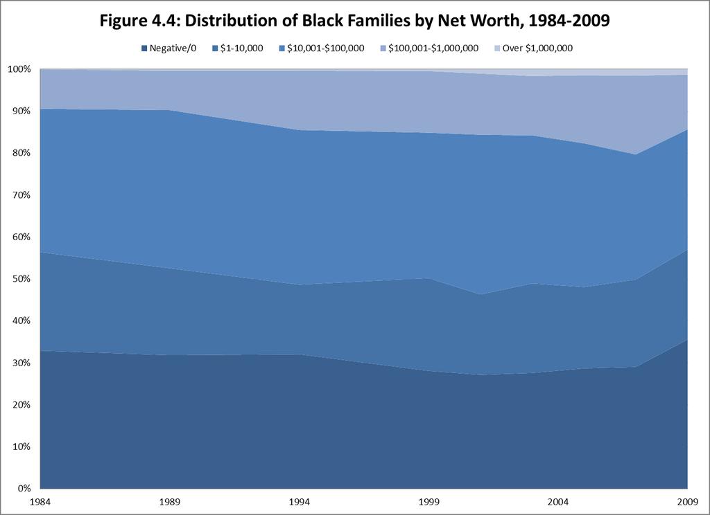
112 100