Occasional Paper Series

Transcription

1 Occasional Paper Series Jan Hannes Lang, Cosimo Izzo, Stephan Fahr, Josef Ruzicka Anticipating the bust: a new cyclical systemic risk indicator to assess the likelihood and severity of financial crises No 219 / February 2019 Disclaimer: This paper should not be reported as representing the views of the European Central Bank (ECB). The views expressed are those of the authors and do not necessarily reflect those of the ECB.

2 Contents Abstract 3 Non-technical summary 4 1 Introduction 6 2 Useful early warning indicators for financial crises in EU countries Overview of the dataset for the early warning exercise A robust set of early warning evaluation criteria The best performing univariate early warning indicators 14 3 Design features of the domestic cyclical systemic risk indicator Generic procedure for constructing a tractable composite systemic risk indicator Selection of sub-indicators for the d-sri Normalisation and aggregation of d-sri sub-indicators 23 4 Assessing the likelihood and severity of crises with the d-sri Assessing the likelihood of financial crises Assessing the severity of financial crises Examples of how the d-sri has performed historically 38 5 Accounting for cross-country spill-overs 42 6 Conclusion 44 References 45 Annex 49 A.1 A primer on evaluation criteria for early warning models 49 A.2 Equivalence of the d-sri based on raw and normalised data 51 A.3 Overview of the financial crises dataset 53 A.4 Additional tables with univariate early warning results 54 A.5 Evolution of d-sri sub-indicators before crises 60 A.6 Decompositions of the benchmark d-sri 63 ECB Occasional Paper Series No 219 / February

3 A.7 Robustness of d-sri dynamics and early warning properties 65 A.8 Details on local projections and quantile regressions 73 A.9 Robustness of d-sri impulse response functions 74 ECB Occasional Paper Series No 219 / February

4 Abstract This paper presents a tractable, transparent and broad-based domestic cyclical systemic risk indicator (d-sri) that captures risks stemming from domestic credit, real estate markets, asset prices, and external imbalances. The d-sri increases on average several years before the onset of systemic financial crises, and its early warning properties for euro area countries are superior to those of the total credit-to-gdp gap. In addition, the level of the d-sri around the start of financial crises is highly correlated with measures of subsequent crisis severity, such as GDP declines. Model estimates suggest that the d-sri has significant predictive power for large declines in real GDP growth three to four years down the line, as it precedes shifts in the entire distribution of future real GDP growth and especially of its left tail. The d-sri therefore provides useful information about both the probability and the likely cost of systemic financial crises many years in advance. Given its timely signals, the d-sri is a useful analytical tool for macroprudential policymakers. Keywords: systemic risk, financial crises, early warning models, quantile regressions, local projections, GDP at risk. JEL codes: G01, G17, C22, C54. ECB Occasional Paper Series No 219 / February

5 Non-technical summary The global financial crisis has shown that the unravelling of systemic risk can have large detrimental effects on the output and welfare of societies. Hoggarth et al. (2002) find that, on average, crisis periods result in cumulative output losses of 15-20% of annual GDP. Laeven and Valencia (2012) estimate that during past banking crises across a large sample of countries worldwide, output losses amounted on average to 23% of GDP. Lo Duca et al. (2017) estimate that output losses during systemic financial crises in EU countries amounted to 8% of GDP on average. In order to prevent systemic financial crises or mitigate their impact in the future, it is essential to have measures of systemic risk that provide sufficient lead time for policymakers to act in a countercyclical manner. The total credit-to-gdp gap of the Basel III framework (the Basel gap ) 1 is a useful starting point for measuring the cyclical dimension of systemic risk. This is because various studies have shown that it provides good aggregate early warning signals for systemic banking crises. 2 However, the Basel gap has some shortcomings when it comes to measuring cyclical systemic risk. First, it can be biased downward the longer credit booms last, because credit excesses enter the trend estimate as time progresses. 3 Second, it is sensitive to the length of the underlying time series, reducing the robustness of the signal for some euro area countries, owing to short credit series of years. Third, issues of interpretation and communication may arise, as the Basel gap can decrease in situations where the credit-to-gdp ratio increases strongly, but at a slower pace than the trend component. In view of these shortcomings, complementary measures of cyclical systemic risk need to be developed. This paper presents a new domestic cyclical systemic risk indicator (d-sri) with predictive power for the likelihood and the severity of financial crises. The d-sri is a tractable, transparent and broad-based composite indicator that captures cyclical systemic risks from developments in domestic credit, real estate markets, asset prices, and external imbalances. It is designed to signal financial crisis vulnerabilities sufficiently in advance, so that mitigating macroprudential policy action could be taken. Given the high correlation between the level of the d-sri at the start of a crisis and the magnitude of subsequent GDP declines, it can also help to inform the calibration of macroprudential policy tools. The d-sri is constructed as the optimal weighted average of six early warning indicators, after normalising the individual indicators. Indicator normalisation is The Basel gap refers to the total credit-to-gdp gap, which is calculated as the cyclical component of a recursive Hodrick-Prescott (HP) filter with a smoothing parameter of 400,000 applied to the total credit-to-gdp ratio. See for example Borio and Lowe (2002), Borio and Drehmann (2009), Aldasoro, Borio and Drehmann (2018), or Detken et al. (2014). For a detailed explanation of this shortcoming, see Lang and Welz (2017). ECB Occasional Paper Series No 219 / February

6 done by subtracting the median and dividing by the standard deviation of the pooled indicator distribution across countries. Optimal indicator weights are chosen to maximise the early warning properties of the composite d-sri for systemic financial crises that are at least partly due to domestic vulnerabilities. The optimal weighting procedure for the d-sri assigns the largest weight to the bank credit-to-gdp change (36%), followed by the current account balance (20%), the residential real estate price-to-income ratio change (17%), real equity price growth (17%), the debt service ratio change (5%), and real total credit growth (5%). The d-sri starts to increase on average around four to five years ahead of systemic financial crises, with a clear pattern of increasing imbalances. It usually reached its peak value between four to eight quarters before the onset of past systemic financial crises in euro area countries, Denmark, Sweden and the United Kingdom. Both the in-sample and the out-of-sample early warning properties of the d-sri are superior to those of the credit-to-gdp gap and other well-performing univariate early warning indicators. The early warning properties and dynamics of the d-sri are robust to real-time indicator normalisation and real-time estimation of optimal weights for combining the sub-indicators. The level of the d-sri around the start of systemic financial crises is highly correlated with measures of crisis severity, such as real GDP declines. There is a high negative correlation (-0.67) between the maximum value of the d-sri before the start of a systemic financial crisis and the maximum drop in real GDP during the ensuing crisis. There is a similar pattern, in the opposite direction, for the maximum level of the d-sri at the start of systemic financial crises and subsequent increases in the unemployment rate. For the 19 systemic financial crises in euro area countries, Denmark, Sweden and the United Kingdom for which d-sri data are available, larger non-financial private sector imbalances, as measured by the level of the d-sri, therefore tended to be associated with more severe financial crises. Econometric model estimates show that high d-sri values contain information about large declines in real GDP growth and in particular about downward shifts in the left tail of the GDP growth distribution many years in advance. An increase in the d-sri by one standard deviation implies on average a decline in future real GDP growth of around 4 percentage points three to four years into the future. The power of the d-sri to predict future real GDP drops is statistically significant between horizons of 9 to 20 quarters ahead, suggesting that high current d-sri values predict prolonged future declines in real GDP growth. The paper further shows that the drop in average real GDP growth is due to a shift in the entire real GDP growth distribution, and especially in its left tail. For a horizon of 11 to 18 quarters ahead, a one-standard-deviation value of the d-sri predicts a reduction in the 10th percentile of the conditional real GDP growth distribution by around -5 percentage points, compared to a range of -2 to -4 percentage points for the 75th and 25th percentile. To summarise, the d-sri provides useful information about the probability and likely economic costs of a financial crisis many years in advance. Given its timely signals of domestic cyclical systemic risk, it is a useful analytical tool for macroprudential policymakers. ECB Occasional Paper Series No 219 / February

7 1 Introduction The global financial crisis has shown that the unravelling of systemic risk can have large detrimental effects on output and the welfare of societies. Hoggarth et al. (2002) find that, on average, crisis periods result in cumulative output losses of 15-20% of annual GDP. Laeven and Valencia (2012) estimate that output losses during past financial crises across a large sample of countries worldwide amounted on average to 23% of GDP. Lo Duca et al. (2017) estimate that output losses during past systemic financial crises in EU countries amounted to 8% of GDP on average. Although systemic financial crises are rare events, these figures show that preventing such crises or mitigating the resulting losses should have a positive impact on the welfare of societies. Indicators of systemic risk can provide policymakers with useful information on the financial stability conditions of the economy and the financial system. Academics and policy institutions alike have often focused on tracking financial stress indicators that rely predominantly on market-based valuations (see Giglio et al. (2016), Holló et al. (2012), Benoit et al. (2016), Aikman et al. (2017)). The large body of literature on stress indicators covers a broad range of risk aspects of individual financial institutions, as well as in the aggregate, and provides indications of the extent to which specific risk factors contribute to overall stress levels. However, these methods nevertheless fall short of providing policymakers advance signals of the build-up of systemic risk, as most of them tend to be coincident, or only provide signals with short lead times ahead of crises. Leading indicators that provide signals on systemic risk sufficiently early allow policymakers to adjust the policy mix to safeguard financial stability. In the context of identifying vulnerabilities ahead of balance of payment or banking crises, early warning systems have proven simple, flexible and informative (see survey by Chamon and Crowe (2012)) 4. First, they are simple to implement because the related models only require three pieces of information: crisis dates, a set of potential signalling indicators and a methodology to combine the information contained in the indicators. Second, these models are flexible because they can be specified to signal financial crisis events with different lead times. Third, the literature has been successful in identifying useful indicators for signalling the build-up of vulnerabilities early on. The total credit-to-gdp gap ( Basel gap ) 5 is a useful first summary measure for characterising the cyclical variations of systemic risk preceding financial crises. This has been established in various studies by Borio and Lowe (2002), Borio and Drehmann (2009) and Detken et al. (2014) among others. These papers establish 4 5 For additional surveys, see Frankel and Saravelos (2012), Davis and Karim (2008), and Demirgüc-Kunt and Detriagiache (2005). The Basel gap refers to the total credit-to-gdp gap, calculated as the cyclical component of a recursive Hodrick-Prescott (HP) filter with a smoothing parameter of 400,000 applied to the total credit-to-gdp ratio. ECB Occasional Paper Series No 219 / February

8 that the Basel gap is a useful measure of cyclical systemic risk, as it provides good aggregate early warning signals for systemic banking crises across a large sample of countries and time periods. However, the Basel gap has some shortcomings when it comes to measuring cyclical systemic risk. 6 First, it can be biased downward after a prolonged credit boom, because the credit excesses partly enter into the trend estimate as time progresses. 7 Second, it is sensitive to the length of the underlying time series, reducing the robustness of the signal for some euro area countries, owing to short credit series of years. Third, issues of interpretation and communication may arise, as the Basel gap can decrease in situations where the credit-to-gdp ratio increases strongly, but at a slower pace than the trend component. In view of these shortcomings, complementary measures of cyclical systemic risk need to be developed. This paper evaluates the performance of a broad set of early warning indicators and develops a new domestic systemic risk indicator (d-sri) to characterise cyclical systemic risks in euro area countries. The main contributions of this paper are threefold. First, it systematically tests for the information contained in a broad set of variables to signal systemic financial crises in EU countries many years in advance. Second, it develops a parsimonious composite indicator of cyclical systemic risk (the d-sri), which summarises the build-up of aggregate imbalances along various risk categories, and has excellent and robust early warning properties. Third, the paper illustrates the ability of the d-sri to also provide valuable information about future real GDP developments many years in advance, using local projections and quantile regressions. The main finding of the univariate early warning analysis is that simple credit and asset price indicators can have similar or even better early warning properties for systemic financial crises than the Basel gap. In particular, for euro area countries plus Denmark, Sweden and the United Kingdom, bank credit indicators tend to have better early warning properties than total credit indicators. Low-frequency changes in credit-to-gdp ratios also have better signalling properties than gaps derived with a recursive HP filter. Similarly, low-frequency changes in the debt service ratio (DSR) or the residential real estate (RRE) price-to-income ratio show comparable early warning performance to the Basel gap. The findings of the univariate early warning analysis are used to inform the selection of indicators for the construction of the composite d-sri. The d-sri is constructed as a weighted average of six well-performing early warning indicators, after they are normalised to the same scale. Indicator normalisation is performed by subtracting the median and dividing by the standard deviation of the pooled indicator distribution across euro area countries and over time. The weights for the individual indicators are chosen to maximise the early warning 6 7 See Lang and Welz (2017) for an overview of some of the shortcomings of the Basel gap. For additional discussion of its shortcomings, see also Castro et al. (2016), Repullo and Saurina (2011), and Edge and Meisenzahl (2011). For a detailed explanation of this shortcoming, see Lang and Welz (2017). ECB Occasional Paper Series No 219 / February

9 properties of the d-sri for systemic financial crises in euro area countries plus Denmark, Sweden and the United Kingdom. Given the normalisation of the individual indicators, the d-sri and its subcomponents can be interpreted as deviations from their historical median expressed in units of the historical standard deviation. The strategy for selecting the d-sri sub-indicators strikes a balance between institutional requirements for monitoring systemic risk and the signalling performance of the indicators. In particular, the European Systemic Risk Board (ESRB) recommends 8 six indicator categories for monitoring the build-up of cyclical systemic risk in the context of the countercyclical capital buffer (CCyB). These indicator categories include measures of credit developments, potential property price overvaluation, external imbalances, bank balance sheet strength, private sector debt burden and mispricing of risk. Based on the results of the univariate early warning analysis, the best univariate early warning indicator is identified for each of the risk categories and included in the d-sri (the category bank balance sheet strength is not included due to limited data availability). The six d-sri indicators and their optimal weights (in brackets) are as follows: the two-year change in the bank credit-to-gdp ratio (36%), the two-year growth rate of real total credit (5%), the two-year change in the DSR (5%), the three-year change in the RRE price-to-income ratio (17%), the three-year growth rate of real equity prices (17%), and the current account-to-gdp ratio (20%). The procedure for constructing the d-sri lies between the two canonical approaches to early warning systems identified in the literature; more so, it combines expert judgment with the purely quantitative modelling strategies used so far. Surveys of the literature on early warning systems (see Bell and Pain (2000), Demirgüc-Kunt and Detriagiache (2005), and Davis and Karim (2008)) tend to categorise them into two main classes: the univariate signalling approach (Kaminsky and Reinhart (1999)) and the regression analysis approach (Demirgüc-Kunt and Detriagiache (1998), and Eichengreen and Rose (1998)). 9 The d-sri is constructed by first selecting indicators based on their univariate signalling performance, and then aggregating the indicators based on a linear regression approach. Additionally, expert judgment enters the d-sri in two steps. First, via dictating variable selection along pre-defined risk categories (identified by experts); second, by imposing a minimum weight of 5% assigned to each of the d-sri indicators. The multivariate nature of the d-sri ensures that it is broad-based, while the linear aggregation ensures that it is transparent and easy to communicate. 8 9 See ESRB recommendation ESRB/2014/1 on guidance for setting countercyclical buffer rates. However, with current early warning systems that use machine learning tools (see for example Alessi and Detken (2018) or Holopainen and Sarlin (2017) for a comparison of those techniques) this distinction is fading. One of the advantages of some of these models is the possibility of building non-linear classifiers that can account for interesting interactions among variables on the right-hand side. Nevertheless, the optimal parametrisation of the models is obtained by minimising some out-of-sample measures computed by reshuffling the dataset; and most of the conventional tools, such as standard cross-validation, assume IID data. This can be an acceptable assumption for cross-section data, but not in the case of systemic risk that evolves over time (see Varian (2014), Mullainathan and Spiess (2017) for an introduction to these tools and methods). ECB Occasional Paper Series No 219 / February

10 The empirical assessment for EU countries shows that the d-sri contains valuable information about the likelihood and severity of financial crises many years in advance. On average, the d-sri increases well above its normal level around five years ahead of past systemic financial crises in euro area countries, Denmark, Sweden and the United Kingdom. The in- and out-of-sample early warning properties are superior to those of all individual indicators assessed, including the Basel gap. In addition, the level of the country-specific d-sri around the start of past systemic financial crises is highly correlated with measures of subsequent crisis severity in the country in question, such as declines in real GDP. Estimates based on econometric tools, such as local projections or quantile regressions, suggest that high values of the d-sri predict large declines in real GDP growth about three to four years ahead. These declines are non-linear, with the greatest impact on the left tail of the GDP growth distribution. This is in line with studies by Jordà et al. (2013) and Adrian et al. (2016). In contrast to stress indicators, a key desirable property of the early warning indicators and the d-sri is that signals flare up well before crisis events hit the economy. Historical regularities indicate that the seeds of a crisis are sown well in advance, as imbalances build up over time and leave the financial system vulnerable to shocks. As this paper shows, the d-sri is a parsimonious composite indicator that tracks such a build-up of imbalances early on in the financial cycle, giving policymakers enough time to implement corrective policy measures. Macroprudential policy, as a countercyclical preventive policy, therefore benefits from these early signals issued by the d-sri, as they give financial actors ample lead time to adjust to new policy measures. The empirical properties of the d-sri make it a useful tool for the core purpose of macroprudential policy, which is to counter financial instability. The early warning models and the d-sri provide robust signals of the build-up of cyclical systemic risks and the likely economic losses in case of a crisis. Beyond being informative by itself, the d-sri can be integrated into broader empirical studies using Bayesian or threshold Vector Auto Regressions (VARs) to uncover its relationship with other macroeconomic variables. Given the d-sri s ability to predict crisis losses, it can also support the tractable calibration and selection of stress test scenarios in an integrated risk monitoring and assessment framework for macroprudential policy. The remainder of this paper describes the performance of the different early warning indicators, before presenting details of the design of the d-sri and its empirical properties across euro area countries. Section 2 describes the data and results of the comprehensive univariate early warning exercise that serves as the basis for the selection of indicators for the d-sri. Section 3 provides details of the design features of the d-sri. Section 4 discusses the information content of the d-sri about the likelihood and severity of financial crises in euro area countries. Section 5 shows how the d-sri can be extended to also account for cross-country risk spill-overs, while Section 6 concludes the paper. The Annex provides further technical details on the early warning exercise and the construction and properties of the d-sri. ECB Occasional Paper Series No 219 / February

11 2 Useful early warning indicators for financial crises in EU countries Early warning models have been increasingly used for financial stability analysis since the start of the global financial crisis. These types of models had already been used in academic work before the global crisis to study vulnerabilities preceding balance of payments problems or banking crises. 10 Since the global financial crisis and in the context of new macroprudential mandates, the ECB and other macroprudential authorities now regularly use early warning models as one of the tools for systemic risk identification. Based on the work by Borio and Lowe (2002), the early warning literature identified the Basel gap as one of the best univariate early warning indicators for banking crises. Real estate price gaps, debt service ratios, household debt and international debt have also been found to be useful early warning indicators. 11 However, there is increasing evidence that the Basel gap has shortcomings. 12 A major shortcoming is that the Basel gap is sensitive to the length of the underlying time series (see Chart 1 for an example), which is a potential issue for some countries in the euro area with data availability of only years. The out-of-sample early warning performance of the Basel gap is also less reliable than its in-sample performance (see Section 2.3). The development of additional systemic risk indicators is therefore warranted to complement the Basel gap for identifying the build-up of cyclical systemic risks ahead of crises. This section presents the results of a comprehensive evaluation exercise for a large set of early warning indicators, based on the new ECB/ESRB EU financial crises database. 13 This new database for financial crises in European countries was developed under the umbrella of the Financial Stability Committee of the Eurosystem and the Advisory Technical Committee of the ESRB with the goal to support the calibration of models for macroprudential analysis. This paper provides an extensive evaluation exercise of univariate early warning indicators based on the new crisis database. The identification of these useful early warning indicators provides the basis for constructing the composite d-sri (see Section 3). The main result of the early warning exercise is that simple credit and asset price indicators can have similar or even better early warning properties for systemic financial crises than the Basel gap. In particular, for euro area countries plus Denmark, Sweden and the United Kingdom, bank credit indicators tend to have better early warning properties than total credit indicators. Moreover, changes in See Eichengreen, and Rose (1998), Honohan (1997), Kaminsky and Reinhart (1999), Demirgüç-Kunt and Detragiache (2000), or Borio and Lowe (2002). See Borio and Lowe (2002), Alessi and Detken (2011), Drehmann and Juselius (2014), Detken et al. (2014), Aldasoro Borio and Drehmann (2018), or Tölö, Laakkonen and Kalatie (2018). See Lang and Welz (2017) for an overview of some of the shortcomings of the Basel gap. For additional discussion of its shortcomings, see Castro et al. (2016), Repullo and Saurina (2011) and Edge and Meisenzahl (2011). See Lo Duca et al. (2017) for details of this new database for financial crises in EU countries. ECB Occasional Paper Series No 219 / February

12 credit-to-gdp ratios (e.g. over a 2-year horizon) have better signalling properties than the traditional credit gaps derived from a recursive one-sided HP filter. Similarly, multi-year DSR or RRE price-to-income ratio changes show comparable early warning performance to the Basel gap. These results further confirm and sharpen those found in the early warning literature so far. The remainder of this section describes the early warning exercise and its results in greater detail. Chart 1 HP-filtered credit gaps can be highly sensitive to the starting date of the underlying time series HP-filtered credit-to-gdp gaps based on different starting dates (horizontal axis: date; vertical axis: HP-filtered bank credit-to-gdp gaps in percentage points) Sources: ECB calculations based on various data sources. Notes: The different credit gaps are based on the same underlying series for the bank credit-to-gdp ratio, but the starting date for estimating the recursive HP filter varies. 2.1 Overview of the dataset for the early warning exercise The new ECB/ESRB EU crises database is used as a basis for defining the relevant financial crisis episodes for the early warning exercise. 14 The new ECB/ESRB EU crises database provides precise chronological definitions of financial crisis periods in EU countries between 1970 and The dataset and the dating of the crisis events has been determined by combining financial stress indices and consulting financial stability experts from national and European authorities represented in the Financial Stability Committee of the Eurosystem and in the Advisory Technical Committee of the ESRB. One important innovation of the dataset is that it contains information about whether a financial stress event was systemic or not and whether the event was of purely domestic origin, purely foreign origin or due to a combination of domestic and foreign factors. This type of information is particularly useful in the context of early warning exercises, as it helps to narrow down the set of relevant crises to analyse. 14 See Lo Duca et al. (2017) for details of this new database for financial crises in EU countries. ECB Occasional Paper Series No 219 / February

13 Chart 2 The systemic financial crises used for the early warning exercise are clustered around the global financial crisis Vulnerability periods (1-8 quarters pre-crisis) for euro area countries plus Denmark, Sweden and the UK since 1970 (horizontal axis: date; vertical axis: number of countries in a vulnerable state) Sources: ECB calculations based the database described in Lo Duca et al. (2017). Notes: Vulnerability periods are defined as 1 to 8 quarters ahead of systemic financial crises that were not purely due to foreign factors. The baseline financial crisis definition for the exercise encompasses all systemic events from the ECB/ESRB crises database that were not purely due to foreign factors. This focuses the evaluation exercise on crisis events that were at least partly related to the build-up of domestic imbalances. This set of crises seems of particular relevance, as macroprudential policy tools mostly apply to domestic banking sector exposures (e.g. in the case of the countercyclical capital buffer) or to domestic agents (e.g. in the case of loan-to-value limits). The sample considered for the early warning exercise comprises all euro area countries plus Denmark, Sweden and the UK for the period Q Q Out of the 22 countries in the sample, 18 experienced at least one systemic financial crisis of macroprudential relevance, that was due to purely domestic factors or a combination of domestic and foreign factors (see Table A.1 in the Annex for details on the systemic financial crisis events across EU countries). Belgium, Luxembourg and Slovakia recorded only purely imported crises, whereas Malta had no systemic event at all. In total, there are 26 relevant crises and there is a significant clustering of 14 events during the recent global financial crisis (see Chart 2). 15 For the early warning exercise, we convert the crisis variable into vulnerability indicators that take a value of 1 during pre-specified windows before the start of a crisis, and zero otherwise. The vulnerability indicators are set to missing between the end of the specified pre-crisis window and the end of the actual crisis period. The benchmark vulnerability period for the early warning exercise is defined as 12-5 quarters before the start of a crisis, as the aim of the exercise is to identify indicators that issue warning signals with a sufficient lead time ahead of crises, to 15 We also test the robustness of the early warning results by using the dating of domestic systemic banking crises in Detken et al. (2014). ECB Occasional Paper Series No 219 / February

14 allow for possible macroprudential policy action. For robustness, we also test a longer pre-crisis horizon of 16-5 quarters. The evaluation exercise is performed for a large set of univariate early warning indicators that have been found useful in the literature. 16 In particular, the evaluation considers bank credit, total credit to the non-financial private sector (NFPS), households (HHs) and non-financial corporations (NFCs), asset prices such as residential real estate (RRE) or equity prices, RRE price-to-income and price-to-rent ratios, M3, debt service ratios (DSRs), real GDP growth, consumer price inflation, the real effective exchange rate (REER), current account balances and real short-term and long-term interest rates. 17 Various statistical transformations are tested for each of the early warning indicators in order to determine the ones that work best. In particular, the following transformations are used: one-quarter, one-year, two-year and three-year growth rates, one-quarter, one-year, two-year and three-year changes in ratios to GDP, one-sided recursive HP-filtered gaps with a smoothing parameter of 400,000 and 26,000, and the levels of the variables if deemed relevant (e.g. for REER or real interest rates). Only indicators that have at least 1,500 country-quarter observations are considered relevant for the analysis, to ensure sufficient sample coverage. 2.2 A robust set of early warning evaluation criteria The univariate early warning indicators are evaluated based on a combination of their in-sample and out-of-sample signalling performance. The in-sample early warning properties are evaluated based on the AUROC (see the Annex for details on the different evaluation metrics for early warning models that are used). 18 The AUROC is computed for pre-crisis horizons of 12-5 quarters and 16-5 quarters, based on the benchmark crisis definition from the new ECB/ESRB crises database (named 12-5 bench and 16-5 bench ) and for a pre-crisis horizon of 12-5 quarters, based on the crisis definition in Detken et al. (2014) ( 12-5 check ). The out-of-sample early warning properties are evaluated using the relative usefulness measure proposed by Sarlin (2013), based on a recursive quasi real-time exercise starting in Q for the benchmark crisis definition and pre-crisis horizon of 12-5 quarters. Optimal signalling thresholds and the relative usefulness measure are computed based on the loss See Borio and Lowe (2002), Borio and Drehmann (2009), Drehmann et al. (2011), Drehmann and Juselius (2014) and Detken et al. (2014). In order to generate long time series for Germany, data before Q refers to West Germany, while from Q onwards it refers to unified Germany. The series were linked to avoid breaks in AUROC stands for Area Under the Receiver Operating Characteristics Curve. It is a global measure of the early warning performance of an indicator. A perfect indicator has an AUROC of 1 and an uninformative indicator an AUROC of 0.5. ECB Occasional Paper Series No 219 / February

15 function proposed by Alessi and Detken (2011) and balanced policy preferences between missing crises and issuing false alarms. 19 The final ranking of univariate early warning indicators assigns a weight of two-thirds to a weighted average in-sample AUROC and a weight of one-third to the out-of-sample relative usefulness measure. Initially, a weighted average in-sample AUROC is computed that assigns weights of 50%, 35% and 15% respectively to the AUROCs for the three different vulnerability indicators 12-5 bench, 16-5 bench and 12-5 check. This weighting is chosen to give prominence to the 12-5 bench vulnerability indicator while also ensuring robustness. Two rankings are then assigned to each indicator for the weighted average AUROC and the out-of-sample relative usefulness respectively. A final ranking is computed based on a weighted average of the two rankings for the in-sample and out-of-sample performance, using weights of two-thirds and one-third respectively. In this way the final ranking of each indicator takes into account different prediction horizons, in- and out-of-sample performance and different crisis definitions. 2.3 The best performing univariate early warning indicators The main result of the evaluation exercise is that simple transformations of credit and asset price variables can have similar or even better early warning properties than the Basel gap. 20 In particular, for the euro area countries plus Denmark, Sweden and the UK, changes in, or real growth rates of, bank credit, household credit, total credit, NFC credit, M3, the DSR or the house-price-to-income ratio, all have a higher in-sample AUROC and out-of-sample usefulness than the Basel gap (Table 1). The best univariate signalling indicators tend to have in-sample AUROCs of more than 0.80 and an out-of-sample relative usefulness of around 40% (Table A.2 in the Annex compares the top 25 univariate signalling indicators). By comparison, the Basel gap has a weighted average in-sample AUROC of 0.71 and a much lower out-of-sample relative usefulness of 13%. Simple bank credit and household credit transformations tend to have the best early warning properties and outperform indicators that are based on total credit or NFC credit (Table 1). In particular, among the top 25 univariate early warning indicators, the first seven are related to medium-term changes in the bank credit-to-gdp ratio and the HH credit-to-gdp ratio (Table A.2 in the Annex). The two-year change in the bank credit-to-gdp ratio is the best indicator, with a weighted average AUROC of 0.83 and an out-of-sample relative usefulness of 38%. It is The recursive exercise is performed as follows: Starting in 2000q1, a univariate signalling model is estimated using data up to 1997q1. The resulting optimal signalling threshold, based on balanced preferences between missing crises and issuing false alarms is applied to data from 2000q1 to generate a signal. Once the signal is recorded, the same procedure is performed for the next quarter, i.e. 2000q2, where the relevant estimation sample for the univariate signalling model now includes one additional quarter of data, i.e. data up to 1997q2. This procedure is performed recursively until 2016q4. The Basel gap has been found to be one of the best univariate early warning indicators for financial crises in previous studies (see Borio and Drehmann (2009), Drehmann and Juselius (2014) and Detken et al. (2014)), taking on a central role in relation to guiding decisions about the countercyclical capital buffer within the Basel III framework (see Basel Committee for Banking Supervision (2010) and ESRB recommendation 2014/1). ECB Occasional Paper Series No 219 / February

16 followed by the two-year change in the HH credit-to-gdp ratio, with an in-sample AUROC of 0.80 and an out-of-sample relative usefulness of 42%. By comparison, the best transformations of total credit (one-year change in the ratio to GDP) and NFC credit (one-year real growth) have an in-sample AUROC of around 0.75 and an out-of-sample relative usefulness of 25% (Table 1). Table 1 Simple credit and asset price indicators can have similar or even better early warning properties for systemic financial crises than the Basel gap Best indicator for each variable category based on a weighted average of in-sample and out-of-sample performance Indicator Final Ranking [Weighted average ranking (1/3 to out-of-sample and 2/3 to in-sample)] Rank based on weighted average (50%-35%-15%) Weighted average (rel. weights 50%-35%-15%) In- sample 12-5 check AUROC (rel. weight of 15%) 12-5 bench AUROC (rel. weight of 50%) 16-5 bench AUROC (rel. weight of 35%) Out-of-sample Rank by relative usefulness Relative Usefulness I Bank credit to NFPS as % of GDP, 2-year change 1 [3] II Total credit to HHs as % of GDP, 2-year change 3 [5.7] III Debt service ratio, 2-year change 8 [11.7] IV Monetary aggregate M3, 3-year real growth 12 [15.3] V Total consolidated credit as % of GDP, 1-year change 15 [24.7] VI Total consolidated credit to NFCs, 1-year real growth 18 [29.3] VII House price-to-income ratio, 3-year change 27 [36.3] VIII Current account balance as % of GDP 41 [45.7] IX Equity price, 3-year real growth 56 [58] X Basel gap: Total credit as % of GDP, GAP (400'000) 59 [58.3] Source: ECB calculations based on the ECB/ESRB financial crises database described in Lo Duca et al. (2017). Notes: AUROC stands for Area Under the Receiver Operating Characteristics Curve. It is a global measure of the early warning performance of an indicator. A perfect indicator has an AUROC of 1 and an uninformative indicator an AUROC of 0.5. The in-sample AUROC is computed for pre-crisis horizons of 12-5 quarters and 16-5 quarters, based on the benchmark crisis definition from the new ECB/ESRB EU database (named 12-5 bench and 16-5 bench ), and for a pre-crisis horizon of 12-5 quarters, based on the crisis definition in Detken et al (named 12-5 check ). The out-of-sample early warning properties are evaluated using the relative usefulness measure for balanced preferences, based on a recursive quasi real-time exercise for the pre-crisis horizon 12-5 bench starting in Q The final ranking of univariate early warning indicators assigns a weight of two thirds to the ranking based on a weighted average in-sample AUROC, and a weight of one third to the ranking based on the out-of-sample relative usefulness. The weighted average AUROC (AUROC ) assigns weights of 50%, 35% and 15% respectively to the AUROCs for the vulnerability indicators 12-5 bench, 16-5 bench and 12-5 check. The annex has details of the evaluation criteria for early warning models. The Basel gap refers to the standardised credit-to-gdp gap, which is obtained as the cyclical component of a recursive HP filter with a smoothing parameter of 400,000 applied to the total credit-to-gdp ratio. For credit variables, changes in credit-to-gdp ratios tend to have superior early warning properties than real growth rates or gap measures based on a recursive HP filter (see Chart 3). For bank credit, total credit and household credit, the in-sample AUROCs of changes in credit-to-gdp ratios ( ) tend to be considerably higher than those based on real growth rates ( ), while the in-sample performance of growth rates and gaps tends to be similar (Tables A 3 to A 5 in the Annex). Moreover, the out-of-sample performance of changes in credit-to-gdp ratios and real growth rates tends to be similar (25%-42%), while the out-of-sample ECB Occasional Paper Series No 219 / February

17 performance of gaps tends to be much weaker (12%-22%). 21 Transformations based on changes in credit-to-gdp ratios therefore tend to be ranked highest within each of the credit categories. The exception to this is NFC credit, where the one-year real growth rate performs slightly better than the one-year change in the credit-to-gdp ratio. Chart 3 For euro area countries changes in the bank credit- and the household credit-to-gdp ratios are the best univariate early warning indicators; they perform better than total credit indicators or HP-filtered gap measures In-sample AUROC and out-of-sample relative usefulness for different credit-related early warning indicators (x-axis: variable name [variable ranking]; y-axis: AUROC and relative usefulness) AUROC 12-5 check AUROC 12-5 bench AUROC 16-5 bench Relative Usefulness Out-of-sample Bank credit to NFPS as % of GDP, 2- year change [3] Household credit as % of Real bank credit to Total consolidated GDP, 2-year NFPS, 2-yearcredit as % of change [5.7] growth [14.7] GDP, 1-year change [24.7] Real consolidated credit to NFCs, 1-year growth [29.3] Bank creditto-gdp gap [36.7] Real total credit, 2-year growth [40] Household credit-to-gdp gap [42.7] Total creditto-gdp gap (Basel gap) [58.3] 0.10 Sources: ECB calculations based on the ECB/ESRB EU financial crises database described in Lo Duca et al. (2017). Notes: AUROC stands for Area Under the Receiver Operating Characteristics Curve. It is a global measure of the early warning performance of an indicator. A perfect indicator has an AUROC of 1 and an uninformative indicator an AUROC of 0.5. The in-sample AUROC is computed for pre-crisis horizons of 12-5 quarters and 16-5 quarters based, on the benchmark crisis definition from the new ECB/ESRB EU database (named 12-5 bench and 16-5 bench ), and for a pre-crisis horizon of 12-5 quarters based on the crisis definition in Detken et al (named 12-5 check ). The out-of-sample early warning properties are evaluated using the relative usefulness measure for balanced preferences, based on a recursive quasi real-time exercise for the pre-crisis horizon 12-5 bench starting in Q The final ranking of univariate early warning indicators assigns a weight of two thirds to the ranking based on a weighted average in-sample AUROC and a weight of one third to the ranking based on the out-of-sample relative usefulness. The weighted average AUROC assigns weights of 50%, 35% and 15% respectively to the AUROCs for the vulnerability indicators 12-5 bench, 16-5 bench and 12-5 check. The Annex has details of the evaluation criteria for early warning models. Changes in the bank credit-to-gdp ratio tend to accelerate around five years before the start of systemic financial crises, usually peaking around one to two years before a crisis materialises (see Chart 4). The two-year change in the bank credit-to-gdp ratio usually increased markedly above its median during the five years preceding past financial crisis episodes (see cross-country mean or interquartile range around financial crises). By comparison, the Basel gap showed a persistently elevated pattern during the six years before past systemic financial crises, with no marked 21 One exception is that the out-of-sample performance of HH credit-to-gdp changes is quite a bit better than that of real HH credit growth. ECB Occasional Paper Series No 219 / February

18 variation to indicate the timing of a crisis (see Chart 5). Indeed, the 25th percentile of the Basel gap during pre-crisis periods was virtually identical to the historical median during normal times, thus offering a less robust signal ahead of crises. Charts 4 and 5 show that the two-year change in the bank credit-to-gdp ratio is better able to distinguish pre-crisis times from normal times than the Basel gap. Chart 4 The 2-year change in the bank credit-to-gdp ratio starts to increase around five years before a crisis, with a clear pattern showing increasing imbalances Cross-country distribution of the 2-year change in the bank credit-to-gdp ratio around systemic financial crises (x-axis: quarters before/after start of a crisis; y-axis: pp change) Sources: ECB calculations based on the ECB/ESRB financial crises database. Notes: The blue shaded area indicates the interquartile range of the indicator across euro area countries plus Denmark, Sweden and the UK during the quarters before and after systemic financial crises. The green line indicates the median of the indicator across the same set of countries in normal times (not within +/- six years of the start of a systemic financial crisis). The dating of systemic financial crises in the chart is based on the ECB/ESRB crises database described in Lo Duca et al. (2017). Purely foreign-induced crises are excluded. Changes in the DSR and real M3 growth also have good early warning properties and perform slightly better than total credit or NFC credit indicators (Table 1). The two-year change in the DSR has a weighted average AUROC of 0.77 and an out-of-sample usefulness of 34%. Three-year real M3 growth has similar values of 0.74 and 41%. Real M3 growth rates are among the best performing indicators out-of-sample (Table A.2 in the Annex). By comparison, the Basel gap has a weighted average in-sample AUROC of 0.71 and an out-of-sample relative usefulness of 13%. Medium-term changes in the price-to-income ratio are the best residential real estate indicators, performing slightly better than the Basel gap (Table 1). The three-year change in the RRE price-to-income ratio has a weighted average AUROC of 0.73 and an out-of-sample relative usefulness of 21%. By comparison, the three-year real growth rate of RRE prices has values of 0.70 and 22% (Table A.9 in the Annex). Due to limited data availability before 1995, it is not possible to perform the out-of-sample exercise for the RRE valuation measures. However, these valuation measures show very good in-sample performance, especially the asset-pricing approach, with AUROCs of close to or above 0.80, comparable to the in-sample performance of the best indicators. ECB Occasional Paper Series No 219 / February

19 Chart 5 The Basel gap is persistently elevated during pre-crisis periods, without a clear pattern showing increasing imbalances Cross-country distribution of the total credit-to-gdp gap (Basel gap) around systemic financial crises (x-axis: quarters before/after start of a crisis; y-axis: deviation from one-sided HP trend) Sources: ECB calculations based on the ECB/ESRB financial crises database. Notes: The blue shaded area indicates the interquartile range of the indicator across euro area countries plus Denmark, Sweden and the UK during the quarters before and after systemic financial crises. The green line indicates the median of the indicator across the same set of countries in normal times (not within +/- six years of the start of a systemic financial crisis). The dating of systemic financial crises in the chart is based on the ECB/ESRB crises database described in Lo Duca et al. (2017). Purely foreign-induced crises are excluded. The in-sample performance of the current account balance relative to GDP is similar to that of the Basel gap, but its out-of-sample performance is better (Table 1). In particular, the current account balance has a weighted average in-sample AUROC of 0.70 and a relative usefulness out-of-sample of The ratio itself has better early warning properties than changes in the ratio (see Table A.10 in the Annex). The in-sample performance of real three-year equity price growth is much lower than that of the Basel gap, but it ranks among the best indicators out-of-sample (Table 1). Its weighted average AUROC is only 0.65, while the out-of-sample relative usefulness of 42%, is the second best of all indicators. Both the in-sample and out-of-sample performance of gap measures based on equity prices is weaker than the performance of the three-year real equity price growth rate (see Table A.9 in the Annex). The Annex contains detailed tables showing the performance of all indicators, and charts that illustrate the evolution of the most important indicators before crises. In particular, Tables A.3 to A.10 show the rankings of different early warning indicators grouped by indicator category. The results of the comprehensive early warning exercise are used in the next section to inform the selection of indicators for the construction of the d-sri. Charts A.1 to A.6 in the Annex already illustrate the common patterns of these early warning indicators ahead of past systemic financial crises. ECB Occasional Paper Series No 219 / February

20 3 Design features of the domestic cyclical systemic risk indicator Individual early warning indicators capture specific aspects of the financial cycle. This section describes the construction of a composite measure of the financial cycle, namely the domestic cyclical systemic risk indicator (d-sri). The first part of this section outlines the generic procedure for aggregating variables into a composite systemic risk indicator, which can be applied to different sectors of the economy or different systemic risk categories. This generic procedure is then applied to construct the d-sri, which measures cyclical systemic risks that originate from the domestic non-financial private sector of a country. The second part of this section explains the specific selection criteria for the six sub-indicators of the d-sri. The third part provides details on the normalisation and aggregation procedure for the d-sri. 3.1 Generic procedure for constructing a tractable composite systemic risk indicator This sub-section presents a generic procedure for constructing a broad-based systemic risk indicator that is tractable, transparent, and easily interpretable for policy use. Tractability and transparency are considered to be important characteristics for a composite systemic risk indicator in order to make it easier to interpret and communicate systemic risk signals. Furthermore, policy action using granular macroprudential instruments requires means to easily identify the drivers behind risk signals in order to address the specific sources of systemic risk. The generic procedure has four building blocks and combines methods employed in the early warning literature with a simple and intuitive aggregation method. The four general building blocks are: (i) selection of a set of relevant indicator categories for the risk of interest; (ii) selection of the optimal early warning indicator for each of the indicator categories; (iii) normalisation of each optimal early warning indicator based on the pooled median and standard deviation across countries and time; and (iv) linear aggregation of the normalised early warning indicators into a composite systemic risk indicator based on optimal indicator weights. The generic composite systemic risk indicator (SRI) is defined as a weighted average of the normalised sub-indicators: K SRI i,t = ω j j=1 j x i,t j where x i,t j = x i,t x M j j x SD represents the normalised sub-indicator, with i indicating a country, t the time period, and j the sub-indicator. ω j represents the relative weight in the composite indicator attributed to the specific sub-indicator. ECB Occasional Paper Series No 219 / February

21 Normalisation is achieved by subtracting the median and dividing by the standard deviation of the pooled dataset. The median rather than the mean is chosen for normalisation, as it is more robust to outliers and ensures that a zero value of the normalised indicator can be interpreted as a normal level, with 50% of past observations being above that value and 50% below it. The standard deviation rather than the interquartile range is used for normalisation as it facilitates communication due to wider public awareness of the concept of standard deviation. As shown in the Annex, indicator normalisation does not change the dynamics or the early warning properties of the composite indicator compared to using the raw underlying data. The specific choice of moments for normalisation is therefore mainly done to facilitate communication of results. The weights for aggregating sub-indicators are chosen to optimise the early warning properties of the composite systemic risk indicator. The optimal sub-indicator weights ω j are obtained by running a linear regression of a crisis vulnerability indicator on the normalised sub-indicators and by using the estimated coefficients as weights after constraining them to sum to This regression approach provides the optimal linear combination of the underlying sub-indicators to identify vulnerable periods. Optimal country-specific weights are difficult to estimate due to the scarcity of crises at the country level. Pooled indicator normalisation and constant weights across countries and time implicitly assumes that there are common indicator patterns across the crises experienced by individual countries at different points in time which can help identify the build-up of systemic risk. This pooled approach hedges against overfitting for specific individual crises. The generic procedure for constructing a composite systemic risk indicator can be applied to different sectors of the economy or different systemic risk categories. By varying the crisis episodes of interest and the relevant categories for the early warning indicators, the focus of the systemic risk indicator can be adjusted. For example, in the context of domestic cyclical systemic risks, relevant indicator categories would include credit developments, real estate markets or asset prices, while the relevant set of crises should only include events that were induced at least partly by domestic vulnerabilities. For monitoring systemic risks within the banking sector, indicator categories could include capital adequacy, liquidity or asset quality, and the relevant set of crises should only include events that were related to banking sector problems. The following two sub-sections describe how the generic procedure outlined above is used to construct the d-sri. The d-sri is a broad-based yet tractable composite indicator that measures cyclical systemic risks that originate from the domestic non-financial private sector of a country. 22 The optimal sub-indicator weights are computed by dividing each regression coefficient by the sum of all estimated regression coefficients. This procedure ensures that weights sum to 1. For the application of this generic procedure to the measurement of domestic cyclical systemic risks (i.e. the domestic systemic risk indicator presented in this paper), a minimum weight of 5% for each sub-indicator is imposed. ECB Occasional Paper Series No 219 / February

22 3.2 Selection of sub-indicators for the d-sri Five indicator categories are included in the d-sri that cover the key categories recommended by the ESRB for monitoring cyclical systemic risks. 23 Basel Committee on Banking Supervision (BCBS) guidance, the Capital Requirements Directive (CRD IV) and ESRB Recommendation ESRB/2014/1 assign a central role to the credit-to-gdp gap for measuring cyclical systemic risks. However, additional indicator categories can cover other dimensions of cyclical systemic risks and complement signals from the Basel gap. The d-sri is therefore designed to cover five of the indicator categories for cyclical systemic risks that are recommended by the ESRB (see ESRB/2014/1): 24 (i) (ii) measures of potential overvaluation of property prices; measures of credit developments; (iii) measures of external imbalances; (iv) measures of private sector debt burden; (v) measures of potential mispricing of risk. As a rule, the d-sri includes one indicator per recommended category. The exception to this rule is credit: two indicators, one based on bank credit and the other based on total credit, are included in the d-sri. This choice is guided by the fact that credit has historically played a prominent role in driving financial crisis vulnerabilities, as documented by Schularick and Taylor (2012). The reason for including a bank credit and a total credit variable in the d-sri is to enhance its robustness to potential changes in the financial structure of a country over time. The d-sri therefore contains six indicators in total. For each indicator category, the best univariate early warning indicator is selected as the relevant d-sri sub-indicator. The results of the comprehensive early warning exercise described in Section 2 are used as the basis for selecting d-sri sub-indicators. To recall, each early warning indicator is evaluated based on a combination of the in-sample and out-of-sample signalling performance and different financial crisis definitions and prediction horizons. The final ranking of univariate early warning indicators assigns a weight of two thirds to the in-sample performance and a weight of one third to the out-of-sample performance. Tables A.3 to A.10 in the Annex provide an overview of the best early warning indicators for each of the indicator categories considered. For the two credit indicators of the d-sri, the best bank credit For details on the indicator categories recommended for risk monitoring, see recommendation C of the ESRB recommendation on guidance for setting countercyclical buffer rates (ESRB/2014/1). Indicator category (d) measures of the strength of bank balance sheets was not included in the d-sri because it is not a measure of risk build-up or imbalances per se, but more a measure of resilience of the banking sector. Category (g) measures derived from models that combine the credit-to-gdp gap and a selection of the above measures is covered by the d-sri itself. ECB Occasional Paper Series No 219 / February

23 and total credit indicators are chosen, subject to the constraint that one of them is a growth rate. 25 To summarise, the d-sri includes six useful early warning indicators related to credit, real estate, financial markets and external imbalances (see Chart 6). The specific optimal univariate early warning indicators that were selected for the d-sri based on the comprehensive early warning exercise are: (i) (ii) the two-year change in the bank credit-to-gdp ratio; the two-year growth rate of real total credit; (iii) the two-year change in the debt-service-ratio; (iv) the three-year change in the RRE price-to-income ratio; (v) the three-year growth rate of real equity prices; (vi) the current account-to-gdp ratio. All of the d-sri sub-indicators are measured in either two-year or three-year transformations as these are found to have the best early warning properties. In particular, these medium-term transformations tend to perform better than shorter-term transformations or than HP-filtered gaps (see Tables A.3-A.10 in the Annex). 26 Apart from better early warning performance, a major advantage of medium-term changes and growth rates compared to HP-filtered gaps is that they are robust to the length of the underlying time series and can be reliably computed in real-time as long as two to three years of data are available. The d-sri sub-indicators are all expressed as annualised averages, e.g. three-year changes are divided by 3 and two-year changes are divided by 2. Most of the d-sri sub-indicators have similar or even better early warning properties for systemic financial crises than the Basel gap (see Chart 6). For example, the two-year change in the bank credit-to-gdp ratio, the two-year change in the DSR and the three-year change in the RRE price-to-income ratio all attain higher in-sample AUROCs and out-of-sample relative usefulness than the Basel gap. The two-year growth rate of real total credit displays similar early warning performance to the Basel gap. The current account balance and the three-year real equity price growth rate have lower in-sample AUROCs than the Basel gap, although the equity variable attains a much higher out-of-sample relative usefulness. The risk indicators selected for the d-sri are also in line with the types of indicators that are suggested by Tölö et al. (2018) as being useful for the different risk categories suggested by ESRB recommendation ESRB/2014/1 or with the ones employed by Aikman et al. (2018) This should ensure that the information contained in the two credit indicators of the d-sri is complementary. The use of such simple medium-term transformations for filtering is also supported by the findings in Hamilton (2017), who argues forcefully against using the HP filter. ECB Occasional Paper Series No 219 / February

24 Chart 6 Most of the six d-sri sub-indicators have similar or even better early warning properties than the Basel gap for the set of euro area countries plus Denmark, Sweden and the United Kingdom In-sample AUROC and out-of-sample relative usefulness for the d-sri sub-indicators and the Basel gap (x-axis: variable name [variable ranking]; y-axis: AUROC and relative usefulness) AUROC 12-5 check AUROC 12-5 bench AUROC 16-5 bench Relative Usefulness Out-of-sample Bank credit to NFPS as % of GDP, 2-year change [3] Debt service ratio, 2-year change [11.6] RRE price-toincome ratio, 3- year change [36.3] Total real credit, 2-year growth [40] Current Account to GDP ratio [45.6] Real equity prices, 3-year growth [58] Total credit-to- GDP gap (Basel gap) [58.3] 0.10 Sources: ECB calculations based on the ECB/ESRB EU crises database described in Lo Duca et al. (2017). Notes: AUROC stands for Area Under the Receiver Operating Characteristics Curve. It is a global measure of the early warning performance of an indicator. A perfect indicator has an AUROC of 1 and an uninformative indicator an AUROC of 0.5. The in-sample AUROC is computed for pre-crisis horizons of 12-5 quarters and 16-5 quarters based on the benchmark crisis definition from the new ECB/ESRB EU database (named 12-5 bench and 16-5 bench ) and for a pre-crisis horizon of 12-5 quarters based on the crisis definition in Detken et al (named 12-5 check ). The out-of-sample early warning properties are evaluated with the relative usefulness for balanced preferences based on a recursive quasi real-time exercise for the pre-crisis horizon 12-5 bench that starts in Q The final ranking of univariate early warning indicators assigns a weight of two thirds to the ranking based on a weighted average in-sample AUROC and a weight of one third to the ranking based on the out-of-sample relative usefulness. The weighted average AUROC assigns weights of 50%, 35% and 15% respectively to the AUROCs for the vulnerability indicators 12-5 bench, 16-5 bench, and 12-5 check. The Annex contains details on the evaluation criteria for early warning models. The six well-performing d-sri sub-indicators provide a tractable, transparent and quantitative starting point for a consistent cyclical systemic risk assessment across euro area countries. The next sub-section outlines how the six d-sri sub-indicators are normalised and aggregated in an optimal way into the composite d-sri. 3.3 Normalisation and aggregation of d-sri sub-indicators The d-sri is constructed as the optimal weighted average of the six early warning indicators after they are normalised to the same scale. Indicator normalisation is performed based on moments from the pooled indicator distribution. Optimal indicator weights are chosen to maximise the early warning properties of the composite d-sri for systemic financial crises that are at least partly due to domestic vulnerabilities. ECB Occasional Paper Series No 219 / February

25 The d-sri sub-indicators are normalised by subtracting the median and dividing by the standard deviation of the pooled indicator distribution across euro area countries. Table 2 shows the relevant pooled data moments used for normalisation. It is important to reiterate that this normalisation based on pooled data moments does not alter the dynamics or the early warning properties of the d-sri compared to using the raw underlying early warning indicators to compute the d-sri (see the Annex for a formal proof of this equivalence). However, the advantage of this normalisation is that the units of the d-sri have an intuitive interpretation as the weighted average deviation from the historical median, measured in multiples of the historical standard deviation. Due to normalisation, the d-sri weights also have a direct interpretation as the contribution of each sub-indicator to the variation of the d-sri. Table 2 The 2-year change in the bank credit-to-gdp ratio has the largest d-sri weight of more than one third Overview of data moments and early warning properties of the d-sri and its sub-indicators (d-sri weights in %; data moments in either percent or percentage points) ESRB risk category Indicator Benchmark d-sri weight d-sri weight ex. equity d-sri weight ex. current account Median Standard deviation 75th percentile 90th percentile In-sample AUROC 12-5q Observations (a) measures of overvaluation of property prices (b) measures of credit developments 3-year change in RRE price-to-income ratio, p.p. 2-year change in the bank credit-to-gdp ratio, p.p. 17% 23% 21% ,867 36% 45% 52% ,282 (b) measures of credit developments 2-year growth rate of real total credit (CPI deflated), % 5% 5% 5% ,430 (c) measures of external imbalances (e) measures of private sector debt burden (f) measures of potential mispricing of risk (g) measures derived from models Current account-to-gdp ratio, % 2-year change in the debt-service-ratio (DSR), p.p. 3-year growth rate of real equity prices (CPI deflated), % Domestic Systemic Risk Indicator (d-sri) 20% 22% ,354 5% 5% 5% ,125 17% - 17% , ,658 Basel gap Total credit-to-gdp gap, p.p ,531 Alternative gap Bank credit-to-gdp gap, p.p ,452 Sources: ECB calculations based on various data sources. The weights for aggregating the d-sri sub-indicators are common across countries and time and are chosen to optimise the early warning properties of the d-sri. The procedure for estimating optimal weights follows the generic method described in Section 3.1. Given that the d-sri should provide early signals of the build-up of domestic imbalances, the vulnerability indicator for the regression to obtain optimal weights is defined as 12-5 quarters before the start of systemic financial crises from the ECB/ESRB EU crises database that are not purely due to foreign factors. Optimising the d-sri weights for such a medium-term prediction horizon ensures that signals are issued with a sufficient lead time to allow for potential policy action. The regression is estimated for all euro area countries plus Denmark, Sweden, and the United Kingdom from Q to Q (see Chart 7 for data coverage). ECB Occasional Paper Series No 219 / February

26 Chart 7 Data availability for the d-sri varies considerably across countries: it starts as early as the mid-1970s and as late as the mid-2000s for some countries Data availability of the d-sri and overview of the benchmark vulnerability indicator (x-axis: date; y-axis: country) Sources: ECB calculations based on various data sources. Notes: In blue: data coverage of the d-sri. In yellow: tranquil periods (all the observations left after excluding the crisis periods and up to 12 quarters before its start). In red: vulnerability periods (12-5 quarters before the start of systemic financial crises that are not purely due to foreign factors taken from the ECB/ESRB EU crises database). For each country, the start date of the series together with the total number of effective observations are reported, which are computed by counting observations present for both the d-sri and the 12 to 5 vulnerability indicator. The optimal weighting scheme for the d-sri based on the full sample of data assigns the largest weight to the bank credit-to-gdp change (Table 2). In particular, the optimal weight of the change in the bank credit-to-gdp ratio is 36% for the benchmark d-sri. The sub-indicators with the next highest weights are the current account to GDP ratio (20%), the RRE price-to-income change (17%), and the real equity price growth rate (17%). The DSR change and the real total credit growth rate both have weights of 5%, which is the minimum imposed for each d-sri sub-indicator. Table 2 also shows how the optimal weights change when either the equity price sub-indicator or the current account sub-indicator is excluded from the d-sri. In both cases, mainly the optimal weight assigned to the bank credit-to-gdp change increases, whereas the weights for the other sub-indicators remain at similar levels. Pooled normalisation and constant weights across countries and time ensure that the d-sri is tractable, transparent and consistent across countries. Using the pooled distribution for standardisation instead of the country-specific distribution can also make the d-sri more robust by exploiting cross-country heterogeneity. 27 For 27 Based on the assumption that countries share similar structural features, cross-country heterogeneity substitutes for longer time series. ECB Occasional Paper Series No 219 / February

27 example, a transition economy might experience long periods of high credit growth. However, these high credit growth rates may no longer be the relevant guide for the future once economic convergence has sufficiently advanced. Hence, while using pooled data can potentially disregard structural differences across countries, it can help to alleviate the sample selection bias due to short data histories for a given country. Indeed, robustness tests in the Annex show that the real-time early warning properties of the d-sri are better if the pooled distribution is used for normalisation instead of the country-specific distribution. In summary, the d-sri aggregates six early warning indicators into a broad-based indicator that captures the build-up of cyclical systemic risks early on. Compared to more complex logit early warning models or composite indicators that use time-varying weights (e.g. based on time-varying cross-correlations), the d-sri is more transparent and easier to interpret. Moreover, given that the d-sri is a linear combination of the underlying sub-indicators, its decomposition into the underlying driving factors is straightforward. This is a useful feature of the d-sri that can help identify driving factors of the cyclical systemic risk build-up and help create an overall risk narrative. Composite indicators that are similar to the d-sri are used by some EU countries to complement signals from the Basel gap in order to identify cyclical systemic risks. For example, the National Bank of Slovakia (NBS) and the Czech National Bank (CNB) have set positive countercyclical capital buffer (CCyB) rates in the past based on synthetic composite risk indicators. The CNB s financial cycle indicator 28 includes nine variables that cover credit growth, property prices, credit conditions for households and NFCs, debt sustainability of NFCs and households, asset prices and the current account as a basis for a non-linear buffer guide. The NBS s cyclogram 29 aggregates six core variables and seven supplementary variables that cover among others credit growth, housing affordability, debt burdens, lending conditions, and loan-to-value ratios. The aggregation of different risk indicators into a composite cyclical systemic risk indicator is therefore already applied by some EU countries in the CCyB policy context See Plašil et al. (2015). See Rychtarik (2014). ECB Occasional Paper Series No 219 / February

28 4 Assessing the likelihood and severity of crises with the d-sri This section shows that the d-sri contains useful information about both the likelihood and the severity of financial crises with a lead time of several years. The first sub-section documents that the d-sri has very good in-sample and out-of-sample early warning properties across euro area countries plus Denmark, Sweden and the United Kingdom. In particular, the d-sri displays long cycles and starts to increase above normal levels around four to five years ahead of systemic financial crises. The second sub-section illustrates that the d-sri also has high predictive power for large declines in future real GDP growth. In particular, quantile regression results show that the d-sri predicts a downward shift of the entire real GDP growth distribution three to four years down the road, with the most pronounced impact on the left tail of the GDP growth distribution. Finally, the third sub-section provides some country examples of how the d-sri has performed in the past. 4.1 Assessing the likelihood of financial crises The d-sri is a tractable cyclical systemic risk indicator that displays long cycles across euro area countries, Denmark, Sweden, and the United Kingdom. Chart 8 shows that the d-sri displays rather long swings that last around 10 to 15 years across countries. Since the early 1980s, the cross-country distribution of the d-sri exhibits three peaks: one at the end of the 1980s, one at the end of the 1990s, and one before the onset of the global financial crisis in 2007/2008. The first and the last peaks fall into pre-recession periods as identified by the CEPR Euro Area Business Cycle Dating Committee. The build-up of imbalances during the run-up to the global financial crisis and the subsequent bust are clearly reflected in the evolution of the d-sri across the sample of EU countries. The amplitude of both the upswing and the downswing of the d-sri around the global financial crisis were unprecedented. At the end of 2017, the d-sri still remains at subdued levels, although dispersion of the d-sri across countries remains high, with some countries already exhibiting positive values. ECB Occasional Paper Series No 219 / February

29 Chart 8 The d-sri displays long cycles with three peaks since the early 1980s across euro area countries, Denmark, Sweden, and the United Kingdom Cross-country distribution of country d-sris over time (x-axis: time; y-axis: deviation from median) Sources: ECB calculations based on various data sources and CEPR. Notes: The blue shaded area indicates the interquartile range of the d-sri across euro area countries, Denmark, Sweden, and the United Kingdom. The d-sri is constructed as a weighted average of the normalised sub-indicators, where the weights are chosen to maximise the early warning properties for systemic financial crises. Each sub-indicator is normalised by subtracting the median and dividing by the standard deviation of the indicator distribution across countries and time. The underlying indicators are: the 2-year change in the bank credit-to-gdp ratio, the 2-year growth rate of real total credit, the 2-year change in the DSR, the 3-year change in the RRE price-to-income ratio, the 3-year growth rate of real equity prices, and the current account-to-gdp ratio. Black shaded areas represent recession periods identified by the CEPR Euro Area Business Cycle Dating Committee, while grey areas represent the respective 12 to 5 quarter vulnerability periods. Chart 9 The d-sri starts to increase on average around 5 years before financial crises Cross-country distribution of the d-sri around crises (x-axis: quarters before/after start of a crisis; y-axis: deviation from median) Sources: ECB calculations based on various data sources. Notes: The blue shaded area indicates the interquartile range of the d-sri across euro area countries, Denmark, Sweden, and the United Kingdom during the quarters before and after systemic financial crises. The green line indicates the median of the d-sri across the set of countries in normal times (not within +/- 6 years of the start of a systemic financial crisis). The dating of systemic financial crises in the chart is based on the ECB/ESRB EU crises database described in Lo Duca et al. (2017). Purely foreign induced crises are excluded. The d-sri is constructed as a weighted average of the normalised sub-indicators, where the weights are chosen to maximise the early warning properties for systemic financial crises. ECB Occasional Paper Series No 219 / February

30 The d-sri starts to increase around five years ahead of systemic financial crises with a clear pattern of increasing imbalances. Chart 9 shows that for euro area countries, Denmark, Sweden and the United Kingdom, the d-sri starts to increase on average around five years ahead of systemic financial crises. In addition, the entire d-sri distribution tends to move further and further above the reference value of around zero for normal times. The d-sri then tends to reach its peak value between four to eight quarters before the onset of a systemic financial crisis and usually starts its decline already during the year ahead of the crisis start. This pattern is due to the design of the d-sri to optimise early warning properties for a pre-crisis horizon of 12-5 quarters and the fact that the underlying sub-indicators are expressed in growth rates and differences which tend to peak earlier than measures of level imbalances. These are important features that need to be kept in mind when interpreting risk signals from the d-sri. Declines in the d-sri from high levels may not necessarily indicate that vulnerabilities are receding, but rather that a turning point in the cycle is approaching, with stretched financial conditions and therefore a heightened risk of a crisis. Chart 10 The d-sri has better in-sample and out-of-sample early warning properties than the Basel gap or other well-performing early warning indicators In-sample AUROC and out-of-sample relative usefulness for the d-sri and other indicators (x-axis: variable name; y-axis: AUROC and relative usefulness) AUROC 12-5 check AUROC 12-5 bench AUROC 16-5 bench Relative Usefulness Out-of-sample Bank credit to NFPS as % of GDP, 2- year change Basel gap d-sri Source: ECB calculations based on the ECB/ESRB EU financial crises database. Notes: The relevant sample for the early warning performance metrics comprises all euro area countries plus Denmark, Sweden and the United Kingdom for the period Q Q AUROC stands for Area Under the Receiver Operating Characteristics Curve. It is a global measure of the early warning performance of an indicator. A perfect indicator has an AUROC of 1 and an uninformative indicator an AUROC of 0.5 (the Annex contains details on the evaluation criteria for early warning models). The in-sample AUROC is computed for pre-crisis horizons of 12-5 quarters and 16-5 quarters based on the benchmark crisis definition from the new ECB/ESRB EU database (named 12-5 bench and 16-5 bench ) and for a pre-crisis horizon of 12-5 quarters based on the crisis definition in Detken et al (named 12-5 check ). The out-of-sample early warning properties are evaluated with the relative usefulness for balanced preferences based on a recursive quasi real-time exercise for the pre-crisis horizon 12-5 bench that starts in Q Basel gap refers to the standardised credit-to-gdp gap, which is obtained as the cyclical component from a recursive HP-filter with a smoothing parameter of 400,000 applied to the total credit-to-gdp ratio. Further details on the early warning exercise can be found in Section 2. ECB Occasional Paper Series No 219 / February

31 The in-sample and out-of-sample early warning properties of the d-sri are superior to other commonly used univariate early warning indicators, including the credit-to-gdp gap. Chart 10 shows that for euro area countries, Denmark, Sweden, and the United Kingdom, the d-sri attains higher in-sample AUROCs and a higher out-of-sample relative usefulness than the Basel gap and the two-year change in the bank credit-to-gdp ratio, which is the best best-performing univariate indicator based on the results presented in Section 2. The highest in-sample AUROC of 0.89 for the d-sri is attained for the crisis definition underlying ESRB Occasional Paper No. 5 on the CCyB with a pre-crisis horizon of 12-5 quarters (blue bar). For the same pre-crisis horizon based on all systemic crises from the new ECB/ESRB EU crises database which were at least partly due to domestic factors, the in-sample AUROC is For the same set of crises and a longer pre-crisis horizon of 16-5 quarters the AUROC is Moreover, the d-sri attains the highest out-of-sample relative usefulness of 52% based on a recursive quasi real-time early warning exercise that starts in Q1 2000, with balanced policymaker preferences between missing crises and issuing false alarms. The d-sri tends to display values above +0.3 during pre-crisis periods, which is considerably higher than the vast majority of values during tranquil times. Chart 11 illustrates this clearly distinct pattern of d-sri values during vulnerable periods, defined as 12-5 quarters ahead of systemic financial crises, and tranquil periods. In particular, the interquartile range of d-sri values during vulnerable periods is much higher than that during tranquil times, and the two interquartile ranges do not overlap. The optimal signalling threshold for the d-sri for balanced policymaker preferences between missing vulnerable states and issuing false alarms is This signalling threshold is associated with 13.4% Type I errors (missed vulnerable states), 25.4% Type II errors (false alarms), and a conditional pre-crisis probability of 28.7% (see Chart 11). 30 Chart 12 shows that if we restrict the sample to before Q1 2000, Type I and Type II error rates associated with this signalling threshold would have been similar. Moreover, Chart 13 shows that the optimal signalling threshold is robust to quasi real-time estimation. The optimal threshold estimated with data available at the beginning of the 2000s stood at and increased only slightly at the end of 2009 to the current value of (mainly due to changes in Type I error see Chart 12). This stability of the signalling threshold is remarkable, especially given the fact that the available vulnerability periods for estimation increased fivefold over this period. 30 As a comparison, the unconditional probability of being in a vulnerable state (12-5 quarters pre-crisis) is 10.6% for the sample considered. The conditional pre-crisis probability measures the share of true positive signals for all pre-crisis signals that were issued for the d-sri in the past, based on the optimal signalling threshold. ECB Occasional Paper Series No 219 / February

32 Chart 11 The d-sri displays clearly distinct patterns during tranquil periods and vulnerable pre-crisis periods Box plot of the d-sri during tranquil and vulnerable periods (x-axis: Tranquil and vulnerable periods; y-axis: d-sri) Sources: ECB calculations based on various data sources. Notes: The box plots show the 25th, 50th and 75th percentiles of the d-sri across euro area countries, Denmark, Sweden, and the United Kingdom, together with the lower and upper adjacent values. Tranquil periods and vulnerable periods are defined based on all systemic financial crises that were not purely due to foreign factors from the ECB/ESRB EU crises database. Vulnerable periods are computed using a prediction horizon of 12 to 5 quarters before the start of a crisis; while tranquil periods are all observations left after excluding the crisis periods and the 12 pre-crisis quarters. The yellow line is the optimal signalling threshold computed by optimizing the relative usefulness with balanced preferences. Chart 12 Type I and Type II error rates are fairly stable over time for the optimal signalling threshold of the d-sri Type I and II errors for the full sample and data up to Q (x-axis: thresholds; y-axis: Type I and II error rates) Sources: ECB calculations based on various data sources. Notes: The chart illustrates Type I and Type II error rates for different d-sri thresholds based on the full data sample and a sample with data up to Q Type I and II errors are computed for a pre-crisis horizon of 12-5 quarters ahead of systemic financial crises that were not purely driven by foreign factors from the ECB/ESRB EU crises database. The red vertical line is the optimal signalling threshold computed on full sample data with balanced preferences (value is +0.32). ECB Occasional Paper Series No 219 / February

33 The early warning properties and dynamics of the d-sri are robust to real-time estimation of optimal weights and indicator normalisation. For example, as shown in the Annex, the d-sri with optimal weights estimated in the mid-1990s attains almost the same AUROC as the d-sri with optimal weights estimated on the full sample of data. In addition, the d-sri based on quasi-real time indicator normalisation (i.e. using recursively computed median and standard deviation) also attains a similar AUROC. Interestingly, using quasi-real time country-specific moments for indicator normalisation instead of pooled data moments leads to a much lower AUROC than for the benchmark d-sri, which supports the choice of using pooled data moments for indicator normalisation. Drawing on the experience of other countries enhances rather than weakens the signalling power in real time. Chart 13 The optimal signalling threshold for the d-sri is robust to quasi real-time recursive estimation d-sri optimal signalling threshold and AUROC over time (x-axis: time; y-axis: signalling threshold, AUROC, % of crises used for estimation) Signalling threshold AUROC % of total crises covered Q Q Q Q Q Q1 Sources: ECB calculations based on various data sources. Notes: The chart illustrates the quasi real-time evolution of the optimal signalling threshold and the in-sample AUROC for a pre-crisis horizon of 12-5 quarters ahead of systemic financial crises that were not purely driven by foreign factors from the ECB/ESRB EU crises database. The red line shows the percentage of all vulnerability periods that are used for the quasi real-time estimation at each point in time. 4.2 Assessing the severity of financial crises This sub-section shows that the d-sri, in addition to being a good early warning indicator, also contains information about the severity of financial crises. The performance of early warning indicators in the existing literature is measured predominantly by their ability to identify vulnerable periods ahead of ECB Occasional Paper Series No 219 / February

34 financial crises. These crises are coded as a binary variable, so that the estimated early warning model provides information about the probability of being in a vulnerable pre-crisis state. However, systemic crises can differ substantially in their severity and costs to the real economy. Policymakers therefore also benefit from information about the likely severity of a crisis, once a shock hits and imbalances start to unravel. We show that the level of the d-sri around the start of systemic financial crises is highly correlated with measures of subsequent crisis severity. In addition, we show through econometric model estimates that the d-sri has predictive power for declines in real GDP growth three to four years down the road, and especially for downward shifts in the left tail of the GDP growth distribution. Further details are provided in the paragraphs below. Systemic financial crises are often associated with large declines in real GDP growth and large increases in unemployment. Chart 14 shows that, on average, annual real GDP growth dropped by approximately 6 percentage points around the start of past systemic financial crises in the sample of EU countries, from an average of +3% annual real GDP growth to -3% after the start of a systemic crisis. In addition, the unemployment rate increased on average by around 3 percentage points in the year following the start of a crisis, as illustrated in Chart 15. Given that the d-sri tends to increase well in advance of systemic financial crises and reaches its peak usually a few quarters before a crisis starts (see Chart 9), the d-sri appears to be a good candidate indicator to assess the likely future impact of a financial crisis once it materialises. Moreover, given that the sub-indicators of the d-sri measure the build-up of macro-financial imbalances, higher values of the d-sri capture higher levels of cyclical systemic risk and should therefore be associated with higher costs to the real economy once a crisis materialises. Chart 14 Real GDP growth tended to drop significantly just before and following past systemic financial crises Real GDP growth distribution around past financial crises (x-axis: quarters before/after crises; y-axis: y-on-y real GDP growth in %) Sources: ECB calculations based on the ECB/ESRB EU crises database. Notes: The blue shaded area indicates the interquartile range of annual GDP growth across euro area countries, Denmark, Sweden, and the United Kingdom during the quarters before and after systemic financial crises. The green line indicates the median value across the set of countries in normal times (not within +/- 6 years of the start of a systemic financial crisis). The dating of systemic financial crises in the chart is based on the ECB/ESRB EU crises database described in Lo Duca et al. (2017). Purely foreign induced crises are excluded. ECB Occasional Paper Series No 219 / February

35 Chart 15 Unemployment rates also tended to increase substantially following the onset of past crises Distribution of unemployment changes around past crises (x-axis: quarters before/after crises; y-axis: y-on-y unemployment change in p.p.) Sources: ECB calculations based on the ECB/ESRB EU crises database. Notes: The blue shaded area indicates the interquartile range of annual changes in the unemployment rate across euro area countries, Denmark, Sweden, and the United Kingdom during the quarters before and after systemic financial crises. The green line indicates the median value across the set of countries in normal times (not within +/- 6 years of the start of a systemic financial crisis). The dating of systemic financial crises in the chart is based on the ECB/ESRB EU crises database described in Lo Duca et al. (2017). Purely foreign induced crises are excluded. Indeed, the level of the d-sri around the start of financial crises is highly correlated with measures of crises severity, such as real GDP declines. Chart 16 shows that there is a high negative correlation (-0.67) between the maximum value of the d-sri before the start of a systemic financial crisis and the maximum drop in real GDP that materialised during the ensuing crisis. The slope coefficient from a univariate regression is -5, which suggests that for each additional unit of the d-sri the GDP losses during past crises were higher by five percentage points. This univariate regression explains 45% of the GDP loss variation during past crises. A similar pattern just with the opposite sign of the correlation holds for the maximum level of the d-sri before the start of a systemic financial crisis and subsequent increases in the unemployment rate (see Chart 17). For the 19 systemic financial crises in euro area countries, Denmark, Sweden and the United Kingdom for which d-sri data is available, larger non-financial private sector imbalances, as measured by the level of the d-sri, therefore tended to be associated with more severe financial crises The main outlier to this pattern is the Greek crisis that started in 2010, which was associated with a much larger decline in real GDP than the level of the d-sri would have suggested. However, this outlier can be partly explained with the fact that the d-sri is a measure of cyclical systemic risk in the domestic non-financial private sector and the Greek financial crisis was largely related to sovereign risk. ECB Occasional Paper Series No 219 / February

36 Chart 16 The level of the d-sri at the start of financial crises is highly correlated with subsequent output losses Relationship between the d-sri and real GDP declines during past systemic financial crises in EU countries (x-axis: maximum d-sri value before a crisis; y-axis: maximum drop in real GDP during a crisis) Sources: ECB calculations based on the ECB/ESRB EU financial crises database. Notes: The chart shows the peak level of the d-sri around the start of a systemic financial crisis (defined as 6 quarters pre-crisis up to the start of a crisis) plotted against the maximum drop in real GDP from peak to trough that materialised during the same crisis. The dating of systemic financial crises in the chart is based on the new ECB/ESRB EU crises database described in Lo Duca et al. (2017). Purely foreign induced crises are excluded. In total there are 19 systemic financial crisis events in the sample for which d-sri data is available. Chart 17 A high correlation is also present between the level of the d-sri and increases in unemployment during crises Relationship between the d-sri and unemployment increases during past systemic financial crises in EU countries (x-axis: maximum d-sri value before a crisis; y-axis: maximum increase in the unemployment rate during a crisis) Sources: ECB calculations based on the ECB/ESRB EU financial crises database. Notes: The chart shows the peak level of the d-sri around the start of a systemic financial crisis (defined as 6 quarters pre-crisis up to the start of a crisis) plotted against the maximum increase in the unemployment rate that materialised during the same crisis. The dating of systemic financial crises in the chart is based on the new ECB/ESRB EU crises database described in Lo Duca et al. (2017). Purely foreign induced crises are excluded. In total there are 19 systemic financial crises events in the sample for which d-sri data is available. ECB Occasional Paper Series No 219 / February

37 Local projection and quantile regression impulse responses are estimated to formally test the predictive power of the d-sri for future real GDP growth. The objective of the exercise is to measure the ability of the d-sri to predict the severity of systemic financial crises, as proxied by large declines in future real GDP growth. This assessment of the d-sri is independent of a binary crisis dating and helps to assess the economic loss given a crisis, rather than the probability of a crisis. First, we estimate local projection impulse responses, as proposed by Jordà (2005) and also used in Mian, Sufi, and Verner (2015) and Bridges, Jackson, and McGregor (2017), to quantify the information contained in the d-sri about the average path of future real GDP growth. Second, we estimate quantile regression impulse responses in order to isolate the predictive power of the d-sri on the left tail of the conditional GDP growth distribution at various prediction horizons. This approach of linking systemic risk measures to quantiles of the future real GDP growth distribution has become increasingly popular in recent years, and is known as GDP at risk or growth at risk (see Adrian, Boyarchenko and Giannone (2018), Adrian and Duarte (2017), as well as IMF (2017) and references therein). For technical details about the two modelling approaches, see the Annex. Chart 18 On average, high current d-sri values predict large declines in real GDP growth 3 to 4 years down the road Response of average real GDP growth to a d-sri impulse of one standard deviation (horizontal axis: horizon in quarters; vertical axis: one-year ahead real GDP growth) Sources: ECB calculations based on various data sources. Notes: The chart displays the impulse response function of one-year-ahead real GDP growth to a one standard deviation shock in the d-sri. It is obtained from local projection estimates as proposed by Jordà (2005), controlling for ten lags of one-year-ahead GDP growth rates, ten lags of the d-sri, and country fixed effects. See the Annex for technical details. Grey areas indicate the one and two standard error bounds. The impulse responses based on local projections suggest that the d-sri has significant predictive power for large declines in real GDP growth many years ahead. Across euro area countries, Denmark, Sweden and the United Kingdom, an increase of the d-sri of one standard deviation implies, on average, a decline in future real GDP growth of around 4 percentage points three to four years down the road (see Chart 18). The predictive power of the d-sri for future declines in real GDP growth is statistically significant between horizons of nine to twenty quarters ahead, which suggests that high current d-sri values predict prolonged future declines in real GDP ECB Occasional Paper Series No 219 / February

38 growth. The strongest negative impact of the d-sri for real GDP growth occurs between 12 and 16 quarters in the future. Interestingly, there does not seem to be any predictive power of the d-sri for GDP growth over the short-term (up to two-years ahead). Chart 19 The d-sri has predictive power for the entire future real GDP growth distribution, and especially for the left tail Response of real GDP growth distribution to a d-sri impulse of one standard deviation (horizontal axis: horizon in quarters; vertical axis: one-year ahead real GDP growth) Sources: ECB calculations based on various data sources. Notes: The chart displays the impulse response function of one-year-ahead real GDP growth to a one standard deviation shock in the d-sri, estimated at different conditional percentiles. It is obtained by estimation of quantile regressions at the 10th, 25th and 75th percentile, controlling for ten lags of one-year-ahead GDP growth rates, ten lags of the d-sri, and country fixed effects. See the Annex for technical details. Quantile regressions show that the d-sri has predictive power for the entire real GDP growth distribution and especially for its left tail in the medium term. Examining quantile loss measures, it is found that the explanatory power of the d-sri for future real GDP growth is stronger for the left tail, proxied by the 10th percentile, and at horizons of 8 to 12 quarters. Chart 19 further illustrates that the drop in average real GDP growth three to four years ahead shown in chart 18 is due to a shift of the entire real GDP growth distribution, and especially due to a shift in the left tail. For a horizon of 11 to 18 quarters ahead, a one standard deviation value of the d-sri predicts a reduction in the 10th percentile of the real GDP growth distribution by around -5 percentage points, compared to a range of -2 to -4 percentage points for the 75th and 25th percentiles. The significant leading indicator properties of the d-sri for declines in future real GDP growth are robust to various modelling changes. For example, as shown in Chart A.13 of the Annex, the qualitative pattern that on average real GDP growth declines significantly three to four years down the road in response to increases in the d-sri, is robust to: (i) restricting the estimation sample to before the global financial crisis; (ii) only using the large euro area countries (DE, FR, ES, IT, NL); and (iii) varying the lags included in the model. In addition, the finding that the left tail of the future real GDP growth distribution is affected more by the d-sri than other quantiles is also robust to these modelling changes, as shown in Chart A.14 of the Annex. ECB Occasional Paper Series No 219 / February

39 To summarise, the d-sri provides useful information about the probability of a crisis and the likely economic costs of a crisis many years in advance. The following sub-section illustrates in more detail how the d-sri has performed in the past for a number of euro area countries and how it can be used to identify cyclical systemic risk signals. 4.3 Examples of how the d-sri has performed historically The d-sri would have distinguished different levels of cyclical systemic risk build-up in the largest euro area countries ahead of the global financial crisis. For example, Chart 20 illustrates that among the five largest euro area countries, Spain clearly had the highest cyclical systemic risk exposure as measured by the d-sri ahead of the start of the global financial crisis in Q Looking beyond the five largest euro area countries, the d-sri for Ireland would have indicated a similar cyclical systemic risk level to that of Spain, which is in line with the ex-post narrative that both countries experienced one of the largest boom-bust episodes in lending and real estate prices during the 2000s. Among the five largest euro area countries, the d-sri also indicated some cyclical systemic risk build-up for Italy and France ahead of the global financial crisis, albeit at a much lower level than for Spain and Ireland (about ¼). The d-sri for all four countries would have been well above the optimal signalling threshold of around In contrast, the d-sri for the Netherlands and Germany would not have indicated any cyclical systemic risk build-up emerging from the domestic non-financial private sector. Finally, Chart 21 shows that the d-sri for the euro area aggregate would have signalled elevated cyclical systemic risks between 2005 and Chart 20 The d-sri would have clearly distinguished the build-up of imbalances in different euro area countries during the run-up to the global financial crisis Country d-sris during the run-up to the global financial crisis (x-axis: date; y-axis: d-sri) Sources: ECB calculations based on various data sources. Notes: The six countries were chosen for illustrative purposes only. Detailed country-specific charts for all euro area countries with the evolution of the d-sri over time can be found in Charts A.11 and A.12 of the Annex. ECB Occasional Paper Series No 219 / February

40 Chart 21 The d-sri can be decomposed into driving factors, which can help to create a risk narrative and communicate the overall risk assessment Euro area d-sri with decomposition into driving factors (x-axis: date; y-axis: d-sri and contributions of d-sri components) Sources: ECB calculations based on various data sources. Notes: The euro area aggregate d-sri was chosen for illustrative purposes in order to show one example of how the d-sri can be decomposed into underlying driving factors. Chart A.7 in the Annex shows decomposition charts for all euro area countries. The risk signals from the d-sri would have been issued also based on quasi real-time information available ahead of the global financial crisis. For example, as illustrated in Charts 22 and 23, the pattern of the d-sri for Spain and Ireland ahead of the global financial crisis is qualitatively and quantitatively robust to using optimal d-sri sub-indicator weights from 1995 and to using recursive quasi real-time data moments to normalise d-sri sub-indicators. Moreover, as shown in the Annex, the early warning properties and dynamics of the d-sri are robust to using optimal d-sri weights from 1995 and to using recursive quasi real-time data moments for the entire set of euro area countries plus Denmark, Sweden, and the United Kingdom. The d-sri can easily be decomposed into the underlying driving factors, which can help to arrive at a risk narrative and support the communication of risk assessments in a policy context. Given the simple linear nature of the d-sri, it is straightforward to decompose its evolution into the fundamental driving factors. This decomposition is useful for identifying whether the cyclical systemic risk build-up is broad-based or driven by selected risk factors. Positive contributions imply that a given risk factor is above the pooled median across countries and time, while negative contributions imply that a given risk factor is below the pooled median. Chart 21 shows that the positive d-sri values for the euro area aggregate before the global financial crisis were mainly driven by buoyant bank credit developments, increases in the residential real estate price-to-income ratio and sustained increases in real equity prices, which proxy for risk-taking appetite For detailed country-specific charts for all euro area countries on the decomposition of the d-sri into driving factors, see the Annex. ECB Occasional Paper Series No 219 / February

41 Chart 22 The d-sri would have signalled the build-up of cyclical systemic risk for Spain in real-time Different d-sri versions for Spain (x-axis: date; y-axis: d-sri) Sources: ECB calculations based on various data sources. Notes: The chart shows the benchmark d-sri and two d-sri versions that are based on optimal indicator weights from 1995 and quasi real-time recursive indicator normalisation. Optimal weights for these different d-sri versions are shown in the Annex. Chart 23 For Ireland the d-sri would also have signalled heightened risks ahead of the global financial crisis Different d-sri versions for Ireland (x-axis: date; y-axis: d-sri) Sources: ECB calculations based on various data sources. Notes: The chart shows the benchmark d-sri and two d-sri versions that are based on optimal indicator weights from 1995 and quasi real-time recursive indicator normalisation. Optimal weights for these different d-sri versions are shown in the Annex. Currently the d-sri for the euro area aggregate remains well below the historical median, but is on an upward trajectory as credit growth and the economic recovery are picking up. The increase of the d-sri for the euro area aggregate from low levels over the last four years was driven mainly by asset price developments, while credit dynamics remained contained (see Chart 21). Sustained real equity price growth led the uptick in the euro area d-sri since 2014, followed by increases in the residential real estate price-to-income ratio above the historical ECB Occasional Paper Series No 219 / February

42 median since Both total credit and bank credit dynamics remain subdued by historical standards, although their negative contributions have been narrowing since the end of 2014, reflecting a slow gradual recovery in credit conditions over the last four years. The increasingly positive euro area current account position since 2012 mitigates cyclical systemic risk for the euro area. ECB Occasional Paper Series No 219 / February

43 5 Accounting for cross-country spill-overs The d-sri can also be used in combination with cross-border banking sector links to assess country exposures to the build-up of cyclical systemic risks abroad. This notion of cross-country cyclical systemic risk spillovers can be captured by an exposure-based spillover systemic risk indicator (e-sri). The e-sri is constructed as an exposure-based weighted average of the d-sri across all foreign countries from the point of view of the country of interest. As proposed in Lang (2018), the weights for constructing the e-sri are country-specific and vary over time based on the direct asset-side exposure of each national banking system to all of the other foreign countries. 33 Banking sector asset-side exposure is chosen as a proxy for cross-country financial linkages, given the dominant role of banks in the financial system of most euro area countries. The e-sri thus captures the country-specific exposure to the build-up of cyclical systemic risks in foreign countries from across the world. 34 Chart 24 The domestic and foreign spillover dimensions of cyclical systemic risk provide complementary information, as shown by the example of Germany Evolution of the d-sri, the e-sri, and the CSRI for Germany (x-axis: time; y-axis: deviation from median) CSRI d-sri e-sri Crisis (foreign induced) Crisis q1 1990q1 1995q1 2000q1 2005q1 2010q1 2015q1 Source: ECB calculations based on various data sources. Notes: The dates of systemic financial crises on the chart are based on the ECB/ESRB EU crises database described in Lo Duca et al. (2017). The dark grey bar indicates a systemic crisis that was due to domestic factors, while the light grey bar indicates a systemic crisis induced purely by foreign factors. The cross-country spillover e-sri can significantly change the overall cyclical systemic risk assessment for countries with sizeable cross-border exposure. For example, as shown in Chart 24 for the case of Germany, domestic vulnerabilities as represented by the d-sri were subdued ahead of the global financial crisis and Exposure to foreign countries is measured by banking sector total claims against each foreign country and is taken from BIS locational banking statistics. The foreign exposure measure is expressed as a share of total credit provided to the domestic non-financial private sector. As foreign exposures outside of the euro can be of importance for some euro area banking systems, the d-sri is implemented for 45 countries worldwide in order to compute the e-sri. ECB Occasional Paper Series No 219 / February

44 would not have indicated heightened cyclical systemic risks. However, risks from foreign spillovers, as measured by the e-sri, increased considerably between 2003 and 2008, owing to the increasing foreign exposure of the German banking system and the build-up of cyclical systemic risks abroad. A breakdown of cyclical systemic risks into the domestic and cross-border spillover components can therefore help to inform macroprudential policy authorities about the sources of systemic risk and help them select the appropriate macroprudential policy tools. The d-sri for domestic risks and the e-sri for exposure to foreign risks can also be combined into an overall cyclical systemic risk indicator (CSRI). 35 The CSRI is defined as a weighted average of the d-sri and the e-sri, and therefore captures both the build-up of imbalances at home and in relevant foreign countries. The optimal weights for the d-sri and e-sri are chosen along the lines of the generic procedure described in section 3.1. In particular, optimal weights are obtained via a linear regression that maximises the early warning performance of the composite CSRI for all systemic financial crises identified in Lo Duca et al. (2017) with a lead time of 12 to 5 quarters. The set of relevant crises considered for the CSRI is therefore broader than the set of domestic crises considered for the d-sri and also includes systemic financial crises that were purely induced by foreign factors. The CSRI can therefore help generate an overall picture of a country s exposure to cyclical systemic risk (see Chart 24 for an example), while the d-sri is more targeted and helpful for informing the selection and calibration of macroprudential instruments that address systemic risks of a domestic origin (for example countercyclical capital buffers). 35 See also Detken, Fahr, and Lang (2018) for an exposition of the CSRI. ECB Occasional Paper Series No 219 / February

45 6 Conclusion Overall, the d-sri strikes a balance between being a broad-based cyclical systemic risk indicator with appealing empirical properties and being simple, transparent and consistent across countries. The d-sri, together with the underlying early warning indicators, can be used as a consistent and quantitative starting point for the cyclical systemic risk assessment across SSM countries. In addition, supplementary d-sri versions that exclude specific d-sri sub-components can be employed to cross-check the robustness of signals that emerge from the benchmark d-sri. Given the promising results presented in this paper, the d-sri is a candidate indicator to be used for an alternative benchmark buffer guide for calibrating the countercyclical capital buffer, complementing the standard buffer guide based on the Basel credit gap. ECB Occasional Paper Series No 219 / February

46 References Adrian, T., Duarte, F. (2017). Financial Vulnerability and Monetary Policy, Federal Reserve Bank of New York Staff Report, No Adrian, Boyarchenko and Giannone (2018). Vulnerable Growth, American Economic Review, forthcoming. Aikman, D., Kiley, M., Lee, S.J., Palumbo, M.G., Warusawitharana, M. (2017). Mapping heat in the US financial system, Journal of Banking & Finance, 81, Aikman, D., Bridges, J., Burgess, S., Galletly, R., Levina, I., O Neill, C., Varadi, A. (2018). Measuring risks to UK financial stability, (No. 738), Bank of England. Aldasoro, I., Borio, C., Drehmann, M. (2018). Early warning indicators of banking crises: expanding the family, BIS Quarterly Review, March. Alessi, L., Detken, C. (2011). Quasi real time early warning indicators for costly asset price boom/bust cycles: A role for global liquidity, European Journal of Political Economy, Volume 27, Issue 3, pp Alessi, L., Detken, C. (2018). Identifying excessive credit growth and leverage, Journal of Financial Stability, 35, BCBS (2010). Guidance for national authorities operating the countercyclical capital buffer, December. Bell, J, and Pain, P. (2000). Leading indicator models of banking crises a critical review, Financial Stability Review, 9, Benoit, S., Colliard, J.E., Hurlin, C., Pérignon, C. (2017). Where the risks lie: A survey on systemic risk. Review of Finance, 21(1), Borio, C., Lowe, P. (2002). Asset prices, financial and monetary stability: exploring the nexus, BIS Working Papesr, No 114, July. Borio, C., Drehmann, M. (2009). Assessing the risk of banking crises revisited, BIS Quarterly Review, March. Borio, C. (2003), Towards a macroprudential framework for financial supervision and regulation?, BIS Working Papers, No 128, February. Bridges, J., Jackson, C., McGregor, D. (2017). Down in the slumps: the role of credit in five decades of recessions. Castro, C., Estrada, A., Martínez, J. (2016). The countercyclical capital buffer in Spain: An analysis of key guiding indicators, Documentos de Trabajao, No 1601, Banco de España. ECB Occasional Paper Series No 219 / February

47 Chamon, M., Crowe, C. (2012). Predictive indicators of financial crises, The Evidence and Impact of Financial Globalization, pp Davis, E.P., Karim, D. (2008). Comparing early warning systems for banking crises, Journal of Financial stability, 4.2: Demirgüç-Kunt, A., Detragiache, E. (2000). Monitoring banking sector fragility: a multivariate logit approach, The World Bank Economic Review, 14(2), Demirgüç-Kunt, A., Detragiache, E. (1998). The determinants of banking crises in developing and developed countries, IMF Staff Papers, 45, Demirgüç-Kunt, A., Detragiache, E. (2005). Cross-country empirical studies of systemic bank distress: a survey, The World Bank. Detken, C., Weeken, O., Alessi, L., Bonfim, D., Boucinha, M.M., Castro, C., Frontczak, S.,Giordana, G., Giese, J., Jahn, N., Kakes, J., Klaus, B., Lang, J.H., Puzanova, N., Welz, P. (2014). Operationalising the countercyclical capital buffer: indicator selection, threshold identification and calibration options, ESRB Occasional Paper, No 5, June. Detken, C., Fahr, S, Lang, J.H. (2018). Predicting the likelihood and severity of financial crises over the medium term with a cyclical systemic risk indicator, in European Central Bank, Financial Stability Review, May 2018, Special Feature B, pp Drehmann, M., Juselius, M. (2014). Evaluating early warning indicators of banking crises: Satisfying policy requirements, International Journal of Forecasting, Volume 30, Issue 3, pp Eichengreen, B., Rose, A.K. (1998). Staying afloat when the wind shifts: External factors and emerging-market banking crises, No. w6370. National Bureau of Economic Research. Edge, R.M., Meisenzahl, R.R. (2011). The Unreliability of Credit-to-GDP Ratio Gaps in Real Time: Implications for Countercyclical Capital Buffers, International Journal of Central Banking, Vol 7(4), pp ESRB (2014), Recommendation of the European Systemic Risk Board of 18 June 2014 on guidance for setting countercyclical buffer rates, ESRB/2014/1, 2014/C 293/01. Frankel, J., Saravelos, G. (2012). Can leading indicators assess country vulnerability? Evidence from the global financial crisis, Journal of International Economics, 87.2, Giglio, S., Kelly, B.T., Pruitt, S. (2016). Systemic risk and the macroeconomy: An empirical evaluation, Journal of Financial Economics, 119(3), Hamilton, J. (2017). Why you should never use the Hodrick-Prescott filter, NBER Working Paper, No 23429, May. ECB Occasional Paper Series No 219 / February

48 Hanley, J.A., McNeil, B.J. (1982). The meaning and use of the area under a receiver operating characteristic (ROC) curve, Radiology, 143.1, Hoggarth, G., Reis, R., Saporta, V. (2002). Costs of banking system instability: some empirical evidence, Journal of Banking & Finance, 26.5, Holló, D., Kremer, M. Lo Duca, M. (2012). CISS A composite indicator of systemic stress in the financial system, Working Paper Series, No 1426, ECB, March. Holopainen, M., and Sarlin, P. (2017). Toward robust early-warning models: A horse race, ensembles and model uncertainty, Quantitative Finance, 17.12, Honohan, P. (1997). Banking system failures in developing countries: diagnosis and prediction, Bank for International Settlements, Monetary and Economic Department. IMF, (2017). Financial Conditions and Growth at Risk, IMF Global Financial Stability Report, Chapter 3, October. Jordà, Ò. (2005), Estimation and Inference of Impulse Responses by Local Projections, American Economic Review, Vol. 95, No. 1, pp , March. Kaminsky, G.L., Reinhart, C.M. (1999). The twin crises: the causes of banking and balance-of-payments problems, American Economic Review, 89.3, Lietuvos Bankas (2017). Countercyclical Capital Buffer, Background material for decision, Lietuvos Bankas, EUROSISTEMA, December. Laeven, L., Valencia, F. (2012). Systemic Banking Crises Database: An Update, IMF Working Paper, WP/12/163, June. Lang, J.H., Welz, P. (2017), Measuring credit gaps for macroprudential policy, in European Central Bank, Financial Stability Review, May 2017, Special Feature B, pp Lang, J. H. (2018), Cross-country linkages and spill-overs in early warning models for financial crises, Working Paper Series, No. 2160, ECB, June. Lo Duca, M., Koban, A., Basten, M., Bengtsson, E., Klaus, B., Kusmierczyk, P., Lang, J.H., Detken, C. (editor), Peltonen, T. (editor) (2017). A new database for financial crises in European countries, Occasional Paper Series, No 194, ECB, July. Mian, A., Sufi, A., Verner, E. (2015). Household Debt and Global Growth. NBER Working Paper, Mullainathan, S., Spiess, J. (2017) Machine learning: an applied econometric approach, Journal of Economic Perspectives, 31.2, Plašil, M., Konečný, T., Seidler, J., Hlaváč, P. (2015). In the quest of measuring the financial cycle, Czech National Bank, Research Department. Repullo, R., Saurina, J. (2011). The countercyclical capital buffer of Basel III: A critical assessment, CEMFI Working Paper, No 1102, June. ECB Occasional Paper Series No 219 / February

49 Rychtárik, Š. (2014). Analytical background for the counter-cyclical capital buffer decisions in Slovakia, Biatec, 4(2014), Sarlin, P. (2013). On policymakers loss functions and the evaluation of early warning systems, Economics Letters, vol. 119, issue 1, pp. 1-7, April. Schularick, M., Taylor, A. (2012). Credit Booms Gone Bust: Monetary Policy, Leverage Cycles, and Financial Crises, , American Economic Review, Vol. 102, No. 2, April. Tölö, E., Laakkonen, H., Kalatie, S. (2018). Evaluating indicators for use in setting the countercyclical capital buffer, International Journal of Central Banking, Vol. 14(2), pp , March. Varian, H.R. (2014) Big data: New tricks for econometrics, Journal of Economic Perspectives, 28.2, ECB Occasional Paper Series No 219 / February

50 Annex A.1 A primer on evaluation criteria for early warning models This Annex provides an overview of common evaluation criteria for early warning models. Every early warning indicator can be transformed into a discrete crisis warning signal by applying a certain threshold to it, where values above the threshold are classified as signals for vulnerable states and values below the threshold are classified as tranquil periods. These signals can then be compared to the true states of the world and classified into one of four possible outcomes: 1. True positives (signal and true state are vulnerable); 2. False negative (signal is tranquil and true state is vulnerable); 3. True negative (signal and true state are tranquil); 4. False positive (signal is vulnerable, but true state is tranquil). A good early warning indicator will correctly signal many crises, while issuing only a few false alarms of impending financial crises. Based on the classification system described above, Type I error rates (missed vulnerable states) can be defined as false negatives divided by all vulnerable states, while Type II error rates (false alarms) can be defined as false positives divided by all tranquil states. The true positive rate is defines as 1 the Type I error rate. Based on this classification system, various evaluation criteria can be computed. In order to decide which particular threshold should be used to produce vulnerability signals for a given indicator, a loss function approach can be taken (see e.g. Alessi and Detken (2011)), where the optimal signalling threshold minimises a weighted average between Type I (T1) and Type II (T2) errors: LL(θθ) = θθθθ1 + (1 θθ)tt2. The policy preference parameter (θθ) reflects the relative concern assigned to missing crises (T1) versus issuing false crisis alarms (T2). One of the advantages of the loss function approach for deriving the optimal signalling threshold is that it allows for the evaluation of the early warning model in terms of its relative usefulness for the policymaker. The relative usefulness measure represents the difference in the loss that the policymaker would get by using the model compared to ignoring the model, expressed as a share of the maximum achievable difference (See Sarlin (2013)). The measure therefore gives an idea of how close the early warning model is to a perfect model of crisis prediction for a policymaker with preferences represented by (θθ). However, relative usefulness depends on the preferences of the policymaker, and it is therefore desirable to look at global measures of signalling performance in addition to relative usefulness. The Area Under the Receiver Operating Characteristics Curve (AUROC) is a global measure of the signalling performance of an early warning indicator independent of the policy preference parameter. It is computed as the area under ECB Occasional Paper Series No 219 / February

51 the Receiver Operating Characteristics (ROC) curve, which plots the noise ratio (false positive rate) against the signal ratio (true positive rate) for every possible threshold value. An AUROC value of 0.5 indicates uninformative indicators and a value of 1 indicates a perfect early warning indicator. An alternative interpretation of the AUROC can be found in Hanley and McNeil (1982). They show that the AUROC is equivalent to the nonparametric Wilcoxon statistic; that is to say, assuming the variable under analysis is positively related to risk, the AUROC represents the probability that a randomly chosen sample from the positive distribution is ranked higher than a randomly chosen sample from the negative one: AAAAAAAAAA(xx) = Pr (xx(yy = 1) > xx(yy = 0)) They show that this is also equivalent to the probability of correct rating 0 s and 1 s. ECB Occasional Paper Series No 219 / February

52 A.2 Equivalence of the d-sri based on raw and normalised data The domestic cyclical systemic risk indicator (d-sri) is a weighted average of a number of well-performing univariate early warning indicators. In order to better interpret the units of the d-sri and the d-sri weights, the underlying early warning indicators are normalised by subtracting the median and dividing by the standard deviation across all countries and time periods. This normalisation does not alter the dynamics or the early warning properties of the d-sri compared to using the raw underlying early warning indicators to compute the d-sri. However, the advantage of this normalisation is that the units of the d-sri are expressed in deviations from the historical median, measured in multiples of the historical standard deviation. In addition, the d-sri weights have a direct interpretation as the contribution of the specific early warning indicator to the variation of the d-sri. The equivalence of the d-sri based on raw and normalised early warning indicators is shown below. With subscripts ii = 1,, NN and tt = 1,, TT we indicate the observation for country ii at time tt. Subscript M (SSSS) indicates the median (standard deviation) across all countries and time periods. Superscript jj = 1,, KK indicates the specific component/sub-indicator of the d-sri. Optimal d-sri weights ww jj are obtained by running a linear regression of a crisis vulnerability indicator YY ii,tt on the d-sri components and using the estimated coefficients as weights after constraining them to sum to 1. The regression provides the optimal linear combination of underlying indicators to distinguish between tranquil and vulnerable periods and can therefore be used to obtain optimal d-sri weights. Raw indicators are jj represented by xx ii,tt d-sri normalised: KK SSSSSS ii,tt = ww jj jj xx ii,tt jj=1 d-sri raw: KK SSSSSS ii,tt = ww jj jj xx ii,tt jj=1 jj, while normalised indicators are represented by xx ii,tt KK = ww jj jj=1 KK jj ww = jj=1 jj xx SSSS xx jj ii,tt xx jj ii,tt jj xx jj MM ww = jj xx SSSS CCCCCCCCCC1 KK jj=1 jj xx SSSS xx jj ii,tt Regression for optimal weights d-sri normalised: KK YY ii,tt = ββ 0 + ββ jj jj xx ii,tt jj=1 KK = ββ 0 ββ jj jj xx jj=1 SSSS cccccccccccccctt tttttttt xx MM jj KK + ββ jj jj=1 jj xx SSSS jj xx ii,tt KK jj ww jj xx jj MM xx jj=1 SSSS CCCCCCCCCC1 = xx jj jj ii,tt xxmm jj. xx SSSS ECB Occasional Paper Series No 219 / February

53 Regression for optimal weights d-sri raw: KK YY ii,tt = ββ 0 + ββ jj jj xx ii,tt jj=1 The coefficients of the two regressions have the following relation: ββ jj = ββ jj jj xx jj SSSS Optimal weights d-sri normalised: ww jj = ββ jj KK ll=1 ββ ll jj Optimal weights d-sri raw: ww jj = ββjj KK ll=1 ββ ll jj xx SSSS ββ jj = jj KK ll ββ ll xx SSSS ll=1 Using regression coefficients as d-sri weights preserves the optimal early warning properties: YY ii,tt ββ 0 KK ll=1 ββ ll KK ll=1 ββ ll mmmmmmmmmmmmmmmm ttttttttttttttttmmmmmmmmmmmm KK = ββjj jj=1 KK ll=1 ββ ll jj xx ii,tt KK = ww jj jj xx ii,tt jj=1 = SSSSSS ii,tt Some algebra shows that the raw d-sri is an exact linear transformation of the normalised d-sri: KK SSSSSS ii,tt = ww jj jj xx ii,tt jj=1 KK = ββjj jj=1 KK ll=1 ββ ll jj xx ii,tt KK = ββ jj xx SSSS KK ll ββ ll xx SSSS jj=1 KK ββ jj 1 = jj xx SSSS KK ll ll=1 ββ ll xx SSSS jj=1 KK CCCCCCCCCC2 ll=1 jj xx ii,tt jj ww = ββ ll ll=1 CCCCCCCCCC2 jj 1 jj=1 xx SSSS KK CCCCCCCCCC3 jj jj xx ii,tt KK = ββ jj jj=1 xx jj ii,tt jj xx SSSS CCCCCCCCCC2 xx jj ii,tt KK jj ww = CCCCCCCCCC3 = CCCCCCCCCC3 SSSSSS ii,tt + CCCCCCCCCC3 CCCCCCCCCC1 = aa + bb SSSSSS jj xx jj=1 SSSS ii,tt xx jj ii,tt Given that the raw d-sri is an exact linear transformation of the normalised d-sri, the dynamics and early warning properties are the same. ECB Occasional Paper Series No 219 / February

54 A.3 Overview of the financial crises dataset Table A.1 The dataset covers 26 systemic financial crises of macroprudential relevance and not purely due to foreign factors List of all systemic financial crises for euro area countries plus Denmark, Sweden, and the United Kingdom Country Event # Start date End of crisis management date Domestic vs imported (0= domestic; 1=imported; 2 =both) Transition (0= NO; 1= YES) Macropru relevant (0= NO; 1= YES) Used (0= NO; 1= YES) AT BE CY CY DE DE DE DK DK EE EE EE ES ES FI FR FR GR ongoing IE IT IT LT LT LU LV LV NL PT PT SE SE SI SI SK UK UK UK Notes: The table is based on the ECB/ESRB EU crises database described in Lo Duca et al. (2017). ECB Occasional Paper Series No 219 / February

55 Table A.2 A.4 Additional tables with univariate early warning results In-sample and out-of-sample early warning properties of the top 25 univariate signalling indicators Indicator Final ranking [weighted average ranking (1/3 to out-of-sample and 2/3 to in-sample)] Rank based on weighted average (50%-35%-15%) Weighted average (rel. weights 50%-35%-15%) In-sample 12-5 check AUROC (rel. weight of 15%) 12-5 bench AUROC (rel. weight of 50%) 16-5 bench AUROC (rel. weight of 35%) Out-of-sample Ranking by relative usefulness Relative usefulness Bank credit to NFPS as % of GDP, 2-year change 1 [3] Bank credit to NFPS as % of GDP, 1-year change 2 [3.7] Total credit to HHs as % of GDP, 2-year change 3 [5.7] Total credit to HHs as % of GDP, 3-year change 4 [6] Bank credit to NFPS as % of GDP, 3-year change 5 [7.7] Bank credit to NFPS as % of GDP, 1-quarter change 6 [9] Total credit to HHs as % of GDP, 1-year change 7 [11.3] Debt service ratio, 2-year change 8 [11.7] Bank credit to NFPS, 1-year growth real 9 [13.3] Bank credit to NFPS, 2-year growth real 10 [14.7] Debt service ratio, 1-year change 11 [14.7] Monetary aggregates M3, 3-year growth real 12 [15.3] Monetary aggregates M3, 2-year growth real 13 [17] Bank credit to NFPS, 3-year growth real 14 [20.7] Total consolidated credit as % of GDP, 1-year change 15 [24.7] Total unconsolidated credit as % of GDP, 1-year change 16 [26] Total unconsolidated credit as % of GDP, 1-quarter change 17 [28] Total consolidated credit to NFCs, 1-year growth real 18 [29.3] Total credit to NFCs as % of GDP, 1-year change 19 [30.3] Credit component FC, broad, 2-smooth 20 [30.7] Bank credit to NFPS, 1-quarter growth real 21 [31.3] Credit component FC, narrow, 2-smooth 22 [31.7] Total consolidated credit to NFCs, 2-year growth real 23 [32.3] Credit component FC, narrow, 1-smooth 24 [33] Debt service ratio, 3-year change 25 [34.3] Source: ECB calculations based on the ECB/ESRB EU financial crises database. Notes: See notes on Table 1 in the main text. ECB Occasional Paper Series No 219 / February

56 Table A.3 Bank credit indicators: in-sample and out-of-sample early warning properties Indicator Final ranking [weighted average ranking (1/3 to out-of-sample and 2/3 to in-sample)] Rank based on weighted average (50%-35%-15%) Weighted average (rel. weights 50%-35%-15%) In-sample 12-5 check AUROC (rel. weight of 15%) 12-5 bench AUROC (rel. weight of 50%) 16-5 bench AUROC (rel. weight of 35%) Out-of-sample Ranking by relative usefulness Relative usefulness Bank credit to NFPS as % of GDP, 2-year change 1 [3] Bank credit to NFPS as % of GDP, 1-year change 2 [3.7] Bank credit to NFPS as % of GDP, 3-year change 5 [7.7] Bank credit to NFPS as % of GDP, 1-quarter change 6 [9] Bank credit to NFPS, 1-year growth real 9 [13.3] Bank credit to NFPS, 2-year growth real 10 [14.7] Bank credit to NFPS, 3-year growth real 14 [20.7] Bank credit to NFPS, 1-quarter growth real 21 [31.3] Bank credit to NFPS as % of GDP, GAP (400'000) 29 [36.7] Bank credit to NFPS as % of GDP, GAP (26'000) 75 [66.7] Source: ECB calculations based on the ECB/ESRB EU financial crises database. Notes: See notes on Table 1 in the main text. Table A.4 Total credit to HHs indicators: in-sample and out-of-sample early warning properties Indicator Final ranking [weighted average ranking (1/3 to out-of-sample and 2/3 to in-sample)] Rank based on weighted average (50%-35%-15%) Weighted average (rel. weights 50%-35%-15%) In-sample 12-5 check AUROC (rel. weight of 15%) 12-5 bench AUROC (rel. weight of 50%) 16-5 bench AUROC (rel. weight of 35%) Out-of-sample Ranking by relative usefulness Relative usefulness Total credit to HHs as % of GDP, 2-year change 3 [5.7] Total credit to HHs as % of GDP, 3-year change 4 [6] Total credit to HHs as % of GDP, 1-year change 7 [11.3] Total credit to HHs, 2-year growth real 32 [39] Total credit to HHs as % of GDP, 1-quarter change 28 [36.3] Total credit to HHs as % of GDP, GAP (400'000) 38 [42.7] Total credit to HHs, 3-year growth real 42 [48.7] Total credit to HHs, 1-year growth real 49 [53.3] Total credit to HHs as % of GDP, GAP (26'000) 68 [63.7] Source: ECB calculations based on the ECB/ESRB EU financial crises database. Notes: See notes on Table 1 in the main text. ECB Occasional Paper Series No 219 / February

57 Table A.5 Total credit indicators: In-sample and out-of-sample early warning properties Indicator Final ranking [weighted average ranking (1/3 to out-of-sample and 2/3 to in-sample)] Rank based on weighted average (50%-35%-15%) Weighted average (rel. weights 50%-35%-15%) In-sample 12-5 check AUROC (rel. weight of 15%) 12-5 bench AUROC (rel. weight of 50%) 16-5 bench AUROC (rel. weight of 35%) Out-of-sample Ranking by relative usefulness Relative usefulness Total consolidated credit as % of GDP, 1-year change 15 [24.7] Total unconsolidated credit as % of GDP, 1-year change 16 [26] Total unconsolidated credit as % of GDP, 1-quarter change 17 [28] Total consolidated credit as % of GDP, 2-year change 26 [35.7] Total consolidated credit as % of GDP, 1-quarter change 34 [40] Total unconsolidated credit, 2-year growth real 35 [40] Total unconsolidated credit as % of GDP, 2-year change 33 [40] Total consolidated credit as % of GDP, 3-year change 37 [42.3] Total unconsolidated credit, 1-year growth real 40 [44.3] Total unconsolidated credit as % of GDP, 3-year change 48 [53.3] Total unconsolidated credit, 1-quarter growth real 43 [50] Total consolidated credit as % of GDP, GAP (400'000) 51 [54.7] Total consolidated credit, 1-quarter growth real 57 [58] Total unconsolidated credit as % of GDP, GAP (400'000) 59 [58.3] Total consolidated credit, 3-year growth real 60 [59.3] Total unconsolidated credit, 3-year growth real 71 [64.7] Total unconsolidated credit as % of GDP, GAP (26'000) 76 [70] Total consolidated credit as % of GDP, GAP (26'000) 84 [77.7] Source: ECB calculations based on the ECB/ESRB EU financial crises database. Notes: See notes on Table 1 in the main text. ECB Occasional Paper Series No 219 / February

58 Table A.6 Total credit to NFCs indicators: In-sample and out-of-sample early warning properties Indicator Final ranking [weighted average ranking (1/3 to out-of-sample and 2/3 to in-sample)] Rank based on weighted average (50%-35%-15%) Weighted average (rel. weights 50%-35%-15%) In-sample 12-5 check AUROC (rel. weight of 15%) 12-5 bench AUROC (rel. weight of 50%) 16-5 bench AUROC (rel. weight of 35%) Out-of-sample Ranking by relative usefulness Relative usefulness Total consolidated credit to NFCs, 1-year growth real 18 [29.3] Total credit to NFCs as % of GDP, 1-year change 19 [30.3] Total consolidated credit to NFCs, 2-year growth real 23 [32.3] Total consolidated credit to NFCs, 1-quarter growth real 39 [43.3] Total consolidated credit to NFCs as % of GDP, 2-year change 44 [50.3] Total consolidated credit to NFCs, 3-year growth real 64 [62.7] Total unconsolidated credit to NFCs as % of GDP, GAP (400'000) 87 [82.7] Source: ECB calculations based on the ECB/ESRB EU financial crises database. Notes: See notes on Table 1 in the main text. Table A.7 Debt service ratio indicators: in-sample and out-of-sample early warning properties Indicator Final ranking [weighted average ranking (1/3 to out-of-sample and 2/3 to in-sample)] Rank based on weighted average (50%-35%-15%) Weighted average (rel. weights 50%-35%-15%) In-sample 12-5 check AUROC (rel. weight of 15%) 12-5 bench AUROC (rel. weight of 50%) 16-5 bench AUROC (rel. weight of 35%) Out-of-sample Ranking by relative usefulness Relative usefulness Debt service ratio, 2-year change 8 [11.7] Debt service ratio, 1-year change 11 [14.7] Debt service ratio, 3-year change 25 [34.3] Debt service ratio Households 67 [63] Debt service to income ratio for HH, GAP (400'000) 78 [70.3] Debt service ratio 90 [86] Debt service ratio NFCs 95 [95.3] Source: ECB calculations based on the ECB/ESRB EU financial crises database. Notes: See notes on Table 1 in the main text. ECB Occasional Paper Series No 219 / February

59 Table A.8 Monetary aggregate M3 indicators: in-sample and out-of-sample early warning properties Indicator Final ranking [weighted average ranking (1/3 to out-of-sample and 2/3 to in-sample)] Rank based on weighted average (50%-35%-15%) Weighted average (rel. weights 50%-35%-15%) In-sample 12-5 check AUROC (rel. weight of 15%) 12-5 bench AUROC (rel. weight of 50%) 16-5 bench AUROC (rel. weight of 35%) Out-of-sample Ranking by relative usefulness Relative usefulness Monetary aggregate M3, 3-year growth real 12 [15.3] Monetary aggregate M3, 2-year growth real 13 [17] Monetary aggregate M3 as % of GDP, 2-year change 31 [37] Real monetary aggregate M3, relative GAP (26'000) 55 [57.3] Real monetary aggregate M3, relative GAP (400'000) 58 [58] Source: ECB calculations based on the ECB/ESRB EU financial crises database. Notes: See notes on Table 1 in the main text. Table A.9 Real estate and equity price indicators: in-sample and out-of-sample early warning properties Indicator Final ranking [weighted average ranking (1/3 to out-of-sample and 2/3 to in-sample)] Rank based on weighted average (50%-35%-15%) Weighted average (rel. weights 50%-35%-15%) In-sample 12-5 check AUROC (rel. weight of 15%) 12-5 bench AUROC (rel. weight of 50%) 16-5 bench AUROC (rel. weight of 35%) Out-of-sample Ranking by relative usefulness Relative usefulness House price to income, 3-year change 27 [36.3] House price to income, 2-year change 36 [40.7] House price to income 46 [51.3] House price to rent 45 [51] Residential property price index, 3-year growth real 54 [57] Equity price, 3-year growth real 56 [58] House price to rent, 3-year change 70 [64.3] House price to rent, 2-year change 79 [72.7] Residential property price index, GAP (1'620) 77 [70.3] Residential property price index, 2-year growth real 82 [75.3] Residential property price index, GAP (400'000) real 85 [77.7] Equity price, GAP (400'000) real 88 [84.7] Property valuation: asset pricing approach Property valuation, average of two methods (model and house price to income) Property valuation: new model Source: ECB calculations based on the ECB/ESRB EU financial crises database. Notes: See notes on Table 1 in the main text. ECB Occasional Paper Series No 219 / February

60 Table A.10 Current account: In-sample and out-of-sample early warning properties Indicator Final Ranking [Weighted average ranking (1/3 to out-of-sample and 2/3 to in-sample)] Rank based on weighted average (50%-35%-15%) Weighted average (rel. weights 50%-35%-15%) In-sample 12-5 check AUROC (rel. weight of 15%) 12-5 bench AUROC (rel. weight of 50%) 16-5 bench AUROC (rel. weight of 35%) Out-of-sample Ranking by relative usefulness Relative usefulness Current account to GDP 41 [45.7] Current account to GDP, 2-year change 69 [63.7] Current account to GDP, 3-year change 72 [65.7] Current account to GDP, 1-year change 89 [85] Current account to GDP, 1-quarter change 92 [93] Source: ECB calculations based on the ECB/ESRB EU financial crises database. Notes: See notes on Table 1 in the main text. ECB Occasional Paper Series No 219 / February

61 A.5 Evolution of d-sri sub-indicators before crises Chart A.1 Cross-country distribution of the 2-year change in the bank credit-to-gdp ratio before and after the onset of systemic financial crises Cross-country distribution around crises (x-axis: quarters before/after start of a crisis; y-axis: 2-year change in the bank credit-to-gdp ratio) Notes: The blue shaded area indicates the interquartile range of the indicator across the sample of EU countries during the quarters before and after systemic financial crises. The green line indicates the median of the indicator across the same set of countries in normal times (not within +/- 6 years of the start of a systemic financial crisis). The dating of systemic financial crises in the chart is based on the ECB/ESRB EU crises database described in Lo Duca et al. (2017). Purely foreign induced crises are excluded. Chart A.2 Cross-country distribution of the 2-year growth rate of real total credit before and after the onset of systemic financial crises Cross-country distribution around crises (x-axis: quarters before/after start of a crisis; y-axis: 2-year growth rate of real total credit) Notes: The blue shaded area indicates the interquartile range of the indicator across the sample of EU countries during the quarters before and after systemic financial crises. The green line indicates the median of the indicator across the same set of countries in normal times (not within +/- 6 years of the start of a systemic financial crisis). The dating of systemic financial crises in the chart is based on the ECB/ESRB EU crises database described in Lo Duca et al. (2017). Purely foreign induced crises are excluded. ECB Occasional Paper Series No 219 / February

62 Chart A.3 Cross-country distribution of the 2-year change in the debt-service-ratio before and after the onset of systemic financial crises Cross-country distribution around crises (x-axis: quarters before/after start of a crisis; y-axis: 2-year change in the DSR) Notes: The blue shaded area indicates the interquartile range of the indicator across the sample of EU countries during the quarters before and after systemic financial crises. The green line indicates the median of the indicator across the same set of countries in normal times (not within +/- 6 years of the start of a systemic financial crisis). The dating of systemic financial crises in the chart is based on the ECB/ESRB EU crises database described in Lo Duca et al. (2017). Purely foreign induced crises are excluded. Chart A.4 Cross-country distribution of the current account-to-gdp ratio before and after the onset of systemic financial crises Cross-country distribution around crises (x-axis: quarters before/after start of a crisis; y-axis: Current account-to-gdp ratio) Notes: The blue shaded area indicates the interquartile range of the indicator across the sample of EU countries during the quarters before and after systemic financial crises. The green line indicates the median of the indicator across the same set of countries in normal times (not within +/- 6 years of the start of a systemic financial crisis). The dating of systemic financial crises in the chart is based on the ECB/ESRB EU crises database described in Lo Duca et al. (2017). Purely foreign induced crises are excluded. ECB Occasional Paper Series No 219 / February

63 Chart A.5 Cross-country distribution of the 3-year change in the RRE price-to-income ratio before and after the onset of systemic financial crises Cross-country distribution around crises (x-axis: quarters before/after start of a crisis; y-axis:3-year change in the RRE price-to-income ratio) Notes: The blue shaded area indicates the interquartile range of the indicator across the sample of EU countries during the quarters before and after systemic financial crises. The green line indicates the median of the indicator across the same set of countries in normal times (not within +/- 6 years of the start of a systemic financial crisis). The dating of systemic financial crises in the chart is based on the ECB/ESRB EU crises database described in Lo Duca et al. (2017). Purely foreign induced crises are excluded. Chart A.6 Cross-country distribution of the 3-year growth rate of real equity prices before and after the onset of systemic financial crises Cross-country distribution around crises (x-axis: quarters before/after start of a crisis; y-axis: 3-year growth rate of real equity prices) Notes: The blue shaded area indicates the interquartile range of the indicator across the sample of EU countries during the quarters before and after systemic financial crises. The green line indicates the median of the indicator across the same set of countries in normal times (not within +/- 6 years of the start of a systemic financial crisis). The dating of systemic financial crises in the chart is based on the ECB/ESRB EU crises database described in Lo Duca et al. (2017). Purely foreign induced crises are excluded. ECB Occasional Paper Series No 219 / February

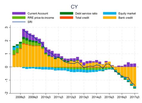
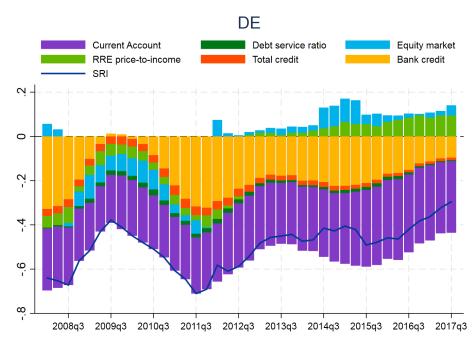
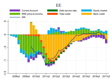
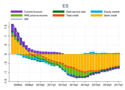
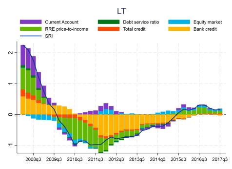
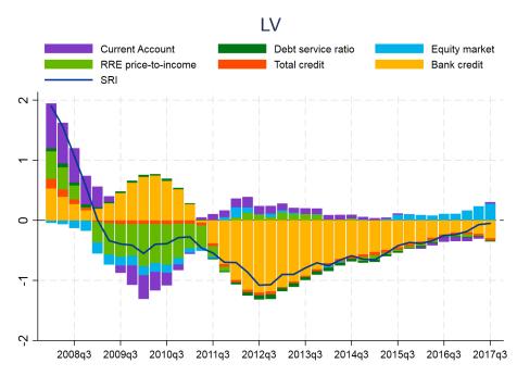
64 Chart A.7 A.6 Decompositions of the benchmark d-sri Benchmark d-sri for all euro area countries and decomposition into underlying driving factors (horizontal axis: date; vertical axis: benchmark d-sri and contributions by different d-sri components) ECB Occasional Paper Series No 219 / February

65 Source: ECB calculations based on various data sources. Notes: The benchmark d-sri is constructed as a weighted average of the normalised sub-indicators; normalisation is performed by subtracting the median and dividing by the standard deviation of the pooled indicator distribution across countries and time. See Table 2 for details. ECB Occasional Paper Series No 219 / February

66 A.7 Robustness of d-sri dynamics and early warning properties Charts A.8 and A.9 show that there is a high correlation between the early warning performance of the individual indicators when computed for the euro area countries and when computed for the euro area countries plus Denmark, Sweden and the United Kingdom. Adding Denmark, Sweden, and the United Kingdom to the analysis therefore increases the number of observations and crisis events (especially for the earlier part of the sample) without altering the results materially. Chart A.8 Adding DK, SE and the United Kingdom to the euro area (EA) countries increases observations, but does not alter the analysis Comparison of AUROC values for EA countries and EA countries plus DK, SE, and UK (x-axis: AUROC on EA only; AUROC on EA, DK, SE and UK) Sources: ECB calculations based on the ECB/ESRB financial crises database. Notes: The yellow line is the 45-degree line. AUROC is computed for a pre-crisis horizon of 12-5 quarters. The dating of systemic financial crises is based on the ECB/ESRB crises database described in Lo Duca et al. (2017). Purely foreign induced crises are excluded. Variables labelled are the ones with the highest distance from the 45-degree line (top and bottom 5th percentile). ECB Occasional Paper Series No 219 / February

67 Chart A.9 Adding DK, SE and UK to the EA countries increases observations, but does not alter the analysis Relative usefulness out-of-sample computed on the whole sample and only for the EA (x-axis: Relative usefulness on EA only; y-axis: Relative usefulness on EA, DK, SE and UK) Sources: ECB calculations based on the ECB/ESRB financial crises database. Notes: The yellow line is the 45-degree line. Out-of-sample early warning properties are evaluated with the relative usefulness for balanced preferences based on a recursive quasi real-time exercise for the pre-crisis period 12-5 bench that starts in Q The dating of systemic financial crises is based on the ECB/ESRB crises database described in Lo Duca et al. (2017). Purely foreign induced crises are excluded. Variables labelled are the ones with the highest distance from the 45-degree line (top and bottom 5th percentile). Variables that have very poor relative usefulness (negative) are omitted. The early warning performance of the benchmark d-sri is robust to various perturbations and it performs considerably better in real-time than a d-sri based on country-specific normalisation. In order to gauge the robustness of the signals from the benchmark d-sri, various alternative d-sri specifications with different indicator normalisations and indicator weights are constructed. First, three versions of the d-sri are constructed with re-optimised weights, where equity prices ( d-sri excl. equity ), RRE prices ( d-sri excl. RRE ) and the current account balance ( d-sri excl. CA bal ) are excluded respectively. This helps to gauge the robustness of the benchmark d-sri to excluding specific risk drivers. Second, three different optimal weighting schemes are derived based on alternative definitions of the vulnerability periods. d-sri (all crises) adds systemic crises that are purely due to foreign factors to the benchmark crises definition and uses the same pre-crisis horizon of 12-5 quarters to obtain optimal weights. d-sri (20-5q) uses the benchmark crises with a longer pre-crisis horizon of 20-5 quarters to optimise weights, while d-sri (ESRB crises) uses the crises definition from Detken et al. (2014) with a 12-5 quarter pre-crisis horizon. Third, three different optimal d-sri weighting schemes are produced based on shorter historic data samples. d-sri (1995q1), d-sri (2002q1) and d-sri (2010q1) only use data up to 1995q1, 2002q1, and 2010q1 respectively to estimate the optimal d-sri weights. Fourth, a version of the d-sri with new optimal ECB Occasional Paper Series No 219 / February

68 weights is created where the normalisation of d-sri sub-indicators is performed based on full-sample country-specific moments ( d-sri country ). Fifth, quasi-real time versions of the benchmark and country-specific d-sris are constructed ( d-sri RT and d-sri country RT ) that use recursively computed values of the median and standard deviation for normalisation instead of full sample values. Charts A.10 to A.12 and Table A.11 show that the early warning performance, the d-sri weights and the d-sri dynamics appear rather robust to many of these robustness exercises. Chart A.10 The performance of the benchmark d-sri is robust to various perturbations and it performs considerably better in quasi real-time than a d-sri with country-specific indicator normalisation AUROC values for different versions of the d-sri (x-axis: d-sri version; y-axis: AUROC) Benchmark SRI SRI RT SRI country SRI country RT SRI excl. RRE SRI excl. Equity SRI excl. CA bal SRI (20-5q) SRI (All crises) SRI (ESRB crises) SRI (1995q1) SRI (2002q1) SRI (2010q1) Source: ECB calculations based on the ECB/ESRB EU financial crises database. Notes: The set of financial crises to compute the early warning performance comprises all systemic financial crises episodes from the new ECB/ESRB EU financial crises database that are not purely due to foreign factors (see Lo Duca et al. (2017) for details). The relevant vulnerability periods are defined as 12-5 quarters prior to the systemic financial crises of interest. The benchmark d-sri is constructed as a weighted average of the normalised sub-indicators, where the normalisation is performed by subtracting the median and dividing by the standard deviation of the pooled indicator distribution across countries and time. The six underlying indicators of the d-sri are as follows (indicator weights are indicated in brackets): the 2-year change in the bank credit-to-gdp ratio (0.36), the 2-year growth rate of real total credit (0.05), the 2-year change in the debt-service-ratio (0.05), the 3-year change in the residential real estate price-to-income ratio (0.17), the 3-year growth rate of real equity prices (0.17), and the current account-to-gdp ratio (0.20). Different versions of the d-sri, where optimal weights are re-computed every time, are displayed to gauge robustness of the results. RT indicates that the median and standard deviation for normalisation are computed recursively (in quasi real-time). Country indicates that the median and standard deviation for normalisation are computed separately for each country. The d-sris with excl. show versions where one of the components is excluded from the d-sri (and weights are re-optimised for the other remaining variables). CA bal is the current account balance, RRE is the house price to income ratio. All crises adds the systemic crises that are purely due to foreign factors to the benchmark crises definition and uses the same pre-crisis horizon of 12-5 quarters to obtain new optimal weights. ESRB crises uses the crisis definition from Detken et al. (2014), with a 12-5 quarter pre-crisis horizon. 20-5q uses the benchmark crises with a longer pre-crisis horizon of 20-5 quarters to optimise weights. Dates indicated in brackets describe the data sample that is used to obtain optimal weights, i.e. 1995q1 implies that only data up to 1995q1 is used to obtain optimal d-sri weights. ECB Occasional Paper Series No 219 / February

69 Table A.11 The optimal weights from the benchmark d-sri are rather robust to a number of perturbations Optimal indicator weights for different versions of the d-sri 2-year change in the bank credit-to-gdp ratio 2-year growth rate of real total credit 3-year change in RRE price-to-income ratio 3-year growth rate of real equity prices 2-year change in the debt-service-ratio Current accountto-gdp ratio Benchmark d-sri d-sri real-time d-sri country d-sri country real-time d-sri excl. RRE d-sri excl. equity d-sri excl. CA bal d-sri (20-5q) d-sri (all crises) d-sri (ESRB crises) d-sri (data until 1995q1) d-sri (data until 2002q1) d-sri (data until 2010q1) Source: ECB calculations based on the ECB/ESRB EU financial crises database. Notes: The set of financial crises to compute the optimal indicator weights comprises all systemic financial crises episodes from the new ECB/ESRB EU financial crises database that are not purely due to foreign factors (see Lo Duca et al. (2017) for details). The relevant vulnerability periods are defined as 12-5 quarters prior to the systemic financial crises of interest. The benchmark d-sri is constructed as a weighted average of the normalised sub-indicators, where the normalisation is performed by subtracting the median and dividing by the standard deviation of the pooled indicator distribution across countries and time. The six underlying indicators of the d-sri are as follows (indicator weights are indicated in brackets): the 2-year change in the bank credit-to-gdp ratio (0.36), the 2-year growth rate of real total credit (0.05), the 2-year change in the debt-service-ratio (0.05), the 3-year change in the residential real estate price-to-income ratio (0.17), the 3-year growth rate of real equity prices (0.17), and the current account-to-gdp ratio (0.20). Different versions of the d-sri, where optimal weights are re-computed every time, are displayed to gauge robustness of the results. RT indicates that the median and standard deviation for normalisation are computed recursively (in quasi real-time). Country indicates that the median and standard deviation for indicator normalisation are computed separately for each country. The d-sris with excl. show versions where one of the components is excluded from the d-sri (and weights are re-optimised for the other remaining variables). CA bal is the current account balance, RRE is the house price to income ratio. All crises adds the systemic crises that are purely due to foreign factors to the benchmark crises definition and uses the same pre-crisis horizon of 12-5 quarters to obtain new optimal weights. ESRB crises uses the crisis definition from Detken et al. (2014), with a 12-5 quarter pre-crisis horizon. 20-5q uses the benchmark crises definition with a longer pre-crisis horizon of 20-5 quarters to optimise weights. Dates indicated in brackets describe the data sample that is used to obtain optimal weights, i.e. 1995q1 implies that only data available up to 1995q1 is used to obtain optimal d-sri weights. Weights sometimes do not sum to 1 due to rounding. ECB Occasional Paper Series No 219 / February

70 Chart A.11 Dynamics of the benchmark d-sri and supplementary d-sri versions excluding some sub-indicators (horizontal axis: date; vertical axis: benchmark d-sri and supplementary d-sri versions) ECB Occasional Paper Series No 219 / February

71 Source: ECB calculations based on various data sources. Notes: The black shaded areas indicate systemic financial crises episodes from the new ECB/ESRB EU financial crises database that are not purely due to foreign factors (see Lo Duca et al. (2017) for details). The grey shaded areas indicate vulnerability periods that are defined as 12-5 quarters prior to the systemic financial crises of interest. The blue shaded areas indicate other relevant events that encompass systemic financial crises that are purely due to foreign factors according to the ECB/ESRB EU database and residual financial stress events that were relevant from a macroprudential perspective. The benchmark d-sri is constructed as a weighted average of the normalised sub-indicators. Normalisation is performed by subtracting the median and dividing by the standard deviation of the pooled indicator distribution across countries and time. The two supplementary d-sri versions exclude the equity price and current account indicators respectively, and weights are re-optimised for the remaining d-sri components. ECB Occasional Paper Series No 219 / February

72 Chart A.12 Dynamics of the benchmark d-sri and d-sri versions based on quasi real-time information (horizontal axis: date; vertical axis: benchmark d-sri and supplementary d-sri versions) ECB Occasional Paper Series No 219 / February

73 Source: ECB calculations based on various data sources. Notes: The black shaded areas indicate systemic financial crises episodes from the new ECB/ESRB EU financial crises database that are not purely due to foreign factors (see Lo Duca et al. (2017) for details). The grey shaded areas indicate vulnerability periods that are defined as 12-5 quarters prior to the systemic financial crises of interest. The blue shaded areas indicate other relevant events that encompass systemic financial crises that are purely due to foreign factors and residual financial stress events that were relevant from a macroprudential perspective. The benchmark d-sri is constructed as a weighted average of the normalised sub-indicators. Normalisation is performed by subtracting the median and dividing by the standard deviation of the pooled indicator distribution across countries and time. The two supplementary d-sri versions use optimal weights estimated based on data available in 1995 and weights that are re-optimised when using sub-indicators that are normalised based on quasi real-time recursive data moments rather than based on full-sample data moments. ECB Occasional Paper Series No 219 / February

74 A.8 Details on local projections and quantile regressions We estimate local projection impulse response functions as proposed by Jordà (2005) as these are more robust to possible model misspecification than impulse responses from a VAR. Let xx ii,tt be the d-sri and yy ii,tt the one-year ahead real GDP growth rate in country ii at time tt. Let h > 0 be the prediction horizon and denote aa h = aa 0,h, aa 1,h,, aa PP,h, bb h = bb 0,h, bb 1,h,, bb PP,h, YY ii,tt = yy ii,tt, yy ii,tt 1,, yy ii,tt PP,XX ii,tt = xx ii,tt, xx ii,tt 1,, xx ii,tt PP The baseline specification for the estimation of the local projection impulse response function controlling for country fixed effects is: yy ii,tt+h = γγ h,ii + aa h YY ii,tt + bb h XX ii,tt + ee h,ii,tt where the coefficient bb 0,h is interpreted as the response of one-year ahead real GDP growth to a unit impulse of the d-sri at horizon h. This impulse response averages across large declines in economic activity, economic boom periods as well as episodes of normal economic growth. In order to isolate the predictive power of the d-sri for the left tail of the conditional GDP growth distribution, we resort to quantile regression estimation. Let τ (0,1) and denote aa h (τ) = aa 0,h (τ), aa 1,h (τ),, aa PP,h (τ), bb h = bb 0,h (τ), bb 1,h (τ),, bb PP,h (τ), YY ii,tt = yy ii,tt, yy ii,tt 1,, yy ii,tt PP,XXii,tt = xx ii,tt, xx ii,tt 1,, xx ii,tt PP The baseline specification for quantile regression estimation is: yy ii,tt+h (τ) = γγ h,ii (ττ) + aa h (τ)yy ii,tt + bb h (τ)xx ii,tt + ee h,ii,tt (τ) where the coefficient bb 0,h (τ) is interpreted as the response of the τ-th conditional quantile of one-year ahead GDP growth to a unit impulse of the d-sri at horizon h. The sample for estimating the local projections and quantile regressions encompasses all available data for the euro area countries, plus Denmark, Sweden and the United Kingdom from Q to Q The baseline specifications control for ten lags of one-year ahead real GDP growth and ten lags of the d-sri, as well as country fixed effects. ECB Occasional Paper Series No 219 / February

75 A.9 Robustness of d-sri impulse response functions Chart A.13 Response of average real GDP growth to a d-sri impulse of one standard deviation size The three charts show robustness of Chart 18 to (1) dataset confined up to Q1 2006, (2) dataset confined to large countries (DE, IT, FR, ES, NL), (3) using 3 lags instead of 10. (horizontal axis: horizon in quarters; vertical axis: one-year ahead GDP growth) Source: ECB calculations based on various data sources. ECB Occasional Paper Series No 219 / February