4. Introduction to Prescriptive Analytics. BIA 674 Supply Chain Analytics

Transcription

1 4. Introduction to Prescriptive Analytics BIA 674 Supply Chain Analytics

2 Why is Decision Making difficult? The biggest sources of difficulty for decision making: Uncertainty Complexity of Environment or of System Difficulty of Measuring or even Studying alternative Strategies Do NOT procrastinate! Do NOT hide your head under the sand! Do NOT ignore data & evidence!

3 Simple pieces for advice Overcome your anxieties Let go your inner perfectionist Maintain a balance between Analysis/deliberation and action Data gathering and obtaining of results Alternative goals (that might even be conflicting) remember: balanced scorecard Quantitative vs. qualitative approaches Manage Meetings (Group decision making) Hidden agendas, fights, late starts, topic switching, Create Shared Understanding Try for Consensus at least about the problem

4 Can we avoid wrong decisions? There is NO such thing as a perfect decision maker. Even with all the supercomputers in the world, you will STILL make mistakes Difference between WRONG vs. BAD decision: You cannot avoid some bad decisions, but TRY to avoid the bad ones! Difference between outcomes and process! What are the key decision TRAPS? Control the process

5 Rule 1: Avoid the decision traps Status Quo trap Anchoring trap Confirming evidence trap And more How do you avoid decision traps?

6 Rule 2: Follow the rational process Problem Identification System Analysis Goal Formulation Initial System Design Implement Solution Solution Analysis Model Solution Model Formulation The importance of analytics & modeling!

7 Solving the right problem Better have an approximate solution to today s problem than an optimal solution to yesterday s problem Make sure you get problem statement right Objective (often multiple conflicting objectives) Constraints (often too many) Test with a known solution Data Quality is key Garbage in, garbage out Make sure you always output a solution Relax the problem, move constraints to objective Handle the computational time Trade offs among solution quality vs feasibility vs optimality

8 Basic concepts & decision models Prescriptive Decision Models help decision makers identify the best solution: Optimization - finding values of decision variables that minimize (or maximize) something such as cost (or profit). Decision Variables - the variables whose values the decision maker is allowed to choose. Objective function - the equation that minimizes (or maximizes) the quantity of interest. Constraints - limitations or restrictions that must be satisfied.

9 Basic concepts & decision models Feasible solution - is any set of values of the decision variables that satisfies all of the constraints. Feasible region - the set of all feasible solutions. Infeasible solution - is a solution where at least one constraint is not satisfied. Optimal solution - values of the decision variables at the minimum (or maximum) point that satisfy some necessary optimality conditions Global and local optimality A local optimum is a solution that is optimal within a neighboring set of solutions. Global optimum is the optimal solution among all possible solutions

10 Evolution & Quality of Information Depending on the Quality of Information: Deterministic models have inputs that are known with certainty. Stochastic models have one or more inputs that are not known with certainty. Depending on the Evolution of Information: Static models where all inputs are known in advanced (with certainty or uncertainty). Dynamic models where input data is revealed in real time during the planning horizon.

11 Types of Deterministic Models Linear versus Nonlinear (convex optimization) Linear/nonlinear functions for objective and/or constraints (LP / NLP) Discrete versus Continuous Continuous, integer, binary and/or mixed integer decision variables (ILP / IP/ MIP / MILP / MINLP) Convex versus non Convex Quadratic Programming (QP / MIQP) Unconstrained: No constraints Dynamic Programming: Solved in stages Combinatorial Optimization

12 Optimization Methods Algorithms are systematic procedures used to find optimal solutions to decision models. Exact Mathematical Programming algorithms provide guarantee for finding the (global) optimum Simplex, Interior Point (Barrier), Complete Enumeration, Branch and Bound/Cut/Price, Gradient Methods Heuristic algorithms trade optimality for efficiency and they are used to find high quality solutions in a reasonable amount of time. Construction heuristics, Local Search, Evolutionary and Genetic Algorithms, Swarm Intelligence

13 A simple problem for you You start working tomorrow as a Production Manager in a Manufacturing Company: Producing 50 different products (or variations) Out of 15 resources (raw materials, machine -hours, man - hours by speciality,...) All 50 products PROFITABLE! Whatever quantity we make of each product (within our capacities) can be sold (we are small compared to the size of the market) Our ONLY criterion (to start with) is PROFITABILITY (i.e. no market share,...)

14 Question: How many out of the 50 products would you consider reasonable to produce? All 50? 40? 30? 15? 5? 1? Do you need more info to answer? WHY?

15 Why? Consider a simple case 1 15 A company is producing 50 products out of 1 resource Product P i requires Q i units of the resource to be produced 1 unit of product P i generates revenue R i Products Q Q 1 Q 2 Q 50 R R 1 R 2 R 50

16 How many products to produce? Assume that all production can be sold! Our objective is to max revenue! Best strategy is to produce the ONE product that maximizes the ratio: R i / Q i (REMEMBER: BEST VALUE FOR MONEY)

17 Extension To two resources Generally KEY CONCLUSIONS Do NOT spread yourself too thin! Put your resources where they will generate the most output! This is a result of the Linearity assumption Use as a YARDSTICK!

18 Generally, Optimization helps businesses make complex decisions and trade-offs about limited resources Discover previously unknown options or approaches Automate and streamline decisions Compliance with business policies and regulations Explore more scenarios and alternatives Understand trade-offs and sensitivities to various changes Gain insights into input data View results in new ways

19 Introduction to Linear Programming Optimization

20 An Example 1 20 Manufacturing company Producing 2 products: P1 & P2 Out of 3 raw materials: A, B, C Products sell for 200 & 300 euros per unit Company has available stock for 30, 20 and 36 units Bill-of-materials: Raw Material P1 Products P2 Available Stock A B C Price Question: What is the best production plan? (i.e. maximizing revenue)

21 Try alternative solutions? 1 21 P 1 =20 P 2 =20? P 1 =20 P 2 =10? P 1 =10 P 2 =20? P 1 =15 P 2 =5? P 1 =5 P 2 =15? P 1 =5 P 2 =12? Raw Material Products Available Stock P1 P2 A B C Price Questions: Are the above plans feasible? If feasible, are they the best?

22 Formulation of a model (3 steps) 1 22 A. Determine decision variables x 1 = production quantity of P1 x 2 = production quantity of P2 B. Determine objective : MAX REVENUE (Z) Z = 200x x 2 C. Determine constraints (Limited Resources) Limited A x 1 +2x 2 30 Limited B x 1 + x 2 20 Limited C 2x 1 + x 2 36 x 1, x 2 0

23 Graphical representation of a constraint x 2 10 x 1 + 2x 2 = 30 (A) x 1

24 Graphical Analysis of Constraints 1 24 x x 1 + x 2 = 20 (B) x 2 x x 1 + x 2 = 36 (C) x 1

25 Putting all constraints together 1 25 x A Obviously, the production plan to be selected must satisfy all the constraints. 20 B C x 1

26 The FEASIBLE region 1 26 X 2 15 II FEASIBLE REGION 10 III 5 I IV V 20 X 1 1. All points within the shaded area satisfy the constraints with Inequality, i.e. leave slack resources! 2. All points on the boundaries (except the corner points) utilize one resource completely, but leave slack resources of the other two! 3. The corner points III and IV utilize two resources fully!

27 Getting to the optimal plan 1 27 X 2 x 2 Z=1200 Z=200x x 2 III Z=600 Z* X 1 x 1 Therefore, the OPTIMAL PRODUCTION is given by point III which is the intersection of constraints (A) & (B)! At this CORNER POINT, resources (A) & (B) are FULLY UTILIZED, whereas resource (C) is not! To determine point III, solve A & B as equalities, simultaneously: x 1 + 2x 2 = 30 x 1 + x 2 = 20 x 1* = x 2* = 10 ; Z * = 5,000

28 Sensitivity Analysis 1 28 What happens if the prices of two products change? Assume the objective function is: Z = c 1 x 1 + c 2 x 2 (with c 1 = 200, c 2 = 300) By changing the prices c 1 and c 2, the slope, of the objective function changes: For small variations, same optimum remains! For large variations, the optimum moves to a neighboring corner The critical factor is not the values of the prices, but their relative ratio

29 Sensitivity Analysis 1 29 Specifically: If...c 1 /c 2 ½...optimal is II If...½ c 1 /c optimal is III If... 1 c 1 /c optimal is IV If... 2 c 1 /c optimal is V NOTE: 1. Optimal point is ALWAYS A CORNER POINT! 2. Even if price of P1 (c 1 ) increases by 30%, WE DO NOT produce more of P1!!! 3. When the price of P1 exceeds that of P2 (i.e. c 1 /c 2 1), only then do we change the production plan, and we change it drastically. The new production plan will be at corner IV [utilizing (B) and (C) with x 1 = 16 and x 2 = 4!!!

30 Sensitivity Analysis 1 30 What happens if the availabilities of the resources change? Assume that availability of A becomes 29 instead of 30 How do you expect the strategy to change? How do you expect the bottom line to change? By changing the prices b A the feasible region decreases! Even for small variations of the critical resources, the strategy changes! So does the bottom line! This is radically different from the previous result (prices)!

31 General Formulation of LP Problems Determine the values (x 1, x 2,..., x n ) for activities (1, 2,..., n) so as to: Max Z = c 1 x 1 + c 2 x c n x n subject to: a 11 x 1 + a 12 x a 1n x n b 1 a 21 x 1 + a 22 x a 2n x n b 2 a m1 x 1 + a m2 x a mn x n b m x 1, x 2,..., x n 0 Variations of the Above Standard Form Minimization objective Constraints of the form, or Constraints of the form = Variables x j 0, or Variables x j without constraint

32 Assumptions of Linear Programming 1. LINEARITY 2. DIVISIBILITY 3. CERTAINTY

33 Linearity 1 33 Linear graph vs. non-linear graph Proportionality of output to the input Examples of linear relationships production of products vs. time transportation costs vs. weight (usually) distance traveled vs. time (with const. speed) Examples of non-linear relationships Economics of scale The typist example transportation costs with economies or discounts Examples of piecewise linear relationships approximations to non-linear relationships

34 Linear Relation Input - Output Always remember: The change in the output for a given change of input is constant at every value of the input x 1 y Δx 1 Δy x x Example: y = 20-4x 1 +2x x x x x 2 1-4

35 Divisibility 1 35 Activities can take any value, i.e. not necessarily integers Examples: hours of operation of a machine gallons of petrol pounds of wheat budget, etc. Integer variables: no. of branches of a bank no. of employees no. of books printed, etc. In this case use INTEGER PROGRAMMING. Note: Even then, approximation using LP is possible if the values are big! In this case... round-off to the nearest integer. Approximation is not possible for 0/1 problems!!!

36 Certainty 1 36 All parameters of the problem are known, i.e. Constraints in the objective function (prices) RHS (availabilities) Constants of the matrix (specifications of production) Note: Even if not known, we can do a Sensitivity Analysis!

37 Optimization Overview Variables: x ( x, x,..., x 1 2 N ) Objective: min f ( x) Subject to Functional and Regional Equations and Constraints: Sometimes additional constraints: Binary Integer Sometimes uncertainty in parameters (stochastic optimization) x X g( x) b h( x) k...

38 Example: Asset & Liability Management Loans short-term (12%) medium-term (10%) long-term (8%) Stocks average return (15%) Oblig. deposits at the Central Bank interest = 4% Cash Current Accounts total available = $10bn Deposit Accounts total available = $45 bn Deposits: time deposits total available =$45 bn

39 Special considerations a) Liquidity: 5%, 3% and 1% of available for each category of deposits b) Loans Limitations: short-term between 10% and 15% of total deposits long-term between 15% and 20% of total deposits c) Obligatory Deposits (to the Central Bank): at least 8% of total deposits Determine the optimal structure of the Bank s assets (to max total Return on Assets)

40 The model Let x i = % of total deposits placed in asset i i = 1 short term loans i = 2 medium-term loans i = 3 long-term loans i = 4 stocks i= 5 obligatory placements i = 6 cash Max Z = 0.12x x x x x 5 s.t x x x x 6 [(0.05)(10)+(0.03)(45)+(0.01)(45)]/100 = (=1.85%) x 1 + x x 6 = 1 x i 0 i = 1, 2,..., 6

41 Basic economic concepts Duality

42 Example: The diet problem A Consumer s diet should include daily at least 9 vitamins A and 19 vitamins C. The Consumer visits the local supermarket and determines 6 foods (F1,..., F6) that include these vitamins, as follows: Vitamins Contents per 100 gm F1 F2 F3 F4 F5 F6 A C Price / 100 gm Assuming that he has no preference among the 6 foods, his problem is to select the MINIMUM COST

43 The model Mathematical Model Determine (x 1, x 2,..., x 6 ) = quantities of foods to buy MIN Z = 35x x x x x x 6 s.t. x 1 + 2x 3 + 2x 4 + x 5 + 2x 6 9 x 2 + 3x 3 + x 4 + 3x 5 + 2x 6 19 x 1,..., x 6 0 Solution x 5 = 5, x 6 =2, x 1 =... = x 4 = 0 Z = 169

44 Some questions 1. Why not buy any of the other foods? 2. What would it take to buy them? 3. What happens if the doctor changes the prescription? 4. What is competition, and what would competition do? Vitamins Contents per 100 gm F1 F2 F3 F4 F5 F6 A C Price / 100 gm

45 The competition 1 45 The pharmacist What is his/her objective? What are his/her constraints? Determine prices P A and P C for the vitamins, so that he/she maximizes his/her revenue while staying competitive! Can we formulate an LP to solve it?

46 The model 1 46 Determine (P A, P C ) = prices of vitamins A, C MAX = 9P A + 19P C s.t. P A 35 (F 1 ) P C 30 (F 2 ) 2P A + 3P C 60 (F 3 ) 2P A + P C 50 (F 4 ) P A + 3P C 25 (F 5 ) 2P A + 2P C 22 (F 6 ) P A, P C 0

47 The solution 1 47 P A = 4.. Dual Price of vitamin A P C = 7.. Dual Price of vitamin C Θ = Max Revenue Can you explain this? What is the meaning of these dual prices? What do they mean to the customer s budget? What are the surplus costs?

48 Dual Prices and Surplus Costs 1 48 Dual prices give us the change in the objective function value if the RHS changes by 1 unit! For how long is this dual price valid? Is the dual price increasing or decreasing as we increase the RHS (availability)? Why? Surplus cost gives us the change that has to occur to a non-basic variable to become basic! Remember: if x>0 then Surplus cost = 0, AND x = 0 then Surplus cost > 0 Can you explain? Is it clear how many basic variables we will have? Sensitivity analysis gives us the range of values in the RHS (or in the objective function) where the strategy (or the dual prices remain constant. if

49 1 49 The charcoal example

50 Three important managerial questions 1 50 Suppose next week the doctor changes the prescription from 9 A s and 19 C s to 10 A s and 19 C s. Will this change the budget of the consumer? If so, by how much? By how much should the supermarket lower the prices of the vitamins not sold, in order to make them attractive? Suppose there is a new food with 3 A s, and 5 C s which should sell at 59c. Should the supermarket get this new food?

51 Dual Prices 1 51 The dual price of a resource is: Internal Value of this resource! How much it is worth to us! How much the objective function would increase if we had 1 more unit available! The dual price depends: On the availability of this resource On the efficiency of our technology On the brand name and the prices of our finished products Dual prices of the same resource are different across users, and the dual price is different from its price

52 The Dual Price = The Real Value 1 52 It is very important to know the dual price of a resource: We know how much and at what price we should buy them in the market We determine our really valuable resources We identify good opportunities to buy We can price-out new products or activities and calculate their profitability Of course, we can also price-out existing products or activities Example: a new food appears with 4A s and 2C s, costing 47c would the customer prefer it? REMEMBER: A DUAL PRICE FOR EVERY CONSTRAINT!

53 Surplus Cost 1 53 The surplus cost of a variable is the change required in the price of this product to make it competitive in the market! to start buying it! to raise its activity level to zero! to make this variable BASIC! A Surplus cost exists ONLY if the variable is zero! Otherwise, its activity level is already positive!

54 Surplus Cost = Extra Cost 1 54 It is connected to the dual price We can validate the surplus cost of an activity or a product by calculating the difference Surplus Cost = = Price of a product Priced-out sum of values of its resources It is very important we know the surplus costs of our products this way we will know: How much we can reduce prices! Which are the hopeless products! How we compare with competition! and, what happens if competition s prices are lower, even after the reduction of surplus cost?

55 Remember 1 55 Every constraint is associated with a DUAL PRICE Try to understand what it means for every constraint Can the dual price be zero? When? Every variable is associated with a SURPLUS COST Try to understand what it means for every variable Can the surplus cost be zero? When? Dual prices and surplus costs ARE RELATED though pricing out Dual prices and Surplus costs can be read out of the SOLVER output

56 Sensitivity Analysis for LPs An excellent way to address UNCERTAINTY using LP Often it is useful to perform sensitivity analysis to see how (or if) the optimal solution changes as one or more inputs change. The Solve dialog box offers you the option to obtain a sensitivity report. Solver s sensitivity report performs two types of sensitivity analysis: 1. on the coefficients of the objectives, the c s, and 2. on the right hand sides of the constraints, the b s.

57 Refinery Example: A Transportation problem 1 57 Oil is to be transported from 4 refineries (A, B, C, D) to 3 depots (1, 2, 3) The availability in each refinery (in tanker loads) is: 22, 41, 27, 10 The demand to be satisfied at every depot (in tanker loads) is: 30, 45, 14 Depots A B C D

58 From the SOLVER output 1 58 Target Cell (Min) Cell Name Original Value Final Value $E$9 Cost Adjustable Cells Cell Name Original Value Final Value $B$5 Refinery 1 Depot $C$5 Refinery 1 Depot $D$5 Refinery 1 Depot $B$6 Refinery 2 Depot $C$6 Refinery 2 Depot $D$6 Refinery 2 Depot $B$7 Refinery 3 Depot $C$7 Refinery 3 Depot $D$7 Refinery 3 Depot $B$8 Refinery 4 Depot $C$8 Refinery 4 Depot $D$8 Refinery 4 Depot Constraints Cell Name Cell Value Formula Status Slack $F$12 Availability of refinery 1 Used $F$12<=$G$12 Binding 0 $F$13 Availability of refinery 2 Used $F$13<=$G$13 Not Binding 10 $F$14 Availability of refinery 3 Used $F$14<=$G$14 Binding 0 $F$15 Availability of refinery 4 Used $F$15<=$G$15 Binding 0 $F$16 Requirements of depot 1 Used $F$16=$G$16 Not Binding 0 $F$17 Requirements of depot 2 Used $F$17=$G$17 Not Binding 0 $F$18 Requirements of depot 3 Used $F$18=$G$18 Not Binding 0 $B$5 Refinery 1 Depot $B$5>=0 Binding 0.00 $C$5 Refinery 1 Depot $C$5>=0 Not Binding $D$5 Refinery 1 Depot $D$5>=0 Binding 0.00 $B$6 Refinery 2 Depot $B$6>=0 Not Binding 3.00 $C$6 Refinery 2 Depot $C$6>=0 Not Binding $D$6 Refinery 2 Depot $D$6>=0 Not Binding 5.00 $B$7 Refinery 3 Depot $B$7>=0 Not Binding $C$7 Refinery 3 Depot $C$7>=0 Binding 0.00 $D$7 Refinery 3 Depot $D$7>=0 Binding 0.00 $B$8 Refinery 4 Depot $B$8>=0 Binding 0.00 $C$8 Refinery 4 Depot $C$8>=0 Binding 0.00 Optimal Solution: X12 = 22 X21 = 3 X22 = 23 X23 = 5 X31 = 27 X43 = 10 Z = 3,780 Why not use route 13? Would total cost change if refinery 4 had 1 more tanker load available?

59 From the SOLVER output 1 59 Adjustable Cells Final Reduced Objective Allowable Allowable Cell Name Value Cost Coefficient Increase Decrease $B$5 Refinery 1 Depot E $C$5 Refinery 1 Depot E+30 $D$5 Refinery 1 Depot E $B$6 Refinery 2 Depot $C$6 Refinery 2 Depot $D$6 Refinery 2 Depot $B$7 Refinery 3 Depot E+30 $C$7 Refinery 3 Depot E $D$7 Refinery 3 Depot E+30 0 $B$8 Refinery 4 Depot E $C$8 Refinery 4 Depot E $D$8 Refinery 4 Depot E+30 Constraints Final Shadow Constraint Allowable Allowable Cell Name Value Price R.H. Side Increase Decrease $F$12 Availability of refinery 1 Used $F$13 Availability of refinery 2 Used E $F$14 Availability of refinery 3 Used $F$15 Availability of refinery 4 Used $F$16 Requirements of depot 1 Used $F$17 Requirements of depot 2 Used $F$18 Requirements of depot 3 Used From dual prices/reduced costs Cost of route 13 has to be reduced by 60! If R4 s availability increases by 1, then the total cost goes down by 60! VERIFY IT!

60 Modelling Mixed Integer Linear Problems

61 Integer Programming Problems Allocation of workers per shift Production of cars per week Number of bank branches operating in an area All problems of allocation of resources, when some or all of these resources or activities can be allocated or undertaken at integer values. Usually, these problems can be approximated using Linear Programming, and rounding-off to the nearest integer ONE exception

62 Binary Problems 1 62 A special category of Integer Problems The variables take only the values 0 or 1 (binary variable) These are logical variables not physical variables They represent logical decisions (YES/NO), not physical quantities They cannot be solved sing LP no rounding off can occur! They need special art in the formulation They appear very frequently in many problems: Investment evaluation and selection Distribution and vehicle routing Production scheduling

63 Example: The Knapsack Problem Assume you are going for a 3-day safari. Your knapsack can take items of total weight no more than 20 Kilos and total volume no more than 30 gallons You are asked to choose among 10 items (foods), each one being characterised by a weight w i, a volume v i, and a value c i,. Your objective is to choose the best combination among the 10 items available, i.e. the ones that maximize the total value of your knapsack.

64 Knapsack problem: Solution Let X i = 1, if item i (i = 1 10) is to be included in the knapsack 0, otherwise Problem Formulation: Max Z = c 1 X 1 + c 2 X c 10 X 10 s.t. w 1 X 1 + w 2 X w 10 X v 1 X 1 + v 2 X v 10 X X 1,..., X 10 = 0/1

65 Variations around Knapsack problem 1. Assume that items1 and 2 are competitive, i.e. there is no sense in bringing both of them, since you will be consuming only one, (e.g. two types of toothpaste). X 1 + X Assume that items 3 and 4 are complementary, i.e. if you take one with you, you also have to take the other as well, and vice versa (e.g. pasta and tomato sauce). X 3 = X 4 3. Assume that foods 5 and 6 are partially complementary, i.e. if you take the first (e.g. coffee), you also have to take the second (e.g. milk). This in not true the other way. X 5 X 6 Note: The above is an investment selection problem

66 Case 1: Investment Selection You are considering how to best allocate the $4 M available to the following investments that receive some subsidy: INVESTMENT COST (million $) RETURN (million $) 1 Casino in Rhodes Casino in Corfu Private Airport in Corfu Casino in North Evia Factory in North Evia 1, Housing in North Evia Cost = Own funds (over and above the subsidy)

67 Case 1: Investment Selection By law, the government can only acquire a licence for 1 casino. If the casino in Corfu is selected, then a small private airport needs to also be built (because no good transportation currently exists). The airport in Corfu is certainly beneficial anyway. A casino can not be operated in an industrial area. If the factory in Evia is constructed, the housing need for the workers must also be taken care of. But if the factory in Evia is not constructed, the houses do not need to be constructed either. Total budget (own funds) restricted to $4 million.

68 Case 1: The Model Let x i = 1 if you undertake investment i = 0 otherwise Max Z = 4.20x x x x x x 6 s.t. 2.50x x x x x x 6 4 x 1 + x 2 + x 4 1 x 2 x 3 x 4 + x 5 1 x 5 = x 6 x i = 0/1

69 Case 2: Distribution Four trucks are available to deliver milk to five grocery stores. The demand of each grocery store can be supplied by only truck, but a truck may deliver to more than one grocery. Truck Capacity (gallons) Daily Operating Cost ($) Daily Demand Grocery (gallons) Determine how to minimize the daily cost of meeting the demands of the five groceries. 69

70 Case 2: Distribution Let Y i = Let X ij = so that 1, if truck i (i = 1 4) operates on a particular day to deliver milk 0, otherwise 1, if truck i (i = 1..4) is used to deliver milk to grocery store j (j = 1,, 5) 0, otherwise min Z 45Y 1 50Y2 55Y3 60 Y 4 Truck 1 Capacity: Problem Formulation: Truck 2 Capacity: Truck 3 Capacity: Truck 4 Capacity: 100 X Y X X X X X Y X X X X X Y X X X X X Y X X X X X 1j + X 2 j + X 3 j + X 4 j =1 for every grocery store j (j = 1,, 5), 0/1 X ij Y i

71 Example: Project Portfolio Selection Available Budget $100,000 Project Specifications: Project Budget (Κi) (i) 1000x$ NPV (Αi) 1000x$

72 Project Portfolio Example Constraints and Limitations We cannot exceed total budget Projects 1 and 5 can only be selected as a pair, we cannot select separately project 1 or project 5. We can select either project 3 or project 4, but we cannot select both of them We cannot select more than 3 projects We can select project 6, only if we have also selected project 3

73 Project Portfolio Example Objective Select the projects that maximize the total NPV according to the constraints and limitations

74 Project Portfolio Example Solution Binary Decision Variables: X1, X2, X3, X4, X5 and X6 These are variable can only take values 0 or 1. For example, if project 1 is selected then X1=1; otherwise X1=0. Model Max Z = (45X1+32X2+38X3+35X4+40X5+29X6) 30X1+20X2+29X3+22X4+27X5+18X6 <= 100 X1 = X5 X3+X4 <= 1 X1+X2+X3+X4+X5+X6 <= 3 X6 <= X3 Xi = 0 or 1, for all i = 1, 6

75 Project Portfolio Example Solution (using Excel Solver) Project (i) Budget (Κi) 1000x$ NPV (Αi) 1000x$ Binary Selection Variable Xi Total Budget Total NPV

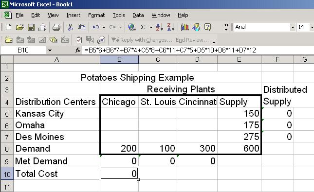
76 Transportation Example A transportation model is formulated for a class of problems with the following characteristics: a product is transported from a number of sources to a number of destinations at the minimum possible cost each source is able to supply a fixed number of units of product each destination has a fixed demand for product

77 Transportation Example Demand and Supply needs

78 Transportation Example Transportation Costs among plants and distribution centers

79

80 Transportation Example Solution

81 A simple Supply Chain 5 production plants (A, B, C, D, E) and 6 retail shops (1, 2,..., 6) Each plant has a predefined capacity, a fixed production costs and a variable production cost per unit of product produced Each store has a minimum supply requirement (customer demand + safety stock) and a sale price For the transportation of product from each plant at each retail store there is a predefined transportation cost Problem: Find the optimum production and distribution quantities at each node Maximize the profit

82 Simple Supply Chain Input Data: Variable Cost Fixed Cost Capacity A 52 75, B 63 35, C 57 50, D 49 41, E 67 22, Demand Price

83 Simple Supply Chain Variables: Y A = 1, if plant A operates, 0 otherwise Y B,..., Y E 0/1 binary variables the other plants A 1 = quantity that is produced in A and it is transported to retail shop 1 Respectively: A 2,..., A 6, B 1,..., E 6 0 continuous variables that correspond to the quantities that produced and transported to the retail shops

84 Simple Supply Chain Max Z = 38 A A A A A E 6 --(75.000Y A Y B Y E ) s.t. A 1 + A A 6 18 Y A B 1 + B B 6 24 Y B E 1 + E E 6 31 Y E A 1 + B E 1 10 A 2 + B E 2 8 Δυναμικότητα Capacity Demand Ζήτηση A 6 + B E 6 11 A 1,..., E 6 0 Y A, Y B,..., Y E = 0/1

85 Simple Supply Chain Decision Variables Retail Stores (Flow Variables) Plants A B C D E Plants Binary variables A 0 B 1 C 0 D 0 E 1 Objective Function Coefficients Capacity Constraints 0 <= 0 24 <= 24 0 <= 0 0 <= 0 31 <= Totals Target Cell Demand Constraints 10 >= 10 8 >= 8 12 >= 12 6 >= 6 7 >= 7 12 >= 11

86 Using Excel Solver Useful tips

87 Using Excel Solver Two steps: Model development decide what the decision variables are, what the objective is, which constraints are required and how everything fits together Optimize systematically choose the values of the decision variables that make the objective as large or small as possible and cause all of the constraints to be satisfied.

88 Using Excel Solver Excel terminology for optimization Decision variables = changing cells Objective = target cell Constraints impose restrictions on the values in the changing cells. A common form for a constraint is nonnegativity Nonnegativity constraints imply that changing cells must contain nonnegative values.

89 Using Excel Solver Real-life problems are almost never exactly linear. However, a linear approximation often yields very useful results. In terms of Solver, if the model is linear the Assume Linear Model box must be checked in the Solver Options dialog box. Check the Assume Linear Model box even if the divisibility property is violated.

90 Using Excel Solver If the Solver returns a message that the condition for Assume Linear Model are not satisfied it can indicate a logical error in your formulation. can also indicate that Solver erroneously thinks the linearity conditions are not satisfied. Try not checking the Assume Linear model box and see if that works. In any case it always helps to have a well-scaled model.

91 Using Excel Solver Infeasibility and Unboundedness It is possible that there are no feasible solutions to a model. There are generally two possible reasons for this: 1. There is a mistake in the model (an input entered incorrectly) or 2. the problem has been so constrained that there are no solutions left. In general, there is no foolproof way to find the problem when a no feasible solution message appears.

92 Using Excel Solver A second type of problem is unboundedness. Unboundedness is that the model can be made as large as possible. If this occurs it is likely that a wrong input has been entered or forgotten some constraints. Infeasibility and unboundedness are quite different. It is possible for a model to have no feasible solution but no realistic model can have an unbounded solution.