International Trade, Monopolistic Competition and Gravity

Transcription

1 International Trade, Monopolistic Competition and Gravity Dennis Novy Spring Term 2015 EC9B3 Topics in Macroeconomics and International Trade

2 We will cover two main topics. (1) Monopolistic Competition and International Trade (2) Gravity We will discuss a number of key papers from the literature. The precise references are provided in the reading list.

3 (1) Monopolistic Competition and International Trade

4 Krugman (1979, 1980) Monopolistic competition is a particular market structure where many key (theoretical) contributions were made in the 1970s. Probably the most famous reference is Dixit and Stiglitz (1977) who developed the CES (constant elasticity of substitution) case. Paul Krugman saw the potential of these developments for the international trade literature. He combined it with increasing returns to scale (scale economies).

5 This leads to intra-industry trade (as opposed to inter-industry trade based on neoclassical models of comparative advantage such as Ricardo and Heckscher- Ohlin). His breakthrough contributions along those lines (including applications to economic geography) eventually won Krugman the Nobel prize in 2008 (as a rare solo recipient).

6 What are the main features of monopolistic competition? Monopolistic competition is a model of an imperfectly competitive industry. It is a special case of oligopoly. It assumes that: Each firm can differentiate its product from the product of competitors (no homogeneous goods). These differentiated products (or varieties ) are good but not perfect substitutes. They may differ slightly in terms of branding, quality or location. Example: different varieties of toothpaste on supermarket shelves. Thus, there is competition but not perfect competition. Each firm ignores the impact of changing its own price on the prices set by its competitors (no strategic interaction): even though each firm faces competition, it behaves as if it were a monopolist and sets the profit-maximising price for its product. But in the long run, the entry of new firms (i.e., new varieties) drives profits down to zero.

7 Monopoly profits rarely go uncontested because they attract market entry of other firms. A firm in a monopolistically competitive industry is expected: to sell more the larger the total sales of the industry and the higher the prices charged by its rivals, to sell less the larger the number of firms in the industry and the higher its own price.

8 A review of monopoly

9 Neoclassical inter-industry trade

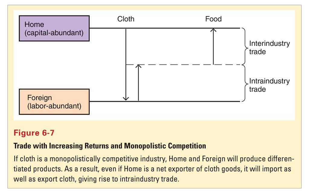
10 Intra-industry trade

11 Intra-industry trade is empirically important

12 Krugman (1980) Utility function is CES U = i c θ i with 0 < θ < 1 and n the number of goods actually produced. For θ 1 we would move towards perfect substitutability. For θ 0 the love of variety effect becomes very strong. in standard notation where σ is the elasticity of sub- θ corresponds to σ 1 σ stitution. Note that 0 < θ < 1 implies σ > 1. (For inelastic demand 0 < σ < 1 we would have negative marginal revenue.)

13 Production function with labour as the only input (one-factor model) l i = α + βx i with α, β > 0. Thus, fixed cost and constant marginal cost with symmetric firms. Scale economies are internal, not external. Market clearing x i = Lc i where L is the labour force (not mobile across countries). Full employment L = n i=1 (α + βx i )

14 Assume free entry/exit such that profits are zero in equilibrium. Firms ignore the effect of their pricing decisions on other firms (no strategic interaction). First-order condition from utility maximization θc θ 1 i = λp i where λ is the Lagrange multiplier (shadow price, i.e., the marginal utility of income). Can be rearranged to obtain demand for a single firm as ( ) xi θ 1. p i = θ λ L

15 Since the effect on λ is ignored by firms, each firm faces a demand curve with elasticity 1 1 θ. To see this solve for x i and then form the elasticity. The profit-maximizing price follows as p i = βw θ where w is the wage. Due to symmetry we have p i = p. Note that βw is the marginal cost, and 1/θ is the markup factor.

16 Profits are π i = px i (α + βx i ) w π = 0 implies again x i = x. x i = αθ β(1 θ) The number of firms follows (also taking full employment into account) as n = L α + βx = L(1 θ) α

17 What about free trade (zero trade costs τ = 0) with another country that has the same preferences and technology? Trade increases the size of the market. But firms will not locate in both countries (otherwise they would incur twice the fixed cost). The model is silent on the precise location chosen by each firm. Thus, the direction of trade is indeterminate. But the volume of trade is not. In practice, this leaves room for history and accident. Symmetry ensures the same wage rate and the same price everywhere.

18 The number of firms/varieties is given by n = L(1 θ) α, n = L (1 θ) α Home consumers spend the fraction n+n n of their income on Foreign goods. The fraction is n n+n in the opposite direction. Value of Home imports from Foreign is Lwn+n n = LwL+L L, which is the same in the opposite direction. Thus, trade is balanced. Due to symmetry p and w are the same across countries and as in the closed economy. Thus, the real wage w/p remains unchanged.

19 But consumer welfare improves due to a variety effect (increased product diversity): n + n > n, n. This is the sole source of gains from trade. x also remains unchanged (no effect on production scale). To get an increase in scale, we need demand to become more elastic as the number of firms goes up. Seems plausible since more finely differentiated products should be more substitutable. See Krugman (1979).

20 What about costly trade (positive trade costs τ > 0)? Introduce iceberg trade costs: the fraction τ of goods melts away in transit, only the fraction 1 τ arrives. The price Home consumers have to pay for Foreign goods follows as p 1 τ where p is the price in Foreign faced by Foreign consumers, and vice versa. Trade costs have no effect on the firms pricing policies, and p/w and p /w are as previously. We still have n and n as above. However, the relative wage is generally no longer w/w = 1. Main result: The larger country will ceteris paribus have the higher wage rate.

21 Intuition: Workers are better off in larger countries because those can better reap the increasing returns. The home market effect : Firms have an incentive to concentrate production (due to increasing production) near the largest market (to minimize trade costs). In a two-industry two-country model, a country will be a net exporter of the product for which it has the larger domestic demand (the home market). Specialization will occur if the two countries have suffi ciently dissimilar tastes (i.e., suffi ciently larger domestic demand). Note that the cause of specialization is demand-driven, not comparative advantage as in neoclassical models.

22 Specialization will be incomplete otherwise (the greater τ and the smaller the fixed cost α).

23 Krugman (1979) Utility function is more general than CES: U = i v (c i ), v > 0, v < 0 First-order condition for utility maximization: or expressed as inverse demand: such that v (c i ) = λp i, p i (c i ) = v (c i ) λ d p i d c i = v (c i ) λ,

24 or d c i d p i = λ v (c i ) Elasticity of demand follows as ε i = d c i d p i p i c i = v (c i ) c i v (c i ) with the assumption ε i c i < 0 ( I make the assumption without apology. ) Thus, the elasticity is variable! It is decreasing in consumption. Intuition: A firm has more market power the larger its market share.

25 The price follows as p i = ε i ε i 1 βw The effects of growth in the labour force L (which is the same as opening up costless trade with another symmetric country): Output of each good x i and the real wage w/p rise (in contrast to CES case), and n rises. Thus, two channels of welfare gains: higher real wages, more variety.

26 Melitz (2003) Melitz extended the basic Krugman model by introducing heterogeneous as opposed to symmetric firms. Consistent with reality: Performance varies dramatically across firms. Some firms are large, some are small. Only a subset of firms exports. Melitz seminal work has inspired much innovative new research (theoretical and empirical) in the international trade literature. Key intuition: Increased competition (through economic integration) hurts the worst-performing firms the hardest as they tend to be the ones that exit.

27 But economic integration also means new sales opportunities in new markets. The best-performing firms take greatest advantage of those opportunities and expand the most. Thus, economic integration leads to a change in the composition of firms in a given industry. Better-performing firms expand while worse-performing firms contract or exit. Overall industry performance thus improves. Empirically, those composition changes lead to substantial improvements in industry productivity. Heterogeneity is introduced by firms having different cost curves (i.e., supplyside heterogeneity).

28 Firms face the same demand curve (i.e., no demand-side heterogeneity/idiosyncratic demand).

29 Performance differences across firms

30 What happens when the economy opens up to international trade? Two effects: As the integrated market supports more firms, the intercept of the demand curve goes down (n goes up). The slope flattens because market size S increases. Demand therefore shifts in for the smaller firms (i.e., the least productive ones) that operate on the top part of the demand curve (where prices are relatively high).

31 Winners and losers from economic integration

32 With positive trade costs τ > 0, we get selection effects: only the strongest firms will export. In the typical U.S. manufacturing industry, an exporting firm is on average more than twice as large as a firm that does not export. Most U.S. firms do not report any exporting activity at all they only sell to U.S. customers. In 2002, only 18% of U.S. manufacturing firms reported any sales abroad. The same pattern is true for other countries including the UK. Even in industries that export much of what they produce, such as chemicals, machinery, electronics, and transportation, fewer than 40 percent of firms export.

33 A major reason why trade costs reduce trade so much is that they drastically reduce the number of firms selling to customers across the border (called the extensive margin of trade). Trade costs also reduce the volume of export sales of firms selling abroad (called the intensive margin).

34 Proportion of U.S. firms reporting export sales by industry, 2002

35 Export decisions with trade costs

36 Utility function is CES U = [ ωɛω q(ω)ρ d ω ] 1/ρ with 0 < ρ < 1 and σ = 1 ρ 1 > 1, and where Ω represents the mass of available goods. We have the aggregate good Q U. Price index follows as P = [ ωɛω p(ω)1 σ d ω ] 1 1 σ Demand for an individual variety follows as [ p(ω) q(ω) = Q P just as in Dixit and Stiglitz (1977). ] σ

37 Production function for an individual firm is l = f + q ϕ where each firm faces f > 0. Firms are indexed by different productivity levels ϕ > 0. The optimal price is set as p(ϕ) = w ρϕ where the wage w = 1 is normalized to one. Profits per firm where r(ϕ) σ is variable profits. π(ϕ) = r(ϕ) l(ϕ) = r(ϕ) σ f

38 Compare the ratio of two firms outputs and revenues: q(ϕ 1 ) q(ϕ 2 ) = ( ) σ ϕ1, ϕ 2 r(ϕ 1 ) r(ϕ 2 ) = ( ) σ 1 ϕ1. ϕ 2 A more productive firm 1 (if ϕ 1 > ϕ 2 ) will be bigger (more output, more revenue), charge a lower price and earn higher profits. Aggregation: Mass M of firms and a productivity distribution µ(ϕ) over (0, ). Then P = [ 0 ] 1 p(ϕ) 1 σ 1 σ Mµ(ϕ) d ϕ Can be written as P = M 1 1 σp ( ϕ)

39 where ϕ = [ 0 ] 1 ϕ σ 1 σ 1 µ(ϕ) d ϕ is a weighted average independent of M. It also represents aggregate productivity since it summarizes all relevant information for aggregate variables: R = P Q = Mr ( ϕ), Q = M 1 ρq ( ϕ), Π = Mπ ( ϕ). Firm entry and exit: A large pool of prospective entrants. All firms are identical ex ante (prior to entry).

40 To enter must pay a sunk cost f e > 0. Then firms draw ϕ from a common distribution g(ϕ) with support (0, ) and cdf G(ϕ). Constant death probability δ of exiting. Only consider steady-state equilibria with constant aggregate variables over time. Each firm s value function is v(ϕ) = max 0, t=0 (1 δ) t { π(ϕ) = max 0, 1 } δ π(ϕ) Note that π(0) = f < 0. In that case exit immediately.

41 Cutoff productivity level ϕ is implied by π(ϕ ) = 0. Thus, a firm with ϕ < ϕ immediately exits and never produces. It follows µ(ϕ) = g(ϕ) 1 G(ϕ ) if ϕ ϕ, 0 otherwise Thus, endogenous µ(ϕ) follows from the exogenous g(ϕ). All incumbent firms (except the cutoff firm) earn positive profits such that average profits π > 0. This expectation is the only reason firms pay f e for entry.

42

43 Equilibrium in closed economy: Firm-level variables such as ϕ and π are independent of country size L. Welfare per worker W = P 1 = M 1 σ 1ρ ϕ is higher in a larger country due only to increased product variety. Similar to Krugman (1980). Equilibrium in open economy: With zero trade costs trade is like increasing L. Introduce trade frictions: fixed costs of entering export markets f ex, can be seen as per-period costs: f x = δf ex. Also per-unit iceberg costs τ > 1

44 (note that this τ notation slightly differs from the one above in the Krugman model). n 1 identical other countries. Revenues are r d (ϕ) = R (P ρϕ) σ 1, r x (ϕ) = τ 1 σ r d (ϕ) Profits are π d (ϕ) = r d(ϕ) σ π x (ϕ) = r x(ϕ) σ f, f x Export cutoff productivity is ϕ x. implied by π x (ϕ x) = 0. Leads to partitioning of firms by export status:

45 If ϕ x = ϕ, then all firms export. If ϕ x > ϕ, then firms with ϕ x > ϕ ϕ produce exclusively for the domestic market. The impact of trade: Let ϕ a and ϕ a denote the cutoff and average in autarky. The exposure to trade increases the cutoff (ϕ > ϕ a). The least productive firms with ϕ > ϕ ϕ a exit (domestic market selection). Only firms with ϕ ϕ x enter export markets (export market selection).

46 Thus, we have a reallocation of market shares towards more effi cient firms and an aggregate productivity gain. The number of firms in a country decreases after trade (M < M a ). But consumer still enjoy greater product variety (M t = (1 + np x ) M > M a ) where p x is the export probability. Overall, we have a type of Darwinian evolution within an industry: the most effi cient firms thrive and grow they export and increase both their market share and profits. Some less effi cient firms still export and increase their market share but incur a profit loss. Some even less effi cient firms remain in the industry but do not export and incur losses of both market share and profit. Finally, the least effi cient firms are driven out of the industry.

47

48 A final comment on the role of CES preferences for the gains from trade: Due to CES there is no increase in product market competition through trade since markups are constant. Instead, selection is driven by the domestic factor market. Firms compete for a common source of labour. Costly entry into export markets affords opportunities only to the more productive firms that can cover the entry cost. This also induces more entry as prospective firms respond to the higher potential returns of a good productivity draw. Increased labour demand bids up the real wage and forces the least productive firms to exit.

49 Chaney (2008) Compared to Melitz (2003), Chaney introduces two main simplifications: Pareto distribution of firm productivity (following Helpman, Melitz and Yeaple 2004), a homogeneous outside good (partial equilibrium). Other key features: multiple asymmetric countries, asymmetric trade costs. Yields extensive and intensive margins of adjustment in response to trade cost changes.

50 Motivation for Pareto productivity distribution: observed size distribution of firms is close (long upper tail). But does not quite match the existence of small exporters. Convenient feature of Pareto (a type of power law probability distribution): truncating a Pareto yields another Pareto.

51 N countries Population L n in country n, production function linear in labour H +1 sectors with a continuum of differentiated goods in each sector apart from sector 0 which provides a homogeneous good. Utility with U = q µ 0 0 H h=1 µ 0 + ( Ω h q h (ω) H h=1 σ h 1 σ h d ω µ h = 1, σ h > 1 ) ( ) σ h σ h 1 µ h

52 Note the isoelastic CES demand, leading to constant markups. No trade costs for good 0 (used as numeraire). Produced under constant returns to scale with one unit of labour producing w n units. Price is set equal to 1. Hence wage is w n. For differentiated goods, both variable trade costs (iceberg: only 1/τ h ij units arrive) as well as fixed trade costs f h ij. Fixed costs of production, so increasing returns.

53 Each firm in sector h draws random unit labour productivity ϕ so that the cost of producing q units becomes c h ij (q) = w iτ h ij ϕ q + f h ij Productivity shocks are Pareto distributed over [1, ) with cdf P ( ϕ h < ϕ) = G h (ϕ) = 1 ϕ γ h and γ h > σ h 1 (ensures that the size distribution of firms has a finite mean). γ h is an inverse measure of heterogeneity: sectors with high γ h are more homogeneous (more output is concentrated among the smallest and least productive firms).

54

55

56 Mass of potential entrants is assumed proportional to w n L n. No free entry assumption. Hence net profits, redistributed to workers in a non-distortionary way.

57 Exports from country i to country j in sector h by a firm with ϕ are with price index P h j = x h ij (ϕ) = ph ij (ϕ)qh ij (ϕ) = µ hy j N k=1 w k L k ϕ h kj σ h σ h 1 w k τ h kj ϕ ph ij (ϕ) P h j 1 σ h 1 σ h d G h (ϕ) 1 1 σ h where ϕ h kj is the productivity cutoff for exporting, coming from the condition π h kj (ϕh kj ) = 0. Let s drop the h subscript for simplicity.

58 In equilibrium, insuffi ciently productive firms cannot generate enough profits from selling abroad to cover the fixed costs of entering the foreign market. Hence, we get extensive margin selection. Equilibrium exports can be solved as x ij (ϕ) = ( )σ 1 Yj γ λ 3 Y ( wi τ ij θ j ) 1 σ ϕ σ 1 if ϕ ϕ ij, 0 otherwise Note that for the intensive margin, the variable trade cost elasticity is σ 1, as standard.

59 Cutoff ϕ ij follows as ϕ ij = λ 4 ( Y Y j )1 γ w i τ ij θ j f 1 σ 1 ij Aggregate exports are Xij h = µ Y i Y j h Y w iτ h ij θ h j h ( ) ( ) γh γ f h σ ij h 1 1 This looks similar to a standard gravity equation (log-linear). The variable trade cost elasticity is the Pareto shape parameter γ h. The fixed trade cost elasticity is a function of both γ h and σ h.

60 Formally, variable trade cost elasticity: so that ζ d ln X ij d ln τ ij = γ ζ σ = 0 Fixed trade cost elasticity: so that ξ d ln X ij d ln f ij = ξ σ < 0 γ σ 1 1 But note that all elasticities are constant, not variable (they only depend on parameters).

61 Melitz and Ottaviano (2008) Compared to Melitz (2003), they introduce variable markups through a linear demand system (nonhomothetic preferences). They also use a Pareto distribution. Preferences where q c 0 U = q c 0 + α iɛω q c i d i 1 2 γ iɛω (q c i )2 d i 1 2 η is consumption of the numeraire good. The parameters α, γ and η are all positive. iɛω q c i d i 2

62 α and η index the substitution pattern between the differentiated varieties and the numeraire: increases in α and decreases in η both shift out demand for differentiated varieties relative to the numeraire. γ indexes the degree of product differentiation between varieties. In the limit when γ = 0 varieties are perfect substitutes when consumers only care about their consumption level over all varieties Q c = iɛω q c i d i Marginal utilities are bounded (positive demand for numeraire is assumed such that q0 c > 0). Inverse demand is given by p i = α γq c i ηqc.

63 (2) Gravity

64 Anderson and van Wincoop (2003) The gravity equation is one of the most used and most empirically successful tools in economics. Relates bilateral trade to size (GDP) and bilateral trade costs. specification: x ij = y iy j t η ij Old-school where trade costs are typically a (loglinear) function of bilateral distance and dummies for (not) crossing an international border (if the data sets includes bilateral trade within a country, say, FL-TX), speaking a common language, having a free trade agreement etc. The trade cost elasticity is η. ln ( t ij ) = ρ ln ( distij ) + ( 1 BORDERij ) + LANGij + F T A ij

65 For instance, McCallum (1995) famously estimates ln(x ij ) = α 1 +α 2 ln(y i )+α 3 ln(y j )+α 4 ln(dist ij )+α 5 ( 1 BORDERij ) +εij using a Canadian-US data set with two types of bilateral trade flows: interprovincial (e.g., Ontario-British Columbia with BORDER ij = 0) as well as province-state (e.g., Ontario-TX with BORDER ij = 1). Anderson and van Wincoop (2003) estimate α 5 = 2.8 for 1993 data, which means that after controlling for distance and size interprovincial trade is exp(2.8) = 16.4 times higher than province-state trade. McCallum (1995) estimates 22 times based on 1988 data. Unbelievably large! Anderson and van Wincoop (2003) show that the previous estimating equation is misspecified and suffers from omitted variable bias. Also, they stress the need

66 to recompute the new general equilibrium if we want to answer the question of by how much will trade go up if we remove the border?

67 The gravity model is an Armington endowment economy (goods are differentiated by place of origin) with CES preferences i 1 σ β σ i c σ 1 σ ij σ σ 1 where σ > 1 and β i > 0 is a distribution parameter. Exporter s supply price is p i. With the iceberg trade cost factor t ij 1 we get p ij = t ij p i. The nominal value of exports is x ij = p ij c ij. The budget constraint is y j = i x ij

68 Nominal import demand by j for goods from i follows as x ij = with price index P j = i ( βi t ij p i P j ) 1 σ y j ( βi t ij p i ) 1 σ 1 1 σ For general equilibrium we need market-clearing y i = j x ij Insert market-clearing into the import demand equation to solve the key gravity

69 equation x ij = y iy j y W ( tij Π i P j ) 1 σ where y W = j y j is world income. The crucial point is that bilateral trade is influenced by the bilateral trade barrier t ij relative to average trade barriers Π i and P j where Π i j ( ) 1 σ tij θ j P j 1 1 σ is the outward multilateral resistance barrier (summed over importers with coun-

70 try weights θ j ) and P j = i ( ) 1 σ tij θ i Π i 1 1 σ is the inward multilateral resistance barrier (summed over exporters with country weights θ i ) with θ j y j y W. Ceteris paribus increasing multilateral resistance increases bilateral trade. Under the assumption of symmetric bilateral trade costs t ij = t ji the system simplifies such that Π i = P i and P j = i ( ) 1 σ tij θ i P i 1 1 σ

71 as well as x ij = y iy j y W ( tij P i P j ) 1 σ Bilateral trade is homogeneous of degree zero in trade costs (including domestic trade costs t ii ). Intuition: The constant vector of real endowments must be distributed. Multilateral resistance P i is homogeneous of degree 1/2 in trade costs. Trade costs cannot be distinguished from preferences (such as home bias).

72 Assume trade cost function ln ( t ij ) = ρ ln ( distij ) + ( 1 BORDERij ) The estimating equation now becomes ln(x ij ) = k + ln(y i ) + ln(y j ) + (1 σ) ρ ln(dist ij ) + (1 σ) ( ) 1 BORDER ij (1 σ) ln(pi ) (1 σ) ln(p j ) + ε ij where k is a constant. Note the two multilateral resistance price indices. Omitted variables in the old-school specification. Unitary income elasticities (nothing unusual with homothetic preferences).

73 Two estimating methods: (1) Nonlinear least squares of gravity equation taking into account the price index equation for each country. P j = i ( ) 1 σ tij θ i P i 1 1 σ

74 An easier (and more common) alternative: (2) Dummy variable estimation to eliminate the multilateral resistance terms (OLS or PPML à la Santos Silva and Tenreyro 2006) For the case of symmetric bilateral trade costs we have country dummies α k k: ln(x ij ) = ln(y i ) + ln(y j ) + (1 σ) ρ ln(dist ij ) + (1 σ) ( ) 1 BORDER ij + α k + ε ij For asymmetric bilateral trade costs we have exporter dummies α i i and importer dummies α j j: k ln(x ij ) = (1 σ) ρ ln(dist ij ) + (1 σ) ( 1 BORDER ij ) + i α i + j Note that the GDP terms are now absorbed by the dummies. α j + ε ij

75

76 Data set: 61 regions (30 US states, 1 rest-of-the-us, 10 Canadian provinces, 20 other countries) For the year 1993 The border estimate of 1.59 = (1 σ) ln(b) = (1 σ) ( 1 BORDER ij ) corresponds to a tariff equivalent b 1 of 48 percent for σ = 5 19 percent for σ = 10 9 percent for σ = 20

77 General equilibrium comparative statics: How would trade flows change if the border were removed? Key methodological innovation: Recompute the general equilibrium and then compare trade with (BB) and without (NB) borders. Multilateral resistances will change. Interprovincial trade increases by 596 percent due to borders. Interstate trade increases only by 25 percent due to borders. Intuition: Multilateral resistances for Canadian provinces increase more strongly so that we see a bigger drop in relative trade resistance t ii P i P for trade within i Canada than within the US.

78 International trade with borders is 56 percent of the hypothetical trade without borders (a reduction of 44 percent). Table 4 below breaks this down into 0.20 (due to bilateral resistance) times 2.72 (due to multilateral resistance) = 0.56.

79

80 Novy (2013) Gravity equations are the workhorse model of international trade for explaining trade flows between countries: x ij = y iy j y W ( tij Π i P j ) 1 σ. Most leading trade models predict a gravity equation: Anderson and van Wincoop (2003): multilateral resistance effects in an endowment economy (1 σ) Eaton and Kortum (2002): Ricardian comparative advantage ( θ)

81 Chaney (2008), Helpman, Melitz and Rubinstein (2008), Melitz and Ottaviano (2008), Behrens, Mion, Murata and Südekum (2009): heterogeneous firms ( γ) Deardorff (1998): Heckscher-Ohlin framework (1 σ) Thus, gravity has a seemingly diverse theoretical foundation. But these models are associated with a constant elasticity of trade with respect to trade costs: d ln ( ) x ij d ln ( ) = constant = σ 1, θ or γ. t ij I call this standard or traditional gravity. Presumably, the predominance of Pareto on the supply side and CES on the demand side lead to isomorphic gravity equations.

82 This paper I introduce an alternative demand system: translog preferences (Christensen, Jorgenson and Lau 1975, Diewert 1976). I derive a micro-founded translog gravity equation in general equilibrium. I compare standard gravity and translog gravity. Why should we care? Allows us to revisit the effect of gravity variables (currency unions, free trade agreements, WTO membership etc.)

83 Translog preferences have some desirable features: - Give a second-order approximation to an arbitrary expenditure function. - Allow for variable substitution effects across varieties (Armington/monopolistic competition): the elasticity of substitution is not constant. - Endogenous markups, and the toughness of competition matters. - Homothetic (unlike quadratic preferences in Melitz and Ottaviano 2008 or Fieler 2010). - In the spirit of Krugman (1979): non-ces.

84 Main results In contrast to standard gravity equations, translog gravity has an endogenous trade cost elasticity depending on how intensely two countries trade with each other. Trade is less sensitive to trade costs if the exporting country has a large market share in the importing country. Intuition: Countries which export a lot to a certain destination have a strong and powerful market position. This position is hardly altered by trade cost changes. Thus, trade costs have a heterogeneous impact across country pairs.

85 Example: If there is a uniform drop in trade costs (for instance, a trade liberalization), then trade will be disproportionately expanded by small exporting countries (see empirical evidence on NAFTA by Kehoe and Ruhl 2009). Translog gravity predicts zero trade flows (zero demand). Cannot be delivered by CES. Empirical evidence: I cast doubt on the standard specification. One-size-fits-all trade cost elasticities are not supported by the data. Instead, translog gravity seems favored.

86

87 Literature context - Numerous translog contributions by Rob Feenstra, for example Feenstra and Kee (2008) on endogenous country productivity, Feenstra and Weinstein (2010) on welfare gains through increasing variety. - Translog production functions (Christensen, Jorgenson and Lau 1971); consumption literature related to AIDS (Deaton and Muellbauer 1980) and PIGLOG (Muellbauer 1975 and 1976): typically closed economy and no role for trade costs. - Arkolakis, Costinot and Rodríguez-Clare (2010): continuous translog with Pareto yields the standard log-linear gravity equation. - Gohin and Femenia (2009): bilateral translog estimation in the food industry but without trade costs. - Volpe Martincus and Estevadeordal (2009) use a translog revenue function but not a gravity equation.

88 The model - International trade in general equilibrium with trade costs. - J countries with j = 1,..., J and J 2. - Endowment economy: each country is endowed with at least one good. The number of goods may vary across countries (Armington assumption). N is total number of goods in the world. - Translog expenditure function (Diewert 1976): ln(e j ) = ln(u j ) + α 0j + where γ km = γ mk. N m=1 α m ln(p mj ) N N m=1 k=1 γ km ln(p mj ) ln(p kj ),

89 - p mj is the price of good m when delivered in country j. - Trade frictions such that p mj = t mj p m where p m is the net f.o.b. price of good m and t mj is the variable trade cost factor with t mj 1. - Assume symmetry across the goods from the same country i in the sense p m = p i and t mj = t ij if good m originates from country i. But bilateral trade costs may be asymmetric such that t ij t ji is possible. - To ensure homogeneity of degree one impose N m=1 α m = 1 and N k=1 γ km = 0.

90 - I also require all goods to enter symmetrically in the γ km coeffi cients (see Feenstra 2003): γ mm = γ N (N 1) m and γ km = γ k m with γ > 0, N consistent with homogeneity of degree one. - The expenditure share s mj of country j for good m can be obtained by differentiating the expenditure function with respect to ln(p mj ): s mj = α m + N k=1 γ km ln(p kj ). - Let x ij denote the value of trade from country i to country j, and y j is the income of country j equal to expenditure E j. Then the import share x ij /y j is the sum of

91 expenditure shares s mj over the range of goods that originate from country i: x ij y j = N i m=n i 1 +1 s mj = N i m=n i 1 +1 α m + N k=1 γ km ln(p kj ). - To close the model I impose market-clearing: y i = J j=1 x ij i.

92 Digression: The elasticity of demand and markups (Feenstra 2003) - Take the symmetric case for the expenditure share on good m (dropping the country index j): s m = 1 N γ N (N 1) ln(p m) + N k=1,k m γ N ln(p k) = 1 N + γ ( ln (p) ln (p m ) ), where ln (p) N k=1 ln(p k )/N. Thus, a 1 percent increase in p m (holding the mean log price fixed) lowers its expenditure share by γ percentage points.

93 - The elasticity of demand is ε m = 1 d ln(s m ) d ln(p m ) γ(n 1) = 1 + > 1. Ns m The restriction γ > 0 ensures that the elasticity exceeds unity. - If N is large (e.g., goods continuum), then ε m simplifies to ε m = 1 + γ/s m. Differentiating with respect to ln(p m ) yields d ln(ε m ) d ln(p m ) = γ d s m s 2 m d ln(p m ) = The elasticity is increasing in price. ( γ s m ) 2 > 0.

94 - The markup of prices over marginal costs can be expressed as p m mc m 1 = If the markup is low, use approximation = Then solve for optimal price ln(p m ): 1 ε m 1 = s mn γ(n 1) 1 γ(n 1) N ( ln (p) ln (pm ) ). N 1 p m mc m 1 ln ln(p m ) 1 2 ln(mc m) N ( pm k=1,k m mc m ). ln(p k ) N γ(N 1). Thus, the optimal price puts approximately half the weight on marginal costs and the other half on competitors prices. If N grows, then the final term decreases that is, prices fall due to an increase in variety.

95 Translog can be seen as a form of price-decreasing competition in the spirit of Zhelobodko, Kokovin, Parenti and Thisse (2012): However, as seen above, such a specification [i.e., translog] generates price-decreasing competition only, and thus the possibility of price-increasing competition in some sectors cannot be tested.

96 The translog gravity equation Solve for general equilibrium to obtain the translog gravity equation x ij = y i y j y W γn i ln ( ) t ij + γni ln ( ) J T j + γni s=1 y s y W ln ( ) tis where n i N i N i 1 denotes the number of products of country i. ln ( T j ) is a weighted average of trade costs over the trading partners of country j akin to inward multilateral resistance in Anderson and van Wincoop (2003), given by T s, ln ( T j ) = 1 N N k=1 ln ( t kj ) = J s=1 n s N ln ( ) t sj. The first and last terms on the right-hand side of the translog gravity equation can

97 be captured by an exporter fixed effect S i : S i y i y W + J s=1 y s y W γn i ln ( ) tis T s. Thus, x ij = γn i ln ( ) t ij + γni ln ( ) T j + Si. y j The dependent variable in translog gravity is the import share x ij /y j in levels, not in logarithms. Can also be written as the import share per good: x ij /y j = γ ln ( ) ( ) t ij + γ ln Tj + Si /n i n i = γ ln ( t ij ) + Ŝj + Ŝi.

98 Comparison to standard gravity Take the Anderson and van Wincoop (2003) gravity equation: x ij = y iy j y W ( tij Π i P j ) 1 σ, where Π i and P j are outward and inward multilateral resistance variables. Take the import share x ij /y j as the dependent variable, take logarithms and capture y i, y j, Π i, P j by exporter and importer fixed effects: ( ) xij ln y j = (σ 1) ln ( t ij ) + S i + S j.

99 The trade cost elasticity defined as: ) η d ln ( x ij /y j d ln ( ). t ij - For CES gravity: η CES = (σ 1). - For translog gravity: η translog = γn i x ij /y j. η translog varies across import shares. Its absolute value decreases in the import share. This is a testable implication.

100 Data Trade flows amongst 28 OECD countries (all except the Czech Republic and Turkey) for the year Taken from the IMF Direction of Trade Statistics, GDP data from the IMF International Financial Statistics. Trade cost function: Follow the standard log-linear specification ln ( t ij ) = ρ ln ( distij ) + δ adjij, where ρ denotes the distance elasticity of trade costs. Great-circle distance between capital cities. adj ij is an adjacency dummy.

101 Number of goods: 1) Try n i = n i. 2) Get data on the extensive margin (number of goods) per country from Hummels and Klenow (2005) as a proxy for n i. For example, 0.91 for US, 0.79 for Germany, 0.72 for Japan, 0.05 for Iceland, 0.03 for Luxembourg. 3) Use simple count data from Comtrade at six-digit level (correlation with Hummels and Klenow measure is 77 percent).

102

103

104 Two testable hypotheses Translog gravity implies that the absolute value of the trade cost elasticity decreases in the import share. I form two hypotheses to test this implication. Hypothesis A is based on estimating the standard gravity equation where I allow the distance coeffi cient to vary across import shares h. For simplicity, I drop the adjacency dummy from the notation. I estimate ln ( ) xij y j = λ h ln ( dist ij ) + S i + S j + S h + ω ij, where the distance coeffi cients λ h are allowed to vary over import shares h with h = 1,..., H. I set H = 5. Hypothesis A states as predicted by the constant elasticity gravity model that the λ h distance coeffi cients do not vary across import share intervals, that is, λ 1 =... =

105 λ H. The alternative is as predicted by the translog gravity model that the λ h distance coeffi cients should vary systematically across import share intervals, that is, λ 1 > λ 2 >... > λ H. How should the intervals be chosen? If based on observed import share values, selection would be based on the dependent variable and thus endogeneity bias (Monte Carlo simulations confirm an upward bias in that λ h would be pushed towards zero since dependent variable and interval classification would be positively correlated with the error term). Solution: Choose intervals based on predicted import shares from a first-stage regression with a common distance coeffi cient.

106

107 Hypothesis B is based on the translog estimating equation: x ij /y j n i = κ h ln ( ) dist ij + Ŝi + Ŝj + Ŝh + υ ij, where I again allow the distance coeffi cients κ h to vary over import shares. Hypothesis B states as predicted by the translog gravity model that the κ h distance coeffi cients do not vary across import share intervals, that is, κ 1 =... = κ H. The alternative is as implied by the standard gravity model that the κ h distance coeffi cients should increase in the import share, that is, κ 1 < κ 2 <... < κ H. Again, choose import share intervals based on predicted values.

108

109 Interpretation: Heterogeneous impact of trade costs Use the translog distance coeffi cient to compute the translog trade cost elasticities: η translog = γn i x ij /y j. The values for n i and x ij /y j are given by the data. The translog parameter γ can be retrieved from the distance coeffi cient in the translog gravity estimation, say, γρ = in column 1 of Table 1, where ρ is the distance elasticity of trade costs from the trade cost function. What about ρ? In column 1 of Table 2 I estimate (σ 1)ρ = 1.239, consistent with Disdier and Head (2008). For σ = 8 this implies ρ = The translog parameter then follows as γ = (Feenstra and Weinstein 2010 estimate γ = 0.19 with four-digit data in a supply and demand system).

110 - The Australian import share of New Zealand output is x ij /y j = 0.072, corresponding to η = 1.3: If trade costs go down by 1 percent, the import share should increase by 1.3 percent. - The US import share of New Zealand output is x ij /y j = 0.038, corresponding to η = 4.0: If trade costs go down by 1 percent, the import share should increase by 4 percent. - The Japanese import share of New Zealand output is x ij /y j = 0.024, corresponding to η = 5.0: If trade costs go down by 1 percent, the import share should increase by 5 percent. - The UK import share of New Zealand output is x ij /y j = 0.009, corresponding to η = 14.4: If trade costs go down by 1 percent, the import share should increase by 14.4 percent.

111 CES would imply an elasticity of 7 (= σ 1) but uniform over all import shares ( one size fits all ). Not borne out by the data.

112

113 Box-Cox transformation - Standard gravity and translog gravity are non-nested models. - Look at Box-Cox transform: ( xij /y j n i ) (θ) = ( xij /y j n i ) θ 1 θ - θ = 1 corresponds to linear (translog) case, θ = 0 corresponds to log-linear (standard) case. - θ is estimated at with a standard error of : both the linear and the log-linear case are rejected.

114 Multiplicative error term and NLS estimation - Estimate x ij = [ γn i ln ( ) dist ij + γni ln ( ) ] T j + Si e ε ij, y j where ε ij is assumed normally distributed (i.e., e ε ij is log-normally distributed). - Signs and significance of coeffi cients the same as before. - R-squareds are substantially higher at Reason: for larger import shares the translog model tends to underpredict. Thus, the specification with an additive error term struggles with large values. - But in case of the multiplicative error term, the relatively fat right tail of the lognormal distribution is better able to capture large import shares.

115

116 General equilibrium effects - The distance elasticities in the tables reflect the direct effect of distance on the import share but not the indirect effect through multilateral resistance. - Can multilateral resistance effects explain the declining pattern of absolute distance coeffi cients? - I decompose the change in the import share: ln ( ) xij y j = (1 σ) ln(t ij ) + ln ( ) yi y W + (σ 1) ln(p i P j ). - How does the decomposition change across import shares? - I simulate a one-percent drop in trade costs ( ln(t ij ) = 0.01).

117 - Multilateral resistance effects are largest for the largest import shares (which tend to be associated with the smallest countries). Thus, they dampen the total effect. - But the regression coeffi cients in the tables do not reflect these multilateral resistance effects. Confirmed with Monte Carlo simulations. - Can multilateral resistance effects explain the declining pattern of absolute distance coeffi cients? No.

118

119 Conclusion: Open research questions - Apply translog estimation to other well-known gravity variables: border effects, tariffs, currency unions, free trade agreements, WTO membership, colonial history etc. - Apply translog gravity to disaggregated data at the industry or product level. OECD three-digit industries: translog gravity looks promising. - Nontradable goods and extensive/intensive margins. - Nest CES and translog in a unified framework, use quadratic mean of order r aggregator function (Diewert 1976): f r (x) N N m=1 k=1 a mk x r/2 1/r m x r/2 k.