Data Analysis and Statistical Methods Statistics 651

Size: px

Start display at page:

Download "Data Analysis and Statistical Methods Statistics 651"

Merry Veronica Bond
6 years ago
Views:

1 Data Analysis and Statistical Methods Statistics Lecture 7 (MWF) Analyzing the sums of binary outcomes Suhasini Subba Rao

2 Introduction Lecture 7 (MWF) The binomial distribution So far we have discussed random variables and the probabilities associated with them. In statistics we often want to fit statistical models/distributions to the data (and the associated probabilities). By fitting a model we can do things like predict or check whether certain variables have an influence on an outcome. Modelling will form a large component of any follow-up course (such as STAT652). Model fitting is not the main focus of this class. We will use it as a motivation for introducing the Binomial and Normal distribution. In this lecture we introduce the binomial distribution. We calculate the 1

3 binomial probabilities in simple situations (by hand) and use software to calculate more complex probabilities. We will also introduce the notion of a hypothesis test, which we will return to in later lectures. 2

4 The binomial distribution This is an important distribution for modelling the distribution of categorical data. We often use it to test certain hypothesis. Eg. Whether more people are cured using a new drug treatment over an old treatment. Whether the proportion of people voting in elections now is different to the proportion in the past etc. It is used when several individuals are surveyed and the reply of each individual is a binary random variable. A binary variable is a categorical variable, where the number of choices is two. For example {Yes or No}, {Candidate A or Candidate B}. 3

5 Typically, these variables are encrypted as {1 or 0}. 1 or 0 are not probabilities, they are just a simple way to encode the reply. We assume that the response of each individual is independent of everyone elses response. 4

6 Example 1 Lecture 7 (MWF) The binomial distribution Jack is a happy-go-lucky type of guy. He is so happy-go-lucky that he claims that he does not bother with revising his exam and simply guesses the answers. We want to see whether there is any truth in his claim. In a multiple choice exam (where there is an option of 5 questions) he has a 20% chance of getting the answer correct. If we try to write this formally we can let correct = 1 wrong = 0. So let X= either 1 or 0 depending on whether he gets it wrong or not.. P (He answer the question correctly)=p (X = 1) = 0.2 P (He answers a question incorrectly)=p (X = 0) =

7 Right or wrong are mutually exclusive events (Jack cannot be both right and wrong). Typically, we are not interested on the precise questions he answered correctly, but the total number of questions in the exam he answered correctly. If Jack selects each answer randomly, his score in his exam can take any value from zero to the highest number of marks in the exam. Let S n denote the score out of n questions he did correctly. Then the set of all possible outcomes that S n can take is S n = {0, 1,..., n}. To each outcome has a certain chance of happening. This is the probability he will score that number of marks in the exam i.e. P (S n = k) (for 0 k n). If he guessed each question, then these probabilities 6

8 follow a Binomial distribution Bin(n, p = 0.2) (where n are the number of questions). We give some examples below. 7

9 Deriving the binomial distribution Deriving the distribution of S 2 = X 1 + X 2 (score when there are two questions in exam) Deriving the distribution of S 4 = X 1 + X 2 + X 3 + X 4 (score when there are four questions). It is clear that S 4 can take any of the values {0, 1, 2, 3, 4}. Suppose Jack does 4 questions what is the probability he will get 1 answer correct? This can be written as P (S 4 = 1). Suppose Jack does 4 questions what is the probability he will get he will get 2 answers correct. That is P (S 4 = 2)? Evaluate P (S 4 = 0), P (S 4 = 3) and P (S 4 = 4). 8

10 Solution Lecture 7 (MWF) The binomial distribution Software plots the distribution (the probability of each possible outcome) and the probabilities. 9

11 The binomial distribution This is a formal definition of the binomial distribution. Let X i be the outcome of the ith trial (this is often called a Bernoulli trial). X i can take the value {0, 1} (eg. wrong or correct/yes or no). To these two outcomes we associate a probability P (X i = 1) = p and P (X i = 0) = 1 p (in the example above P (X = 1) = 0.2 and P (X = 0) = 0.8). Often p = proportion of successes in the population We suppose that each trial is independent, that is X 1,..., X n are independent random variables (for example, the chance Jack gets one 10

12 answer correct is completely independent of the chance of Jack getting another correct). We may observe all the random sample X 1, X 2,..., X n. We are interested in the number of successes out of n, this is given by S n = X X n. Since X i is a random variable, then S n is also a random variable which can take any one of the outcomes {0, 1, 2,..., n}. Each outcome has a certain chance of occuring. This chance is given by the formula P (S n = k) = n! (n k)!k! pk (1 p) n k n! = n (n 1) (n 2)... 1 (0! = 1). 11

13 The above formula looks complicated but it simply extends the arguments we have used previously. n! (n k)!k! are the number of outcomes where S n = k and p k (1 p) n k is the probability of one of these outcomes. You do not have to remember this formula! Notation We often say that S n Bin(n, p). To mean that the distribution of S n is binomial, where the probability of a yes in each trial is p and number of trials n. 12

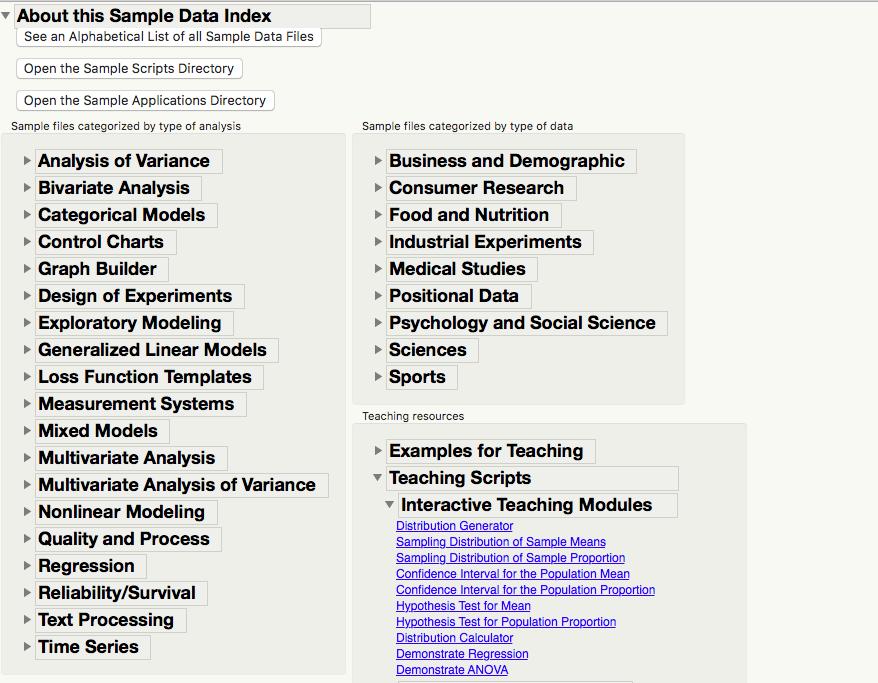
14 JMP: Calculating binomial and other probabilities You can do this using the free non JMP app You can also use JMP. Ensure you have the latest version of JMP Pro 13. Go to (using username and pw given previously). In the folder jmp13 download and run the two files jmpupdater 1310 and Without the latest version, the Distribution Calculator will not work well (or at all). To calculate binomial probabilities in JMP go to Help > Sample Data > Teaching Resources > Teaching Scripts > Interactive Teaching Modules. Select Distribution Calculator (which is highlighted in blue). 13

15 14

16 Example 2 Lecture 7 (MWF) The binomial distribution The formula looks nice, but one can easily use computers to get the probabilities. In this question we will utilize Statcrunch/JMP to answer the question. Jack has taken his final exams. He boasts to his friends that he has been guessing all his answers. He takes two multiple choice exams. In his Biology exam he scores 18 out of 30. In his Chemistry exam he scores 8 out of 30. What do you think about his claims about simply randomly choosing the answer? 15

17 Example 2 as a hypothesis test We formulate this question as a hypothesis test. There are two competing ideas (0) he guessed (A) he had some idea about the material. We are asking, based on his grades, if there is any evidence to prove that he knew the material (can we prove (A)). We state the two competing ideas as two competing hypothesis; the so called null hypothesis, denoted as H 0, is H 0 he guessed. The competing hypothesis is usually called the alternative and denoted as H A (or H 1 ), is that he knew some of the material. In terms of the binomial distribution p = 0.2 corresponds to the case he 16

18 was guessing and p > 0.2 corresponds to the case that he knew some of the material. Using this we rewrite the two competing hypotheses as H 0 : p 0.2 vs H A : p > 0.2. We can only prove H A (prove the alternative hypothesis) by disapproving H 0 (disapprove the null hypothesis). We assess the validity of this claim (the validity of the null) by calculating the chance of obtaining the score he got or even better under the assumption his claim is true. The smaller this probability the less credibile his claim is. It should be stressed that this probability is not the probability of his claim being true. 17

We note that the probability of scoring 18 or more out of the 30

19 Jack s Biology exam We calculate the chance of obtaining 18 or better out of 30, when only guessing. We note that the probability of scoring 18 or more out of the 30 in an exam is P (S p = 0.2) = P (S 30 = 18 p = 0.2) P (S 30 = 30 p = 0.2)

20 This probability implies the chance of him guessing 18 or more is Or in other words, if Jack were to do 10 7 exams (where he just guess all the answers), in about 18 of these exams he would score 18 or more points out of 30. This probability is called a p-value, it is the chance of observing the given data under the scenario that the null hypothesis is true. Rare events, such as this can happen. But a more plausible explanation for the score is that the alternative hypothesis, p > 0.2, is true. A score of 18 or more out of 30 is far more likely if the chance of answering a question correctly is greater than by random (p > 0.2). Conclusion; his score in his Biology exam strongly suggests that he was not randomly guessing and the alternative hypothesis is true. 19

21 To understand what is meant by saying the data suggests he p > 0.2; suppose p = 0.5. The probability p = 0.5 means he is not randomly guessing but is making intelligent guesses based on some knowledge (but we assume independence between questions). The chance of scoring 18 or more out of 30 increases considerably (it is 18%). See the plot below. 20

22 Jack s chemistry exam We test H 0 : p 0.2 vs H A : p > 0.2, based on his scoring 8 out of 30 in his chemistry exam. Using software we calculate P (S 30 8 p = 0.2) = 0.23 The probability of him getting 8 or more by simply guessing is In other words, if he did 100 exams in about 23 of them he would score at least 8 points out of

23 The p-value for this test is 0.23 and it is not small. Therefore it is plausible he guessed. The score of 8 out of 30 is consistent with him guessing, therefore we cannot reject the null hypothesis. We cannot prove the null is true, as it is impossible to know whether he knew the answers to the 8 questions he answered correctly. Conclusion; there is no evidence in the data to reject the null. Even if the p-value were 100% we cannot accept the null. It simply states that the probability of the data being generated if the null were true is very high. However, the probability under a certain alternative could also be high. Thus based on the data we cannot make a decision about our hypothesis. A power analysis (which we do in a later lecture), will help us understand 22

24 the implications of not rejecting the null (and what can be learnt about the alternative). Remember, the p-value does not give the probability of the null being true. Therefore, even with a p-value of 100% we cannot say the null is true! 23

25 Calculation practice Let X i be the probability the ith randomly selected person wins a game. X i = 0 person losses X i = 1 person wins. P (X i = 0) = 0.9 P (X i = 1) = 0.1. Let S 4 = X 1 + X 2 + X 3 + X 4. (i) Calculate the probability two people out of four will win the game (P (S 4 = 2)). (ii) Calculate the probability that two or less people will win the game (P (S 4 2)). 24

26 We construct all the possible different outcomes that can occur which give S 4 = 2. Outcome Per. 1 Per. 2 Per. 3 Per. 4 Probability P(A)= P(B)= P(C)= P(D)= P(E)= P(F)= Remember each outcome is mutually exclusive to all the other outcomes, so P (S 4 ) = P(A or B or C or D or E or F) = P (A) + P (B) + P (C) + P (D) + P (E) + P (F ). 25

27 Since X 1, X 2, X 3, X 4 are all independent events. Then P(A)=P (X 1 = 1, X 2 = 1, X 3 = 0, X 4 = 0) = P (X 1 = 1)P (X 2 = 1)P (X 3 = 0)P (X 4 = 0) = This gives P (S 4 = 2) = Using the same argument we can show that P (S 4 = 1) = and P (S 4 = 0) = Therefore the probability that two or less win the game is the probability noone wins or one wins or two win: P (S 4 2) = P (S 4 = 0) + P (S 4 = 1) + P (S 4 = 2) =

28 Assumptions of a Binomial Experiment The Binomial distribution is extremely useful. To use the binomial distribution the random sample (experiment) must satisfy the following assumptions: (i) Each experiment (known as a Bernoulli trial) results in two outcomes (often refered as a success (yes) and failure (no)). (ii) The probability of a success in each trial is equal to p. (iii) The trials are independent. See page 145 of Ott and Longnecker. 27

29 The binomial distribution: Example 4 The city wants to estimate the proportion of the population which are unemployed. A random sample of 5 people (without replacement) is taken from all the adults in a city. Each person is asked whether they are employed or not. We assume that the proportion of people unemployed is 0.1. Does our sample (experiment) satisfy the assumptions of a binomial distribution? Calculate the probability that out of five randomly selected people, one person is unemployed and the other four are employed. 28

30 Solution Lecture 7 (MWF) The binomial distribution We recall that we observe X 1, X 2, X 3, X 4, X 5, where X i be the answer of the ith person. X 1 = 1 if the person is unemployed and X 1 = 0 if employed. We want to check whether we have a Bernoulli experiment. Each experiment (person interviewed - bernoulli trial) results in a yes or no. So there are two outcomes. In this case the true p is p = Number of people in city who are unemployed, Number of adults in city and we suppose that p = 0.1 (year 200 value). Clearly P (X i = 1) = 0.1 and P (X i = 0) = 0.9. Hence the probability of each draw is the same. 29

31 The independence assumption is a little bit tricky. P (X 2 = 1 X 1 ) will not be exactly P (X 2 = 1) = p. The reason is that we have to remove observation X 1 from the population. So P (X 2 = 1 X 1 = 1) = Number of people in city who are unemployed 1, Number of adults in city 1 Similarly P (X 2 = 1 X 1 = 0) = Number of people in city who are unemployed, Number of adults in city 1 Comparing P (X 2 = 1 X 1 = 1) with P (X 2 = 1) we see that they are not exactly the same. Recall for independence they need that P (X 2 = 1 X 1 = 1) = P (X 2 = 1). However, if the population is large, P (X 2 = 1 X 1 = 1) and P (X 2 = 1) are very close. In which case the 30

32 independence assumption is close to holding. See Ott and Longnecker, Example 4.6 (page 145) for more details. Example Consider a population of 1000 individuals. The random variable here is whether a randomly selected person is employed or not. Suppose that 250 people in the town are employed. Let X 1 be the employment status of the first person drawn and X 2 be employment status of second person drawn (without replacement). Then we see that and P (X 1 = employed) = , P (X 2 = employed) = P (X 2 = employed X 1 = employed) = , We see that P (X 2 = employed) P (X 2 = employed X 1 = employed), 31

33 hence X 1 and X 2 are not independent. But because 250/100 and 249/999 are very close, they are close to independent. Do not worry if you do not catch this argument. The main thing is if the sample size is small as compared with the population size then we have something close to independent samples and a Binomial experiment. Now we want to calculate the probability that one person out of the 5 is interviewed is unemployed: This means that S 5 = X X 5 = 1. All the possible outcomes which gives S 5 = 1 are: 32

34 X 1 X 2 X 3 X 4 X 5 S Under the assumption that P (X i = 1) = 0.1 the probability of one of these outcomes is (0.1) (0.9) 4 Since there are 5 different outcomes which give S 5 = 1 we have P (S 5 = 1) = 5 (0.1) (0.9) 4 =

35 The binomial: mean and variance Recall that the number of successes out of n, denoted by S n is a random variable taking values in {0, 1,..., n} (eg. S 4 is the number of successes out of 4 and has the outcomes {0, 1, 2, 3, 4}). S n has all the properties of a random variable, we can associate a probability to each outcome (the binomial distribution) and it has a probability plot. Since it has a probability plot, it must have a center and a spread, therefore it has a mean and a variance. The mean of a binomial is n p. This is very clear, for example if the chance of my getting a question correct is 80% and I answer 30 questions, on average I will get = 24 question correct. The standard deviation of a binomial is n p (1 p). 34

Data Analysis and Statistical Methods Statistics 651

Review of previous lecture: Why confidence intervals? Data Analysis and Statistical Methods Statistics 651 http://www.stat.tamu.edu/~suhasini/teaching.html Suhasini Subba Rao Suppose you want to know the