Forecast Combination

Transcription

1 Forecast Combination In the press, you will hear about Blue Chip Average Forecast and Consensus Forecast These are the averages of the forecasts of distinct professional forecasters. Is there merit to averaging (combining) different forecasts? Or is it better to focus on selecting the best forecast?

2 GDP Forecast Let s consider forecasting GDP growth for 010Q1 (first estimate to be released April 30) GDP growth for the four quarters of Q1 009Q 009Q3 009Q4 6.4% 0.7%.% 5.6%

3 Models In p.s. #10, you considered models for GDP AR(3) plus 3 lags of dt3 AR(3) plus 3 lags of dt1 AR(3) plus 3 lags of spread1 AR(3) plus 3 lags of spread10 AR(3) plus 3 lags of junk The model with junk spread had the lowest AIC Let s reconsider the number of lags

4 AIC for different lag structures junk yield lags AR(1) AR() * 554 AR(3) The model with AR lags and lags of junk has the lowest AIC But the models with 1 and 3 AR lags have nearly the same AIC And the models with 3 lags of junk are quite close too

5 Forecasts junk yield lags AR(1) AR() * 4.3 AR(3) The point forecasts are quite different The model selected by AIC is much higher than the AR model The model with 3 lags of junk have quite different forecasts

6 Average Forecast The average of the 1 forecasts is ˆ y average = 1 = 4.4 This is similar to a consensus or Blue Chip forecast. You could imagine these 1 forecasts as coming from different forecasters. Is it useful to combine the forecasts?

7 Pseudo Out of Sample Experiment Split the sample Estimation period: 1954Q 1994Q4 (30 years) Evaluation period: 1995Q1 009Q4 (15 years) Estimate the 1 models using 1954Q 1994Q4 Fix the parameter estimates Use these models to forecast 1995Q1 009Q4 Also, take the average forecast for each period Create out of sample errors for the 1 models And the out of sample error for the average forecast Compare the performance of the methods by RMSE A simplified version of predictive least square (PLS)

8 Out of Sample RMSE RMSE junk yield lags AR(1) AR() *.3 AR(3) RMSE Average forecast.18 The comparisons based on out ofsample RMSE are similar to AIC on full sample The lowest RMSE is.3, achieved by the model with lags of each But the RMSE of the average forecasts (the average across all 1 forecasts) is.18 We achieve a much lower RMSE by this simple averaging! Why? Why is it useful to combine forecasts? Can we do better than a simple equal weighted average?

9 Theory of Forecast Combination Suppose you have forecasts f 1 and f for y Suppose they are unbiased with variances var(f 1 ) and var(f ) and suppose they are uncorrelated. Then if you take a weighted average f = wf w) ( f The variance of the average is var( f ) = w var ( ) f + (1 w) var( f ) 1

10 Equal weights If w=1/ then ( f ) var( ) 1 + f var var( f ) = 4

11 Optimal Weights Minimizing with respect to w, the optimal weight The weight on forecast 1 is inversely proportional to its variance 1 ) (1 ) var( σ w σ w f + = = + = σ σ σ σ σ σ w

12 Multiple Forecasts In general, if you have forecasts f 1,, f M a forecast combination is f = w f + w f + L+ 1 1 w M f M Where the weights are non negative and w 1 + w + L+ wm = 1

13 Optimal weights When the forecasts are uncorrelated, the optimal weights are w m = σ 1 σ m + σ + L+ σ M The weight on the m th forecast is inversely proportional to its variance If they have the same variance, then the weights are all equal

14 Bates Granger Combination Bates and Granger (1969) An early influential paper Suggested using empirical weights based on out ofsample forecast variances w m = ˆ σ 1 ˆ σ m + ˆ σ + L+ ˆ σ Even though this was derived under the assumption of uncorrelated forecasts, this method can work well in practice. M

15 Bates Granger Implementation Take a series of (pseudo) out of sample forecasts and forecast errors Compute forecast variance (square of RMSE) Invert. Normalize by sum across all models

16 Example RMSE junk yield lags AR(1) AR() AR(3) Take the first model with RMSE=.46 Square and invert to find 0.16 Sum across all 1 models is.14 Divide 0.16/.14=0.08 This is the weight for this model/forecast Because the RMSE is similar across models, the weights are very similar, all 0.08 or 0.09 Bates Granger weights essentially are the same as equal weights

17 Granger Ramanathan Combination Granger and Ramanathan (1984) Introduced a regression method to combine forecasts Similar to a Mincer Zarnowitz regression Regress the actual value on the forecasts Two forecasts: y + t = β 1 f1 t + β ft e t

18 Multiple Forecasts y = β f + β f + L+ β f + t 1 1t t M Mt e t Should use a constrained regression Omit intercept Enforce non negative coefficients Constrain coefficients to sum to one

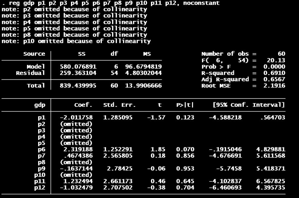
19 STATA implementation reg option noconstant removes the intercept Constrained regression command cnsreg enforces linear constraints defined by constraint For example, if you regress gdp on (p 1,p,p 3,p 4 ).constraint 1 p1+p+p3+p4=1.cnsreg gdp p1 p p3 p4, constraints(1) noconstant

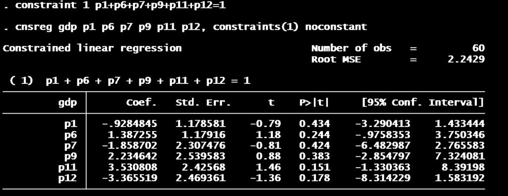
20 Non negativity In STATA it is difficult to enforce the non negative condition on the weights You can do this manually Estimate the regression Eliminate a forecast with the most negative weight Restimate Keep eliminating forecasts until only positive weights are found. Another problem If the forecasts are highly correlated, STATA may exclude redundant forecasts That is okay, they were not helping anyway.

21 Example

22 Example

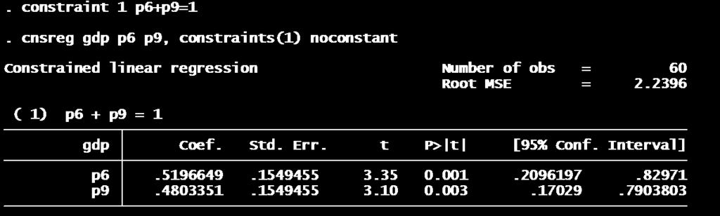
23 Granger Ramanathan Weights and Forecast We found the following estimated weights Model 6: 0.5 Model 9: 0.48 Combination Forecast 0.5* *5.3=4.7%

24 Bayesian Model Averaging In our discussion of model selection, we pointed out that Bayes theorem says that when there are a set of models, one of which is true, then the probability that a model is true given the data is P BIC ( M D) exp 1 These can be used for forecast weights This is a simplified form of Bayesian model averaging (BMA) which is very popular

25 BMA formula We can write the weights as follows Let BIC* be the smallest BIC The BIC of the best fitting model Let ΔBIC=BIC BIC* be the BIC difference = = Δ = M m m m m m m w w w BIC w 1 * * * exp

26 Implementation Compute BIC for each model Find best fitting BIC* Compute difference ΔBIC and exp( ΔBIC/) Sum up all values and re normalize

27 BIC junk yield lags AR(1) * 571 AR() AR(3) ΔBIC/ junk yield lags AR(1) AR() AR(3) weight junk yield lags AR(1) AR() AR(3) BMA puts the most weight on the model with the smallest BIC It puts very little weight on a model which has a BIC value quite different from the minimum In some cases, several models receive similar weight In this example, most weight (75%) goes on the model with the AR(1) plus lags of the junk spread 15% also on AR() plus lags

28 BMA Weights and Forecast BMA Forecast 0.75* *5.1+.0* *4.7+.0*4.3 =5.1%

29 Weighted AIC (WAIC) Some authors have suggested replacing BIC with AIC in the weight formula w m AIC exp There is not a strong theoretical foundation for this suggestion But, it is simple and works quite well in practice.

30 WAIC formula Let AIC* be the smallest AIC The AIC of the best fitting model ΔAIC=AIC AIC* is the AIC difference = = Δ = M m m m m m m w w w AIC w 1 * * * exp

31 AIC junk yield lags AR(1) * 554 AR() AR(3) ΔAIC/ junk yield lags AR(1) AR() AR(3) weight junk yield Lags AR(1) AR() AR(3) WAIC splits weight more than BMA It puts 4% on each of the three models with the best nearequivalent AIC Puts positive weight on 6 models Puts zero weight on 6 models

32 WAIC Forecast WAIC Forecast.4*5.+.4*5.1+.4* * * *4.4 =4.95%

33 Advantages of Combination Methods When the selection criterion (AIC, BIC) are very close for competing models, it is troubling to select one over the other based on a small different In this setting WAIC and BMA will give the two models near equal weight If the selection criterion are different, simple averaging gives all models the same weight, which seems naïve. In this setting WAIC and BMA will give the models different weight And will give zero weight if the different is sufficiently large If the difference in the criterion is above 10.

34 GDP Combination Forecasts AIC Selection: 5.1% BIC Selection: 5.% Simple Average: 4.4% Bates Granger combination: 4.4% Granger Ramanathan combination: 4.7% BMA: 5.1% WAIC: 4.95%

35 Example: Unemployment Rate Estimated on AIC AIC weights BIC BIC weights AR(4) AR(5) *.74 AR(6) AR(7) AR(8) AR(9) AR(10) AR(11) AR(1) AR(13) 1808* AR(14) AR(15) AR(16) AR(17) AR(18) AR(19) AR(0)

36 Out of Sample RMSE Method RMSE AIC.145 BIC.145 BMA.145 WAIC.145 Best Model (AR(1)).143

37 Which should you use? Current research suggests that combination methods achieve lower MSFE than selection BMA achieves lower MSFE than BIC WAIC achieves lower MSFE than AIC Naïve combination (simple averaging) works quite well But the other methods can do better WAIC works well in practice Bates Granger also works well in many settings

38 Forecast Intervals How do you construct intervals for a combination forecast? Do not combine forecast intervals Given the weights, you can construct the sequence of sample forecasts and forecast errors Use these errors as you have before to construct the forecast interval Compute the RMSE of the combination forecast error