MEAN-VARIANCE OPTIMIZATION AND PORTFOLIO CONSTRUCTION: A SHORT TERM TRADING STRATEGY

Transcription

1 MEAN-VARIANCE OPTIMIZATION AND PORTFOLIO CONSTRUCTION: A SHORT TERM TRADING STRATEGY by Michael Leggatt BBA, Simon Fraser University, 2002 and Pavel Havlena BA (Economics), Simon Fraser University, 2001 PROJECT SUBMITTED IN PARTIAL FULFILLMENT OF THE REQUIREMENTS FOR THE DEGREE OF MASTER OF BUSINESS ADMINISTRATION In the Faculty of Business Administration Global Asset and Wealth Management Program Michael Leggatt and Pavel Havlena, 2008 SIMON FRASER UNIVERSITY Fall 2008 All rights reserved. This work may not be reproduced in whole or in part, by photocopy or other means, without permission of the author.

2 APPROVAL Name: Degree: Title of Project: Michael Leggatt and Pavel Havlena Master of Business Administration Mean-Variance Optimization and Portfolio Construction: A Short Term Trading Strategy Supervisory Committee: Dr. Robert Grauer Senior Supervisor Endowed University Professor Dr. Evan Gatev Second Reader Assistant Professor Date Approved: ii

3 ABSTRACT Mean-variance optimization, in theory a very powerful and intuitive tool, has failed to provide meaningful solutions in practical settings, and indeed, in theoretical settings in much past research. Whereas inaccurate statistical estimates for inputs provide even more erroneous outputs, the modeling errors determine outputs that are nothing short of extreme. In this study, we employ two different models based on the mean-variance framework, with one portfolio seeking the highest return given a risk target while the other portfolio seeks the lowest risk given a desired level of return. In unconstrained form, our results confirm to be acutely departed from past experience in this subject matter and contrary to the known literature on modeling errors, our portfolios remain solvent. In constrained form, our portfolios outperform the benchmark and market portfolios while maintaining at least some diversification; in unconstrained form, our portfolios provide surprisingly high absolute and risk adjusted returns with betas less than the benchmark and market portfolios. iii

4 ACKNOWLEDGEMENTS We would like to thank Dr. Robert Grauer for his support and guidance in this research project. Without his relentless commitment to excellence this paper would not have been possible. We would also like to acknowledge the contribution of the entire faculty of the Global Asset and Wealth Management MBA program for providing a truly world class experience and an extraordinary learning environment. iv

5 TABLE OF CONTENTS Approval... ii Abstract...iii Acknowledgements... iv Table of Contents... v List of Figures and Tables... vi 1 INTRODUCTION HYPOTHESIS METHOD Maximize Return Given a Risk Target Minimize Risk Given a Return Target Inputs to Mean-Variance Optimization Rebalancing Frequency Constrained Scenarios Tests Performance Metrics Sharpe Ratio Treynor Ratio Jensen s Alpha RESULTS Maximize Return Given a Risk Target July 1938 to June July 1938 to June 1973 and July 1973 to June Minimize Risk Given a Return Target July 1938 to June July 1938 to June 1973 and July 1973 to June LIMITATIONS SUMMARY APPENDIX A - Histograms APPENDIX B Beta REFERENCE LIST v

6 LIST OF FIGURES AND TABLES Figure 1: A Visual Depiction of Models Table 1: Optimization with Risk Budget Results: to Table 2: Optimization with Risk Budget Results: to Table 3: Optimization with Risk Budget Results: to Table 4: Optimization with Return Target Results: to Table 5: Optimization with Return Target Results: to Table 6: Optimization with Return Target Results: to vi

7 1 INTRODUCTION Selecting the correct mix of assets for an investment portfolio requires more than just finding the most attractive securities. Although all investors demand the highest returns possible from their investment, high returns are generally associated with high risk. Finding the right balance between a portfolio s return and its risk is the central tenet of mean-variance optimization. Mean-variance optimization looks for the mean-variance efficient solution to these following problems: to maximize the expected return for a specified level of risk, to minimize the risk for a specified return, and to maximize the return and minimize the risk given a specified risk parameter. The implication is that investors are willing to trade off return and risk and the amount of return they are willing to give up for a given reduction in risk depends on their risk tolerances or aversions. Following convention 1, the mean-variance model is according to equation 1: Max: (1) s.t. Where µ p is one plus the rate of return, σ² p is the portfolio s variance, and τ is a quadratic programming parameter representing a risk-tolerance measure. 1 Grauer, Robert R Extreme Mean-Variance Solutions: Estimation Error versus Modeling Error. p.6 7

8 Since its introduction by Markowitz (1952) mean-variance optimization has become one of the foundational procedures in portfolio construction. Markowitz showed that for a specified level of risk we can select assets that maximize the portfolio s expected return. He called the mean-variance optimal portfolios efficient and suggested they line up along a frontier in risk-return space. According to his model, rational investors should be investing only in portfolios along the efficient frontier. Even though Markowitz s model provided a framework for the CAPM and many other important studies in the academic community, it was never fully adopted by practitioners. Michaud (1989) claims many practitioners ignore the results or even disregard the practice altogether. He suggests mean-variance optimization tends to maximize the input errors and without appropriate constraints the results are often meaningless. The model also significantly over weights (under weights) securities with large (small) estimated returns, negative (positive) correlation, and small (large) variances. Best and Grauer (1991) confirm the model s sensitivity to estimation errors. With only the budget constraint, small changes in asset means can have a profound influence on the portfolio s weights, mean, and variance. They also show that imposing non-negativity constraints produce extreme portfolio weights while its expected return and standard deviation remain (almost) the same. Using a general form of parametric quadratic programming for sensitivity analysis, Best and Grauer (1991) further show that imposing or relaxing constraints in response to changes in the means changes the portfolio s weights in economically counterintuitive ways. Black and Litterman (1992) suggest that one way to overcome the model s shortcomings is to calibrate its inputs according to investor s specific views about global 8

9 markets. Using this approach apparently produces more balanced and better behaved portfolio that more accurately reflect the investor s preferences. Taking a different approach, Konno and Yamazaki (1991) believe that a large number of assets make it challenging to properly estimate the covariance matrix. Using historical data for the covariance matrix may not be a good approximation of the real correlation structure. Their view is supported by Laloux, Cizeau, Bouchaud, and Potters (1999) who claim that when the correlation matrix is based on historical numbers, the lowest risk portfolios are plagued with noise. It is obvious that estimation errors contribute to the reluctance of investment professionals to adopt mean-variance optimization for portfolio construction. However, a study by Grauer (2001, 2008) provides empirical evidence that modeling errors play a more fundamental role in determining the unrealistic solutions. His results show that using mean-variance optimization without proper constraints, without means based on predictive variables, and without a specific risk tolerance will produce very extreme solutions. There have been numerous recent attempts to make mean-variance optimization practical. Bai, Liu, and Wong (2006), for example, develop new estimators for returns and weights, so-called bootstrap corrected return and bootstrap corrected allocation, using large dimensional matrix theory and the parametric bootstrap method. Their simulation suggests vastly improved accuracy of the estimation process and ease of implementation. Another alternative to the classic mean-variance model is full-scale optimization. Contrary to mean-variance theory, the full-scale model assumes that assets are not normally distributed and investor s preferences cannot be captured by the quadratic 9

10 utility function. Relying on sophisticated search algorithms to identify the optimal portfolio given any set of return distribution and any description of investor preferences, the full-scale optimization calculates the weights that yield the highest possible utility. However, the full-scale procedure suffers from estimation error just like the original mean-variance model. Adler and Kritzman (2006) address this issue by bootstrapping returns from out of sample periods to generate alternative histories. They claim better insample results than the mean-variance model for their study of hedge funds but admit that their model may not outperform the classic mean-variance procedure on other samples or if returns are more normally distributed. Mean-variance theory formalized the risk-reward intuition and provided the necessary framework for other advances in the understanding of institutional investment management and passive investing techniques. Our study both complements the theoretical work on mean-variance optimization and offers alternative methods for investment portfolio selection. We present an approach where investors can optimize their expected portfolio returns given the optimal risk levels obtained from historical returns of the benchmark portfolio. Alternatively, investors can select their assets based on the benchmark returns but with a lower level of risk. To best of our knowledge, our methods have not yet been tested in literature. We can only compare our work to the study by Grauer (2008), where he compares policies and performances of the global minimum-variance portfolio, tangency portfolios, and six mean-variance portfolios and finds that permitting short sales generates rather bizarre outcomes. He shows that in some cases the tangency portfolio s weights are plus and minus thousands of times wealth and many of tangency portfolios are ex ante inefficient. 10

11 Ex post, many of the tangency portfolios, along with most of the mean-variance portfolios, become insolvent. Grauer argues that existing literature focuses mainly on performance metrics and tends to attribute extreme values for expected returns, weights, and standard deviations to estimation error. While he agrees that estimation error is partly responsible for the odd results he suggests that we should focus more on the modeling error of utilizing the mean-variance model with only a budget constraint. Without the short-sale constraint, risk tolerance, and without basing the means on predictive variables the investors may miss out on profitable opportunities. Our models show that relying on historical data, subject to the budget constraint and risk tolerance variable even without the short-sale or predictive means restrictions, the mean-variance model can produce very profitable outcomes This paper proceeds as follows: in the next section the models are formalized and subsequently the methods for implementing them are described in detail. As trading strategies, the models are further reduced to variations in which an investor is limited to the frequency in which he or she can review and rebalance the implemented portfolio. Constraints are also placed on the models to mimic different constraints an investor may face in practice. To test for economic significance risk based performance measures are discussed and then applied to the outcomes of the strategies. Lastly, limitations to the models are presented. 11

12 2 HYPOTHESIS The goal of our empirical work is to create and test two trading strategies based on mean-variance optimization theory. The strategies are based on the tenet that investors will categorically choose one of two portfolios in relation to a given portfolio in every instance: the first would be the portfolio that has the highest expected return for the same level of risk as the given portfolio, and the second would be the portfolio that has a the smallest level of risk for the same level of return as the given portfolio. In simple terms, an investor will maximize return given a risk target, or will minimize risk given a return target. The expectation is that with both these strategies the investor will be able to achieve higher risk adjusted returns over the long run than the investor who accepts the given, or benchmark, portfolio. We test this hypothesis by modeling the trading strategies against a given portfolio and comparing the risk adjusted performance of the implemented portfolios against the given portfolio and the market portfolio. 12

13 3 METHOD The given portfolio (benchmark) is an equal weighted index rebalanced monthly. The benchmark includes 25 assets: each of these assets is an equal weighted basket of stocks with similar size and distress characteristics. The assets and monthly return data are sourced from the 5x5 Fama French factors available on Ken French s data library on his website 2. The data set has been truncated to July 1931 as data for several of the assets is missing prior to that point. Each of the 25 assets represents a basket of equally weighted stocks; the assets have been assigned equal weights in the benchmark portfolio. According to our hypothesis, an investor who has the choice of holding the given portfolio or an alternate combination of the assets within the given portfolio will choose to hold one of two alternate combinations of the assets: the investor will either combine the assets such that the expected return of the implemented portfolio is the highest possible given the level of risk carried by the given portfolio (maximize return given a risk target) or minimize the risk of the implemented portfolio for the level of return achieved by the given portfolio (minimize risk given a return target). In doing so, the investor should achieve better risk adjusted performance than the given portfolio. 3.1 Maximize Return Given a Risk Target An investor will choose to maximize return given a predetermined risk target, all else equal. Equivalently, if two portfolios have equal risk, but one has a higher expected 2 (accessed September 2, 2008) 13

14 return, the investor will choose the portfolio with the higher expected return. To model this behavior we look to our benchmark equal weight portfolio and calculate the standard deviation and average return of that portfolio over the past 84 months (the first history is July 1931 to June 1938). If an investor could construct a portfolio from the assets within the benchmark to obtain the same level of standard deviation that was realized but with a higher expected return moving forward then that would be the portfolio our investor would choose to hold. The model can be expressed according to the following equation: Max: (2) s.t. and In equation 2 the investor is maximizing the expected return of the portfolio by altering the asset weights within the portfolio subject to two constraints: 1) the variance of the constructed portfolio must equal σ 2 p * which is the variance of the benchmark portfolio; and 2) the sum of the weights within the portfolio must equal Minimize Risk Given a Return Target An investor will choose to minimize risk for a predetermined return target, all else equal. Equivalently, if two portfolios have equal return, but one has a lower level of risk, the investor will choose the portfolio with the lower level of risk. To model this behavior we look to our benchmark once again, and calculate the standard deviation and average return of that portfolio over the past 84 months (the first history is again July 1931 to June 1938). If an investor could construct a portfolio from the assets within the 14

15 benchmark to obtain the same level of average return achieved over that period (the investor set this as an expected return target) but with a lower standard deviation by historical estimates then that would be the portfolio our investor would choose to hold. The model can be expressed according to the following equation: Min: (3) s.t. and In equation 3 the investor is minimizing the standard deviation of the portfolio by altering the asset weights within the portfolio subject to two constraints: 1) the expected return of the constructed portfolio must equal r * p which is the average return of the benchmark portfolio over the past 84 months; and 2) the sum of the weights within the portfolio must equal 1. In both models while the investor is constructing the optimal portfolio according to either equation 2 or equation 3 above, the investor can not implement this portfolio until the past 84 months has been observed. As such, we calculate the optimal portfolio weights based on the observed data from July 1931 to June 1938 (month 1 to month 84), and implement our portfolio during the subsequent month (July 1938 month 85). The returns for the optimal portfolios under each model are captured, and the exercise is repeated with a second 84 month history of month 2 to month 85 returns are captured for month 86 (August 1938). This exercise is repeated 840 times with data collected from July 1938 to June In this way, we collect monthly optimal portfolio weights 15

16 based on the benchmark portfolio over 70 years and have portfolio returns for the same frequency and duration. 3.3 Inputs to Mean-Variance Optimization When observing the data over the previous 84 months, the investor is striving to determine the expected asset returns, variances, and covariances as these form the inputs to the portfolio optimization exercise the investor undertakes when fulfilling either of the models presented. For each asset the expected return used in the model is the average return for that asset over the past 84 months. The use of such a return assumes that the return figure is the correct long run expected rate of return for that asset. 84 months provides a reasonable length of time for a return figure to revert to the mean though a casual observation of the average returns shows that in some instances the asset return is negative over the 84 month period. Clearly the expected return for the assets should all be positive or investors would not be persuaded to hold that asset. We do not calibrate the means as Black and Litterman would recommend as it s asset mispricing that allows our investor to construct portfolios superior to the given portfolio. In the same way that the expected return is calculated as the mean return for each asset over the past 84 months, the variance-covariance matrix is calculated based on the asset returns over the past 84 months. The assumption is that the variance-covariance is stable over this length of time. However, as with negative means in the data set, a casual observation of the data shows that certain assets exhibit exceptionally desirable risk/return trade-offs: some assets have very minimal variations in return coupled with 16

17 good returns; other assets have very large variations in return coupled with poor returns. The data is not subjected to any corrections or adjustments. The desired risk target in the risk targeting model is the standard deviation of the benchmark over the past 84 months. The investor will choose to maximize the return of her portfolio, subject to the risk level of the benchmark, for the subsequent period. The desired return target in the return targeting model is the actual average return of the benchmark over the past 84 months. The investor will choose to minimize the risk of the portfolio while achieving a level of return consistent with the average return achieved by the given benchmark portfolio over that period. 3.4 Rebalancing Frequency To this point we ve assumed that an investor has a monthly decision to make with respect to the optimal portfolio weights under either model. However, in practice an investor would certainly be remiss to rebalance monthly as the transaction expenses would significantly erode returns. To add robustness to our models, our investor can choose to rebalance monthly, quarterly, or annually, but can not combine these options. The investor who rebalances monthly will optimize for the subsequent month, as above, and will then do the optimization again each month moving forward to obtain new asset weights within the portfolio. For example, having optimized and held the portfolio through July 1938, the investor will then calculate the average asset returns and the variance-covariance matrix from August 1931 to July 1938, and will set as the risk target the standard deviation of the benchmark over the same period. The optimal portfolio weights calculated using these inputs will then be used as the investor s portfolio weights 17

18 for the subsequent one month holding period (August 1938). The return that the investor achieves in August 1938 is the investor s next one month return. In rolling this exercise forward, the investor constructs an optimal portfolio based on the previous 84 months data, holds that portfolio for one month, and then re-evaluates based on the new previous 84 months data. We run this exercise over the data set and capture the monthly returns from July 1938 to June 2008 for both models. The investor who rebalances quarterly will optimize for the subsequent month, as has been described above in detail, but will then hold that position for 3 months prior to re-evaluating the portfolio holdings. At the end of the three month holding period, the investor will then look to the subsequent 84 month period to determine the inputs to the optimization to determine the holdings for the next three month period. The returns are the three month holding period rate of return for each three month period. We run this exercise over the data set and capture the returns from July 1938 to June 2008 for both models. The investor who rebalances annually will do just as above, but will hold the optimal portfolio position for 12 months prior to re-evaluating the portfolio holdings. At the end of the 12 month holding period, the investor will then look to the subsequent 84 month period to determine the inputs to the optimization to determine the holdings for the next 12 month period. We run this exercise over the data set and capture the annual returns from July 1938 to June 2008 for both models. For the purpose of analysis, the monthly, quarterly, and annual returns that are arrived at using the decision models are compared to the same frequency of realized returns for the benchmark over the same periods. Of note, the benchmark standard 18

19 deviations and returns are invariant to changes in rebalancing frequency. There are two reasons for this: first, the investor has no influence over how the benchmark index is constructed or rebalanced, so trying to adjust it for comparison purposes would be meaningless in real application; second, the monthly equal weight returns in each of the 25 assets is the monthly return for a basket of stocks without knowing the composition of those baskets and the monthly returns of each stock, it s impossible to calculate the true quarterly or annual rebalancing standard deviations and returns. A note on rebalancing frequency: mean variance optimization is typically only useful in a single period setting (the CAPM has shown to be inefficient beyond a single period). Since we are rebalancing monthly, quarterly, and annually, we expect above average returns for a given level of risk to persist, at least in the short term, and vice versa. Assets that have demonstrated above average returns for a given level of risk are welcome, assets that have demonstrated poor (or negative) returns along with above average risk, are avoided. If we were rebalancing over a much larger time period, we would expect mean reversion to produce drastically different and likely undesirable returns, unless the inputs to the optimization were calibrated according to the Black Litterman methodology. 3.5 Constrained Scenarios To mimic different constraints an investor may face in practice there are three scenarios we ve modeled using the above models and rebalancing schedules: the Unconstrained Scenario (Unconstrained), the Low Constraint Scenario (Constrained 1), and the High Constrained Scenario (Constrained 2). 19

20 The Unconstrained Scenario places no constraints on the weights that the optimization can place in a single asset. There may be positive or negative weights though the weights must sum to one to satisfy the simple budget constraint. The universe of investments is the given benchmark portfolio assets, so the optimization can only choose amongst the 25 assets in the benchmark portfolio. For risk targeting the optimization must maximize return given the level of risk in the benchmark portfolio, though this level of risk need not plot on the efficient frontier (in mean variance space, the portfolio is optimized such that return is maximized, though other combinations of assets may combine to dominate the portfolio our investor chooses). Where targeting return this is also true. To calculate the optimal portfolio weights in the unconstrained case for risk targeting we ve looked to the efficient set mathematics discussed by Best and Grauer (1990). Having calculated the covariance matrix, asset returns, and the standard deviation (all from the benchmark portfolio) we are able to calculate the risk tolerance measure associated with the standard deviation of the benchmark portfolio. Knowing the risk tolerance level makes it a relatively simple exercise to arrive at optimal weights. The reader may wish to refer directly to Best and Grauer (1990) for a full discussion on efficient set mathematics. To calculate the optimal portfolio weights in the unconstrained case for return targeting and to double-check the optimal weights provided by the efficient set mathematics we refer to the portopt function within MatLab. The portopt function requires as inputs the asset returns, the covariance matrix, and the target level of portfolio return. The output of the portopt function is the optimal portfolio standard deviation, 20

21 return, and asset weights. Using the function provided output weights consistent with the efficient set mathematics when the asset bounds were set at +/- 100 (100 times wealth). The Constrained 1 scenario places a non-negativity constraint on the weights in the optimized portfolios and alters the risk targeting model to the following: Max: (4) s.t. and and The return targeting model is altered to the following: Min: (5) s.t. and and The optimization is further constrained, though, such that the investor will maximize return given risk or minimize risk given return, but will only choose the portfolio that plots on the efficient frontier. In mean variance space, the optimization will choose the portfolio that maximizes return (minimizes risk) for a given level of risk (return) provided that the combination of assets chosen is not dominated by another combination of assets (to the left and up in risk-return space). In instances where this 21

22 occurs, the optimization chooses the dominant portfolio on the efficient frontier, associating with a lower level of risk (higher level of return). Calculating the weights in this scenario is a more difficult exercise than in the unconstrained scenario. The efficient set math is unable to accommodate the nonnegativity constraint and the available software is limited to 15 assets. As such, we once again refer to the portopt function within MatLab. While we are equipped with the asset returns, covariance matrix, and target standard deviation, portopt does not have the ability to target a specific level of standard deviation. The function does, though, have the ability to construct a specified number of portfolios lining the efficient frontier. We used this feature by directing the function to provide 1000 equally spaced portfolios along the efficient frontier, constrained to positive weights, and then chose the specific portfolio that had the standard deviation we were targeting. For the return targeting model the portopt function allows us to proceed with ease. In both instances, where the portopt function fails equation 6 and 7 come into play and the function is directed to select the optimal portfolio where return is maximized (when risk targeting) or risk is minimized (when return targeting). In addition to the constraints identified in Constrained 1, the Constrained 2 optimization is further constrained such that the optimal portfolio must include at least five assets. This constraint is onerous, but ensures that the investor does not concentrate his or her entire wealth in a single asset (which does occur under Constrained 1). Equation 8 represents the Constrained 2 scenario for the risk targeting model and Equation 9 represents the Constrained 2 scenario for the return targeting model: 22

23 Max: (6) s.t. and and and Min: (7) s.t. and and and The optimal weights for the Constrained 2 scenario are calculated in the same manner as Constrained 1. The only difference is the portopt function is directed to concentrate no more than 20% of wealth in a single asset. As such, in most instances, the optimal portfolio includes five assets, each with a 20% weight. 23

24 Figure 1: A Visual Depiction of Models Figure 1 is a graphical illustration of the efficient frontier (the efficient frontier lies between points D and B and inclusive of those two points). Both optimization models assume that the benchmark portfolio, the equal weight index, plots inefficiently within the hyperbola. Optimization in both models requires choosing the portfolio that plots on the frontier (the unconstrained scenarios may plot inefficiently on the frontier), subject to either the risk target or return target constraints. With the first model, maximizing return given a risk target, the weights in the optimal portfolio are such that if the benchmark portfolio for either the unconstrained or constrained scenarios is point a on the chart above, the optimal solution will be point A. If the benchmark in the constrained cases is point b, the optimal solution will be point B. In the unconstrained case the efficient frontier is never truncated at point B (the frontier 24

25 extends indefinitely) it s the non-negativity and minimum asset constraints in the constrained scenarios that cause the efficient frontier to end. With the second model, minimizing risk given a return target, the weights in the optimal portfolio are such that if the benchmark portfolio is point c on the chart above, the optimal solution will be point C. If the benchmark portfolio in the unconstrained case is point d, the optimal solution will be point E (to the right and below point D). If the benchmark in the constrained cases is point d, the optimal solution will be point D. 3.6 Tests The rebalancing frequencies discussed earlier are robustness tests built into the models to see whether frequency of rebalancing impacts the magnitude of the results. The constrained scenarios accomplish a similar exercise in that the models are stressed to include some constraints that may apply in practice. In addition to those tests, the data is split into two time periods, one spanning the first 35 years of the data set (July 1938 to June 1973) and the second spanning the second 35 years of the data set (July 1973 to June 2008). Each of the rebalancing frequencies, constrained scenarios, and time frames are combined and then scrutinized for economic significance in terms of risk adjusted performance using the performance metrics below. To get a feel for the level of risk implicit in the returns the skew and kurtosis of the resulting time series of returns for each model, rebalancing schedule and scenario are also calculated. 3.7 Performance Metrics According to the efficient market hypothesis any performance assessment should balance risk and reward. Since a portfolio s expected return can be increased merely by 25

26 increasing its systematic risk, performance measures have to adjust the return for the risk taken. We test our results with the following risk-adjusted performance metrics: Sharpe Ratio, Treynor Ratio, and Jensen s Alpha Sharpe Ratio The Sharpe Ratio is a risk-return measure of excess returns based on the Capital Asset Pricing Model. Thanks to its simplicity, it is one of the most referenced riskadjusted performance metrics. Originally called the reward to variability ratio 3, it is used to determine how well investors are rewarded for investing in risky assets as compared to risk-less assets: (8) As a function of the Security Market Line the Sharpe Ratio is calculated by dividing an asset s excess return by its standard deviation. In 1994 Sharpe revised the Sharpe Ratio to acknowledge that the risk free rate changes over time. We adopted this change in our calculations and have divided the average periodic portfolio return less the average periodic risk free rate (to arrive at the excess return) by the standard deviation of the portfolio return over the entire time period. As a ranking measure the higher the Sharpe Ratio, the better the risk adjusted returns Treynor Ratio The Treynor Ratio is a measure pioneered by Jack Treynor (1965) for ranking performance. Similar to other CAPM based risk-adjusted performance metrics its origin 3 Sharpe, William F Mutual Fund Performance. The Journal of Business, Jan 66: p123 26

27 can be attributed to the desire to distinguish good investment managers from those who merely increase the systematic risk of their portfolios to achieve higher returns. At the time of his research, there was no simple way to measure the impact of investment managers actions on their portfolio returns and individual investment funds were mostly ranked based on average returns. With all mutual funds, trust funds, and pension funds invested significantly in stocks, returns are exposed to the risk of general market fluctuation. Treynor argued that ranking funds based on average returns is insufficient as average returns are dominated by general market trends and average returns make no allowance for investor s aversion to risk. To overcome this difficulty, he proposed that a manager s performance could be effectively measured relative to the Capital Market Line by dividing a portfolio s excess return by its beta. The resulting ratio (reward to volatility) shows the relation of the excess return to the systematic risk of the portfolio where the higher the ratio the better. We adjust this ratio in the same way as the Sharpe Ratio by using averages of periodic returns and averages of the risk free rate: (9) As noted by Wikipedia: portfolios with the same systematic risk, but not the same total risk, will be rated the same by the Treynor Ratio 4. Therefore, a portfolio could have very high total risk relative to a second portfolio, but if each has the same systematic risk the Treynor Ratio will be the same. This is not the case with the Sharpe Ratio. 4 (accessed Nov 15, 2008) 27

28 3.7.3 Jensen s Alpha Jensen s alpha was first introduced as an evaluation tool for mutual fund managers ability to outperform the market. Simple comparison of mutual fund returns to market portfolio returns is misleading because it doesn t account for risk the individual managers take. Jensen wanted to test if individual managers could add value consistently, over the long term, as opposed to having random good years. Since the CAPM formula at that time allowed only for the relative performance he added an alpha term to get an absolute measure of performance. The added term changes the CAPM formula to: (10) We calculate Jensen s alpha and beta by running the following regression where the dependent variable is the periodic excess portfolio returns, the intercept is Jensen s Alpha, the coefficient is the slope (beta) of the fitted line, the dependent variable is the periodic excess market returns, and the final term accounts for noise: (11) A positive measure for Jensen s Alpha demonstrates that a portfolio is able to consistently achieve returns higher than the expected CAPM risk adjusted returns. For properly priced assets one would expect Jensen s Alpha to be zero: the market will exploit these opportunities. Investors seek to maximize alpha to achieve abnormal excess returns, and seek to minimize beta to achieve a low level of systematic risk. 28

29 4 RESULTS For simplicity and clarity, the results of the models and the tests of them are presented in independent sections below. A summary of such can be found in Tables 1 through Table Maximize Return Given a Risk Target The hypothesis stated we would expect the model that maximizes return given a risk target to outperform the benchmark in all three scenarios. The results below show that the unconstrained scenario does just that over the entire time period, and in both temporal subsets. The constrained scenarios perform strong, though the results from the unconstrained scenario are astounding July 1938 to June 2008 As expected, the unconstrained scenario rebalanced monthly produces portfolio growth that far outstrips the benchmark, the market portfolio (as sourced from Ken French s website), and the constrained 1 and 2 scenarios. The annualized compound rate of return for the unconstrained portfolio is 27.94% over the entire time period, as compared to 14.23% for the benchmark and 11.11% for the market. The constrained scenarios fare better than the benchmark portfolio as well, though to a lesser extend. To put these figures in perspective, the annualized growth rate for the unconstrained portfolio grows $1.00 to $30,984, over the entire period compared to $11, for the benchmark portfolio. 29

30 With respect to performance measurement, the Sharpe Ratio for the unconstrained scenario is 0.24 compared to the benchmark at 0.17 and the market at As a measure of risk adjusted returns, the unconstrained scenario provides superior risk adjusted returns, with the constrained 1 and 2 scenarios providing similar results, though to a slightly lesser degree. The Treynor Ratio provides equally compelling results with the same trends. As a measure of risk adjusted returns relative to the CAPM, the unconstrained portfolio has a highly significant alpha of 1.91%, and a highly significant beta of The t-stats for the alphas and betas are all significant, though the benchmark and the constrained 1 and 2 scenarios have much smaller alphas and provide betas just slightly over one. These results are supportive of the notion that rebalancing monthly to the benchmark standard deviation, using historical average asset returns and variancecovariance matrices leads to highly significant portfolio growth and excess returns. A review of the descriptive statistics of the return distribution shows that the unconstrained scenario has high kurtosis and slightly negative skew. The high kurtosis suggests that there is a high probability of large negative and positive returns. The slightly negative skew suggests that the bulk of the returns are distributed just to the right of the mean, though there are significant left tail risks present (heavy draw downs are possible). The results for quarterly rebalancing of the unconstrained scenario and the constrained 1 and 2 scenarios are very similar to the results for the monthly rebalancing scenarios above. However they differ in magnitude. There is evidence of diminishing excess returns for the unconstrained and constrained 1 and 2 scenarios with respect to 30

31 magnitude of returns and excess returns. The measures of kurtosis and skew for all scenarios closely approximate a normal return distribution. The return for the unconstrained scenario with annual rebalancing is still staggering at 25.80% compared to 14.23% for the benchmark and 11.10% for the market. This represents the growth of $1 to $9,516, over the entire time period, once again compared to $11, for the benchmark. The constrained 1 and 2 cases still show higher returns, but they re not near as impressive. The Sharpe and Treynor Ratios both favor the unconstrained scenario, followed by the constrained 1 and 2 scenarios. All three are preferred to the benchmark and to the market and this is reinforced with an alpha of 18.96% (highly significant) for the unconstrained portfolio, compared to an insignificant alpha of only 2.31% for the benchmark. The constrained 1 and 2 scenarios remain positive and significant, though to a lesser extent. The return distribution for all three scenarios and the benchmark are slightly positively skewed and the kurtosis, aside from the unconstrained portfolio, is close to normal. The unconstrained portfolio has a very low kurtosis suggesting the unconstrained has thinner tails this can be interpreted as a lower likelihood of tail events presenting themselves. In sum, in all three scenarios, and under each rebalancing schedule, the unconstrained scenario provides returns that are well in excess of the benchmark, these returns are significant in terms of excess returns, and they come at a lower risk expense than the constrained 1 and 2 scenarios, and also the benchmark and index (the measure of beta is at first, counterintuitive. One would expect the beta to be significantly higher than 31

32 reported. As discussed with the Treynor measure, beta is a measure of risk related to the market, and does not encompass all risk present in a portfolio - please refer to Appendix B for a discussion on beta). While not normally distributed when rebalanced monthly, the unconstrained scenario becomes more preferred from a probability density function stance when rebalanced annually. The diminishing excess annualized returns, and the diminishing excess returns when extending the rebalancing from monthly to quarterly to annually suggests that the assets chosen for inclusion in the portfolio under each of the scenarios exhibit mean reversion with respect to plotting in risk-return space. 32

33 Table 1: Optimization with Risk Target Results: to Optimization with Risk Target - Summary Statistics: to Panel A - Monthly Rebalance Equal Weight Index Unconstrained Portfolio Constrained 1 Constrained 2 Market Growth of $1 $11, $30,984, $63, $32, $1, Compound Return (Annualized) 14.23% 27.94% 17.11% 15.98% 11.11% Arithmetic Mean (Annualized) 15.10% 30.22% 17.63% 16.59% 11.72% Standard Deviation (Annualized) 18.60% 31.03% 18.80% 18.45% 14.82% Skew (Monthly) Kurtosis (Monthly) Sharpe Ratio (Monthly) Sharpe Ratio (Annualized) Treynor Measure (Monthly) Jensen's Alpha (Monthly) (T-stat) (2.47) (6.23) (4.44) (3.88) - Beta (Monthly) (T-stat) (66.81) (6.00) (47.59) (53.58) - Panel B - Quarterly Rebalance Equal Weight Index Unconstrained Portfolio Constrained 1 Constrained 2 Market Growth of $1 $11, $11,201, $45, $26, $1, Compound Return (Annualized) 14.23% 26.10% 16.56% 15.63% 11.13% Arithmetic Mean (Annualized) 15.70% 30.17% 17.76% 16.93% 11.96% Standard Deviation (Annualized) 21.15% 34.41% 21.17% 21.20% 15.90% Skew (Quarterly) Kurtosis (Quarterly) Sharpe Ratio (Quarterly) Sharpe Ratio (Annualized) Treynor Measure (Quarterly) Jensen's Alpha (Quarterly) (T-stat) (1.92) (5.21) (3.45) (2.90) - Beta (Quarterly) (T-stat) (38.19) (4.93) (27.11) (31.68) - Panel C Annual Rebalance Equal Weight Index Unconstrained Portfolio Constrained 1 Constrained 2 Market Growth of $1 $11, $9,516, $34, $31, $1, Compound Return 14.23% 25.80% 16.10% 15.96% 11.10% Arithmetic Mean 16.49% 32.79% 18.52% 18.33% 12.33% Standard Deviation 23.48% 41.47% 24.67% 24.72% 17.24% Skew Kurtosis Sharpe Ratio Treynor Measure Jensen's Alpha (T-stat) (1.72) (3.93) (2.62) (2.45) - Beta (T-stat) (17.64) (4.73) (14.87) (15.24) - 33

34 4.1.2 July 1938 to June 1973 and July 1973 to June 2008 In the July 1938 to June 1973 time period the monthly rebalancing shows that the unconstrained scenario still dominates. The unconstrained scenario posts an annual compound growth rate of 20.12% compared to 13.31% for the benchmark and 11.13% for the market. The constrained 1 and 2 scenarios, once again, exhibit similar results, though to a lesser extent. With the unconstrained scenario $1.00 grows to $ compared to $79.20 in the benchmark portfolio. In the July 1973 to June 2008 time period the same results are present. However, the unconstrained scenario grows at an annual compound rate of 36.28% as compared to 15.16% for the benchmark and 11.15% for the market. Note that the difference in compound growth rate between the first and second time periods for the unconstrained scenario is quite large, though the results in both periods are nothing short of staggering. With respect to performance measurement, the difference between the two periods is notable to the point where a significant change in the market is suspected, at least at some level, though the exact timing and underlying reasons are unknown. In particular, the Sharpe and Treynor Ratios are similar for all scenarios (except that the Treynor Ratio is still very much higher for the unconstrained scenario than for the other scenarios) in the first time period and quite different in the second. This result is reaffirmed by the alpha and beta measures. In the first time period, the only significant alpha is for the unconstrained scenario; the benchmark, and constrained 1 and 2 scenarios are not significantly different from zero. In the second time period, the unconstrained portfolio provides significant excess returns, as measured by alpha, near 2.29% per month this is compared to 0.30% per month for the benchmark. The beta of the 34

35 unconstrained scenario is drastically lower than one, suggesting the overall risk profile of the unconstrained scenario is lower than the market the benchmark and constrained 1 and 2 scenarios are all slightly higher than From July 1937 to June 1973, unconstrained scenario and constrained 1 and 2 scenarios exhibit very high levels of kurtosis. The level of skew is slightly negative for the unconstrained scenario and slightly positive for the remaining scenarios and the benchmark. In the second period the benchmark, unconstrained scenario and constrained 1 and 2 scenarios exhibit very low levels of kurtosis, once again suggesting thin tails. To compare the first period to the second, all the scenarios appear much better in the second period, and on almost all fronts. The results in the two time periods for quarterly rebalancing are very close to the results discussed just above. Only, the magnitude of the growth and annualized returns in the first time period with quarterly rebalancing is slightly higher than with monthly rebalancing. The annualized Sharpe Ratio for both still favors the monthly rebalancing, though. However, when comparing excess returns, as described by alpha, the results for monthly rebalancing are consistent to quarterly rebalancing. The measures of kurtosis and skew seem to approximate a normal distribution in the first period. In the second period, once again, the unconstrained scenario (and the constrained 1 scenario) exhibit just slight negative skew; kurtosis is very low. With annual rebalancing the unconstrained scenario grows at an annual compound rate of 22.49% in the July 1938 to June 1973 time period. This compares to 13.31% for the benchmark and 11.08% for the market. The constrained 1 and 2 scenarios fare in the middle, as expected. In the July 1973 to June 2008 time period the unconstrained 35

36 scenario grows at 29.21%. This compares to 15.16% for the benchmark and 10.98% for the market. To illustrate, from July 1938 to June 1973 $1.00 invested in the unconstrained scenario would grow to $1, compared to $7, in the second. With respect to performance measurement, from July 1938 to June 1973 the Sharpe Ratio for the unconstrained scenario is 0.74 compared to 0.51 for the benchmark (0.54 for the market); from July 1973 to June 2008 these figures are 0.67 and 0.55, respectively (0.38 for the market). Clearly, the unconstrained scenario provides significantly better risk adjusted returns as measured by the Sharpe Ratio. The same intuition is provided by the Treynor Ratio. In terms of excess returns, in the first time period the unconstrained scenario provides a highly significant excess return of 15.99% annually the benchmark and the constrained 1 and 2 scenarios provide excess returns that aren t statistically significant. In the second time period the benchmark, unconstrained scenario and constrained 1 and 2 scenarios all provide statistically significant positive excess returns though the unconstrained scenario provides the highest excess return (by far) at 21.92%. A significant difference in this result, though, is the beta of the unconstrained scenario is less than one in the first time period (as is consistent thus far), though it s 1.88 in the second. The remaining scenarios and benchmark are consistently just slightly higher than one. The high beta for the unconstrained scenario suggests that the investor would need to take considerably more risk than the benchmark to obtain the excess returns, though the Sharpe and Treynor Ratios suggest the risk adjusted return is higher it might be the higher standard deviation of the unconstrained scenario that leads to the higher excess return, though the high Treynor Ratio would suggest that isn t the only factor. 36

37 In the first time period all the scenarios and the benchmark exhibit positive measures of skew. The measure of kurtosis is ranges from near 2.00 to 2.90 for the benchmark and constrained scenarios but is 0.11 for the unconstrained scenario. In the second time period skew is near 1.00 for the benchmark and the constrained scenarios but 0.00 for the unconstrained scenario. The measure of kurtosis for the unconstrained scenario is 0.01, and above 4.00 for the benchmark and constrained 1 and 2 scenarios. The unconstrained scenario in both periods has very little skew coupled with thin tails while not normally distributed, these traits are desirable. In sum, the unconstrained scenario continues to dominate in both time periods as the preferred investment strategy. The excess returns, coupled with the risk profile, appear to be better than the benchmark and the constrained 1 and 2 scenarios. When extending from monthly to quarterly to annual rebalancing the results appear to hold, though the become slightly less relevant in terms of total magnitude. 37

38 Table 2: Optimization with Risk Target Results: to Optimization with Risk Target - Summary Statistics: to Panel A - Monthly Rebalance Equal Weight Index Unconstrained Portfolio Constrained 1 Constrained 2 Market Growth of $1 $79.20 $ $ $ $40.31 Compound Return (Annualized) 13.31% 20.12% 15.64% 15.28% 11.14% Arithmetic Mean (Annualized) 14.40% 24.90% 16.53% 16.18% 11.59% Standard Deviation (Annualized) 19.37% 33.09% 20.05% 19.75% 13.93% Skew (Monthly) Kurtosis (Monthly) Sharpe Ratio (Monthly) Sharpe Ratio (Annualized) Treynor Measure (Monthly) Jensen's Alpha (Monthly) (T-stat) (0.14) (3.22) (1.50) (1.35) - Beta (Monthly) (T-stat) (48.93) (4.45) (38.28) (43.00) - Panel B - Quarterly Rebalance Equal Weight Index Unconstrained Portfolio Constrained 1 Constrained 2 Market Growth of $1 $79.20 $ $ $ $40.19 Compound Return (Annualized) 13.31% 20.55% 15.72% 15.29% 11.13% Arithmetic Mean (Annualized) 14.88% 26.20% 17.04% 16.68% 11.77% Standard Deviation (Annualized) 21.32% 35.84% 21.61% 21.62% 14.64% Skew (Quarterly) Kurtosis (Quarterly) Sharpe Ratio (Quarterly) Sharpe Ratio (Annualized) Treynor Measure (Quarterly) Jensen's Alpha (Quarterly) (T-stat) (-0.11) (2.97) (1.32) (1.05) - Beta (Quarterly) (T-stat) (28.54) (2.84) (22.53) (25.35) - Panel C - Annual Rebalance Equal Weight Index Unconstrained Portfolio Constrained 1 Constrained 2 Market Growth of $1 $79.20 $1, $ $ $39.56 Compound Return 13.31% 22.49% 14.75% 15.33% 11.08% Arithmetic Mean 16.36% 26.25% 17.65% 18.39% 12.56% Standard Deviation 27.42% 31.69% 27.02% 28.16% 18.52% Skew Kurtosis Sharpe Ratio Treynor Measure Jensen's Alpha (T-stat) (-0.07) (2.84) (0.79) (0.82) - Beta (T-stat) (15.92) (2.95) (13.50) (14.50) - 38

39 Table 3: Optimization with Risk Target Results: to Optimization with Risk Target - Summary Statistics: to Panel A - Monthly Rebalance Equal Weight Index Unconstrained Portfolio Constrained 1 Constrained 2 Market Growth of $1 $ $50, $ $ $40.44 Compound Return (Annualized) 15.16% 36.28% 18.61% 16.68% 11.15% Arithmetic Mean (Annualized) 15.80% 35.53% 18.72% 16.99% 11.85% Standard Deviation (Annualized) 17.81% 28.78% 17.48% 17.07% 15.67% Skew (Monthly) Kurtosis (Monthly) Sharpe Ratio (Monthly) Sharpe Ratio (Annualized) Treynor Measure (Monthly) Jensen's Alpha (Monthly) (T-stat) (3.10) (5.70) (4.47) (3.79) - Beta (Monthly) (T-stat) (48.62) (4.15) (31.67) (36.25) - Panel B - Quarterly Rebalance Equal Weight Index Unconstrained Portfolio Constrained 1 Constrained 2 Market Growth of $1 $ $16, $ $ $40.19 Compound Return (Annualized) 15.16% 31.90% 17.41% 15.98% 11.13% Arithmetic Mean (Annualized) 16.52% 34.14% 18.48% 17.18% 12.16% Standard Deviation (Annualized) 21.05% 32.93% 20.79% 20.84% 17.12% Skew (Quarterly) Kurtosis (Quarterly) Sharpe Ratio (Quarterly) Sharpe Ratio (Annualized) Treynor Measure (Quarterly) Jensen's Alpha (Quarterly) (T-stat) (2.42) (4.49) (3.10) (2.61) - Beta (Quarterly) (T-stat) (26.74) (4.20) (17.34) (20.94) - Panel C - Annual Rebalance Equal Weight Index Unconstrained Portfolio Constrained 1 Constrained 2 Market Growth of $1 $ $7, $ $ $38.33 Compound Return 15.16% 29.21% 17.46% 16.58% 10.98% Arithmetic Mean 16.61% 39.34% 19.39% 18.26% 12.10% Standard Deviation 19.16% 48.97% 22.44% 21.14% 16.13% Skew Kurtosis Sharpe Ratio Treynor Measure Jensen's Alpha (T-stat) (2.44) (3.03) (2.68) (2.48) - Beta (T-stat) (9.63) (4.38) (8.06) (7.74) - 39

40 4.2 Minimize Risk Given a Return Target Unlike the tests where return was maximized given risk and abnormally high returns were expected for a given level of risk, when minimizing risk given a level of return we would expect that the return under each scenario be similar to that of the benchmark though we would expect it to be accompanied by a lower standard deviation. As such, the measures of risk adjusted return and excess returns are still applicable July 1938 to June 2008 When rebalancing monthly the results for the unconstrained scenario from July 1938 to June 2008 reveal that not only does the unconstrained scenario manage to provide slightly better annual compound returns, it also manages to do this with a significantly reduced risk profile. The annual compound growth rate for the unconstrained scenario is 15.71% compared to the benchmark at 14.23% and the market at 11.11% (constrained 1 and 2: 14.04% and 14.16%, respectively). Of more important note, the unconstrained scenario achieves its rate of return at a standard deviation of 14.28%. This compares to 18.60% for the benchmark and 14.82% for the market (constrained 1 and 2: 16.01% and 16.03%, respectively). The performance measurement, as measured by the Sharpe and Treynor Ratios, illustrate the best risk adjusted performance for the unconstrained scenario, followed by the constrained 1 and 2 scenarios, then the benchmark, and lastly the market. The excess return, as measured by alpha, is the best for the unconstrained scenario by a large margin, and is highly statistically significant. Both constrained portfolios also perform better than the benchmark. As when maximizing return given the risk budget the unconstrained 40

41 scenario achieves its result with a beta of 0.55 the constrained scenarios are both near 1.00 and the benchmark is slightly above. The measure of skew for all the scenarios including the benchmark is very close to zero suggesting no skew. The measure of kurtosis is much higher than that of the standard normal distribution for the benchmark and the constrained 1 and 2 scenarios. The unconstrained scenario has a kurtosis measure of The unconstrained portfolio most closely approximates the normal distribution it accomplishes it dominant risk adjusted performance and excess returns in the most predictable manner. When rebalancing quarterly the unconstrained portfolio achieves a rate of return of 16.42% on a standard deviation of 16.34%. This compares to the benchmark return of 14.23% achieved with a standard deviation of 21.25%. The constrained 1 and 2 scenarios achieve a rate of return similar to the benchmark on a considerably lower standard deviation, though the results aren t strong as the unconstrained portfolio. As with monthly rebalancing, the Sharpe and Treynor Ratios support the expectation that the unconstrained scenario provides superior risk adjusted performance. The unconstrained scenario generates an alpha of 1.91% per quarter, compared to a statistically insignificant 0.51% generated by the benchmark portfolio. Both the constrained 1 and 2 scenarios generate statistically significant excess returns, though not as high as the unconstrained scenario. The skew of all the scenarios including the benchmark is close to 0.00 as above. However, all the scenarios including the benchmark have a kurtosis less than The unconstrained case is the lowest at 1.01; the constrained 1 scenario is the highest at

42 When rebalancing annually, the results identified above continue to hold true. The unconstrained scenario continues to provide higher returns on a lower standard deviation than the benchmark and the constrained 1 and 2 scenarios. The annualized compound return is less, as expected due to the longer time frame involved in the rebalancing (mean reversion). The Sharpe and Treynor Ratios continue to support the unconstrained scenario as dominant over the benchmark; the constrained 1 and 2 scenarios dominant the benchmark according to these measures as well, though not to the same extent as the unconstrained scenario. The excess return is highest for the unconstrained scenario (though less than the annualized excess return for the quarterly rebalance and monthly rebalance), is statistically positive for the constrained 1 and 2 scenarios, and is statistically insignificant for the benchmark. All the scenarios, including the benchmark, exhibit positive skew ranging from 0.56 to 0.84 and kurtosis ranging from 1.31 to While none of the scenarios, or the benchmark, provide normally distributed returns, the returns aren t far off suggesting the risk profiles are reasonable predictable. 42

43 Table 4: Optimization with Return Target Results: to Optimization with Return Target - Summary Statistics: to Panel A - Monthly Rebalance Equal Weight Index Unconstrained Portfolio Constrained 1 Constrained 2 Market Growth of $1 $11, $27, $9, $10, $1, Compound Return (Annualized) 14.23% 15.71% 14.04% 14.16% 11.11% Arithmetic Mean (Annualized) 15.10% 15.69% 14.48% 14.60% 11.72% Standard Deviation (Annualized) 18.60% 14.28% 16.01% 16.03% 14.82% Skew (Monthly) Kurtosis (Monthly) Sharpe Ratio (Monthly) Sharpe Ratio (Annualized) Treynor Measure (Monthly) Jensen's Alpha (Monthly) (T-stat) (2.47) (5.24) (3.62) (3.91) - Beta (Monthly) (T-stat) (66.80) (20.14) (65.18) (71.30) - Panel B - Quarterly Rebalance Equal Weight Index Unconstrained Portfolio Constrained 1 Constrained 2 Market Growth of $1 $11, $41, $9, $11, $1, Compound Return (Annualized) 14.23% 16.42% 14.06% 14.28% 11.13% Arithmetic Mean (Annualized) 15.70% 16.81% 14.97% 15.17% 11.96% Standard Deviation (Annualized) 21.15% 16.34% 18.13% 18.06% 15.90% Skew (Quarterly) Kurtosis (Quarterly) Sharpe Ratio (Quarterly) Sharpe Ratio (Annualized) Treynor Measure (Quarterly) Jensen's Alpha (Quarterly) (T-stat) (1.92) (4.88) (2.93) (3.26) - Beta (Quarterly) (T-stat) (38.19) (13.60) (37.77) (39.27) - Panel C - Annual Rebalance Equal Weight Index Unconstrained Portfolio Constrained 1 Constrained 2 Market Growth of $1 $11, $32, $9, $11, $1, Compound Return 14.23% 16.02% 13.99% 14.25% 11.10% Arithmetic Mean 16.49% 17.57% 15.80% 16.05% 12.33% Standard Deviation 23.48% 19.63% 20.76% 20.92% 17.24% Skew Kurtosis Sharpe Ratio Treynor Measure Jensen's Alpha (T-stat) (1.72) (3.80) (2.35) (2.47) - Beta (T-stat) (17.64) (6.75) (18.38) (18.09) - 43

44 4.2.2 July 1938 to June 1973 and July 1973 to June 2008 When rebalancing monthly the July 1938 to June 1973 time period struggles to produce evidence that maximizing return given a risk target is a meaningful endeavor though the second time period, and certainly the test of the entire data set, seems to endorse it. The same results are found here. The unconstrained scenario does provide higher returns from a lower standard deviation than the benchmark, though the constrained 1 and 2 scenarios provide a less certain outcome in the first period. In the second period the unconstrained scenario continues to provide higher returns on a lower standard deviation than the benchmark. The performance measurement brings into question the results from July 1938 to June The Sharpe Ratio and Treynor Ratio for the unconstrained scenario are much higher than the benchmark in both periods; the constrained 1 and 2 scenarios do not appear to dominate the benchmark in either. When comparing excess returns, the unconstrained scenario is the only one in the first time period that provides statistically significant excess returns of 0.51% monthly. From July 1973 to June 2008 all the scenarios, including the benchmark, provide statistically significant excess returns though the unconstrained portfolios excess returns are by far the best. The other scenarios, including the benchmark, have insignificant alphas. The beta of the unconstrained portfolio in the first time period is 0.55 and 0.54 in the second. The betas of the unconstrained 1 and 2 scenarios, including the benchmark, are all slightly higher than 1.00 in the first time period; in the second time period the beta of the benchmark remains just above 1.00, the unconstrained 1 and 2 betas are slightly below

45 From July 1938 to June 1973 the unconstrained portfolio has a slightly negative skew at -0.29; the benchmark and the constrained 1 and 2 scenarios have slightly positive skew. The unconstrained scenario has a kurtosis of 2.08; the benchmark and the constrained 1 and 2 scenarios have kurtosis well in excess (the lowest is 7.38 for the benchmark). The unconstrained portfolio provides the most normally distributed returns in the first time period. From July 1973 to June 2008 the unconstrained scenario has a very slightly positive skew; the benchmark and the constrained 1 and 2 scenarios have slightly negative skews. The measure of kurtosis for all scenarios, including the benchmark, is close to Simply, all the scenarios, including the benchmark, appear to have normally distributed returns in the second period when rebalancing in monthly. The themes discussed above under monthly rebalancing repeat when rebalancing quarterly. The magnitudes are slightly higher for annual compound returns (only slightly), though the interpretation of the performance measurement for risk adjusted returns, excess returns, and beta are the same. The only clear difference is in the return distribution. The level of kurtosis in the first period drops off significantly, from above 3.00 for all scenarios except the unconstrained case, to just under 3.00 in all instances. In the latter time period, the unconstrained scenario develops a slightly negative skew (as opposed to a slightly positive skew), and kurtosis drops off from just under 3.00 in all instances to near The tails of the return distribution have thinned, suggesting extreme events are less likely for the benchmark and all three scenarios. When rebalancing annually the unconstrained scenario generates an annual compound return of 14.04% on a standard deviation of 13.97% from July 1938 to June 1973 and an annual compound return of 17.40% on a standard deviation of 14.59% from 45

46 July 1973 to June This compares to an annual compound return and standard deviation of 13.21% and 27.42% for the benchmark in the first period and 15.16% and 19.16% in the second. The constrained 1 and 2 scenarios don t do as well in either period, but do still post higher returns and lower standard deviations in the second period suggesting that the model still works better in the second period than the first. The performance measurement reinforces the view that the first time period is not as noteworthy: while the Sharpe Ratio, Treynor Ratio and alpha are strong for the unconstrained scenario in the first time period, the constrained 1 and 2 scenarios provide Sharpe Ratios and Treynor Ratios that aren t significantly different from the benchmark. More importantly, the alpha for the benchmark and the constrained 1 and 2 scenarios aren t statistically non-zero. In the second period the unconstrained portfolio continues to prevail as the clearly dominant leader with an excess return of 8.84 annually (compared to 4.38% for the benchmark) though all the scenarios produce statistically significant positive alphas. In the first time period the benchmark and all three scenarios have positive skew ranging from 0.54 to Kurtosis for the unconstrained scenario is 2.92 with a range of 1.10 to 2.92 for all scenarios. In the second time period skew isn t all that different ranging from 0.51 to 1.10; kurtosis ranges from 0.62 (unconstrained) to 4.32 (benchmark). The return distributions, while different in the second time period, are still somewhat consistent with slightly positive skew, and kurtosis generally less than 3.00, once again, implying tail events occur with low probability. In sum, the unconstrained scenario continues to dominate in from July 1973 to June 2008 as the preferred investment strategy. The excess returns, coupled with the risk 46

47 profile, appear to be better than the benchmark and the constrained 1 and 2 scenarios. When extending from monthly to quarterly to annual rebalancing the results appear to hold, though they become slightly less relevant in terms of total magnitude. These results compliment the results from maximizing return given a risk target. 47

48 Table 5: Optimization with Return Target Results: to Optimization with Return Target - Summary Statistics: to Panel A - Monthly Rebalance Equal Weight Index Unconstrained Portfolio Constrained 1 Constrained 2 Market Growth of $1 $79.20 $99.39 $93.71 $74.99 $40.31 Compound Return (Annualized) 13.31% 14.04% 13.85% 13.13% 11.14% Arithmetic Mean (Annualized) 14.40% 14.19% 14.42% 13.77% 11.59% Standard Deviation (Annualized) 19.37% 13.97% 16.70% 16.61% 13.93% Skew (Monthly) Kurtosis (Monthly) Sharpe Ratio (Monthly) Sharpe Ratio (Annualized) Treynor Measure (Monthly) Jensen's Alpha (Monthly) (T-stat) (0.14) (3.37) (1.66) (1.05) - Beta (Monthly) (T-stat) (48.93) (13.64) (54.75) (63.64) - Panel B - Quarterly Rebalance Equal Weight Index Unconstrained Portfolio Constrained 1 Constrained 2 Market Growth of $1 $79.20 $ $92.32 $77.91 $40.19 Compound Return (Annualized) 13.31% 14.80% 13.80% 13.25% 11.13% Arithmetic Mean (Annualized) 14.88% 15.06% 14.71% 14.20% 11.77% Standard Deviation (Annualized) 21.32% 14.45% 18.12% 17.96% 14.64% Skew (Quarterly) Kurtosis (Quarterly) Sharpe Ratio (Quarterly) Sharpe Ratio (Annualized) Treynor Measure (Quarterly) Jensen's Alpha (Quarterly) (T-stat) (-0.10) (3.49) (1.25) (0.88) - Beta (Quarterly) (T-stat) (28.54) (8.53) (29.96) (34.83) - Panel C - Annual Rebalance Equal Weight Index Unconstrained Portfolio Constrained 1 Constrained 2 Market Growth of $1 $79.20 $98.33 $81.02 $73.22 $39.56 Compound Return 13.31% 14.01% 13.38% 13.05% 11.08% Arithmetic Mean 16.36% 15.14% 15.45% 15.24% 12.56% Standard Deviation 27.42% 16.78% 22.34% 23.23% 18.52% Skew Kurtosis Sharpe Ratio Treynor Measure Jensen's Alpha (T-stat) (-0.07) (2.64) (0.98) (0.48) - Beta (T-stat) (15.92) (5.58) (19.01) (19.49) - 48

49 Table 6: Optimization with Return Target Results: to Optimization with Return Target - Summary Statistics: to Panel A - Monthly Rebalance Equal Weight Index Unconstrained Portfolio Constrained 1 Constrained 2 Market Growth of $1 $ $ $ $ $40.44 Compound Return (Annualized) 15.16% 17.40% 14.22% 15.19% 11.15% Arithmetic Mean (Annualized) 15.80% 17.20% 14.55% 15.43% 11.85% Standard Deviation (Annualized) 17.81% 14.59% 15.32% 15.44% 15.67% Skew (Monthly) Kurtosis (Monthly) Sharpe Ratio (Monthly) Sharpe Ratio (Annualized) Treynor Measure (Monthly) Jensen's Alpha (Monthly) (T-stat) (3.10) (4.01) (3.00) (3.84) - Beta (Monthly) (T-stat) (48.62) (14.79) (42.43) (44.98) - Panel B - Quarterly Rebalance Equal Weight Index Unconstrained Portfolio Constrained 1 Constrained 2 Market Growth of $1 $ $ $ $ $40.19 Compound Return (Annualized) 15.16% 18.07% 14.32% 15.31% 11.13% Arithmetic Mean (Annualized) 16.52% 18.56% 15.24% 16.14% 12.16% Standard Deviation (Annualized) 21.05% 18.05% 18.20% 18.21% 17.12% Skew (Quarterly) Kurtosis (Quarterly) Sharpe Ratio (Quarterly) Sharpe Ratio (Annualized) Treynor Measure (Quarterly) Jensen's Alpha (Quarterly) (T-stat) (2.43) (3.55) (2.47) (3.09) - Beta (Quarterly) (T-stat) (26.74) (10.44) (25.06) (25.54) - Panel C - Annual Rebalance Equal Weight Index Unconstrained Portfolio Constrained 1 Constrained 2 Market Growth of $1 $ $ $ $ $38.33 Compound Return 15.16% 18.07% 14.61% 15.46% 10.98% Arithmetic Mean 16.61% 20.00% 16.16% 16.86% 12.10% Standard Deviation 19.16% 22.09% 19.37% 18.64% 16.13% Skew Kurtosis Sharpe Ratio Treynor Measure Jensen's Alpha (T-stat) (2.44) (2.79) (2.10) (2.61) - Beta (T-stat) (9.63) (4.51) (9.26) (8.94) - 49

50 5 LIMITATIONS Several critiques of our models are presented below. While valid, our models show powerful resolve, and the critiques only provide direction for further research. First, the data set employed by the model is 25 baskets of equally weighted stocks where each basket includes stocks with similar size and distress characteristics. As a function of construction, within each basket, and certainly within the equal weight benchmark portfolio, there is a bias towards small capitalization stocks and the higher returns they generate. This outcome is evident when comparing the performance of the benchmark in all scenarios versus the market portfolio. It s highly likely that the results of the model would differ if the data set used was constructed differently, such as with value weightings. A bias towards small capitalization stocks also ignores the potential consequence that the portfolio transactions recommended by the models could result in highly undesirable price movements in the stocks, eroding potential returns. In this vein, liquidity issues may be highly problematic. Second, our model ignores the impact of transactions costs and taxes. This critique is powerful and we fully acknowledge that the results would be different had these items been considered, especially since the costs to rebalance monthly would be near prohibitive. However, the reality is that the unconstrained model produces powerful results that favor mean variance optimization over short intervals. 50

51 Third, the unconstrained scenario, while providing the most impressive results, assumes that an investor can short securities endlessly at no cost. Certainly there are costs to short sell securities and there are limits to which this type of trading can be implemented. However, the scenario constrained to no short selling would be possible in reality and it produces results that reinforce the trading strategies, though not to the same extent as the unconstrained scenario. Fourth, there are thinly traded securities that may not exhibit continuous price movements. In addition to this, even actively traded securities can display erratic pricing movements such as a gaps up or down at closing. If these types of movements occur after the calculation of the optimal portfolio weights but prior to the portfolio being implemented in practice the returns to the implemented portfolio could be significantly different from what has been reported here. Lastly, the models are based on a finite universe of assets. Most notably, a risk free asset is omitted from the models. Including a risk free asset would likely enhance the performance of the model. According to the two fund separation theorem, investors will hold the market portfolio and either lever up a portfolio by borrowing at the risk free borrowing rate or delever a portfolio by lending at the risk free lending rate. The outcome, in mean-variance space, is a tangency line to the efficient frontier at the market portfolio with an intercept of the risk free lending rate. Where targeting a specific level of risk, our models would likely combine with borrowing to move upwards in meanvariance space, potentially enhancing returns, and when targeting a specific level of return, our models would likely combine with lending to move towards the left in meanvariance space, potentially reducing the risk level of the portfolio. 51

52 6 SUMMARY Our paper suggests two alternative methods for investment portfolio construction. The first is a portfolio that delivers the highest expected return for the same level of risk as a given portfolio, and the second is a portfolio with the smallest level of risk for the same level of return as a given portfolio. In simple terms, investor will maximize returns given a risk target, or will minimize risk given target returns. These models are applied with consideration for an investor s preference for rebalancing frequency in addition to constraints that may be imposed on the portfolio composition. In the unconstrained form our models produce highly significant absolute and risk adjusted returns. Consider that $1 grows to over $30,000,000 in the base case risk targeting unconstrained optimization model compared to $11,000 for the benchmark portfolio over the 70 year horizon. Consider further that it manages to grow at such a pace with lower risk when ranking versus the benchmark and market portfolios using the Sharpe and Treynor Ratios. The base case risk targeting unconstrained optimization model generates highly significant alpha, well in excess of any other case presented, and has a companion beta of Even when constrained to non-negativity or minimum holdings the results are still desirable. Our results fade when the rebalancing schedule is moved from monthly to quarterly or annually - this reinforces the notion of mean reversion in asset pricing over time but the results are still significant enough that the strategies could likely be implemented profitably. 52

53 The return targeting model produces equally noteworthy results. In the base case return targeting unconstrained scenario the model produces a portfolio that grows at a compound rate of 15.71% over a 70 year time frame (compared to 14.23% for the given portfolio) and manages to achieve this rate of growth with a standard deviation of 14.28% compared to 18.60% for the given portfolio. The intuition behind the risk return trade-off in these results is evidenced by the Sharpe and Treynor Ratios and is further reinforced by a highly significant alpha of 0.62% per month. Similar to the risk targeting model the performance is less noteworthy when constrained to non-negativity or minimum holdings but model still dominates. The results fade as the rebalancing schedule is lengthened. Extending the rebalancing out further than one year would likely lead to less favorable results for both models, as would the imposition of additional constraints, transactions costs, and consideration for market trading constraints. In addition to simply demonstrating that our model performs very well, this paper lends credence to mean-variance optimization as a valuable to in portfolio construction. Even without correcting for estimation errors in means or covariances mean-variance optimization can be employed over short intervals to construct portfolios with desirable risk-return features that dominate our given portfolio in addition to the market portfolio. 53

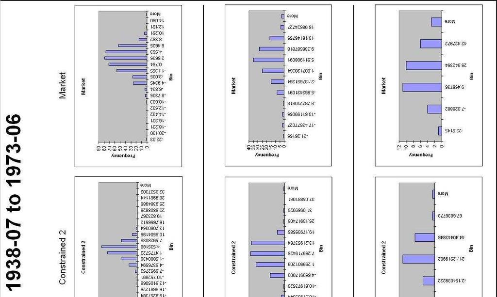
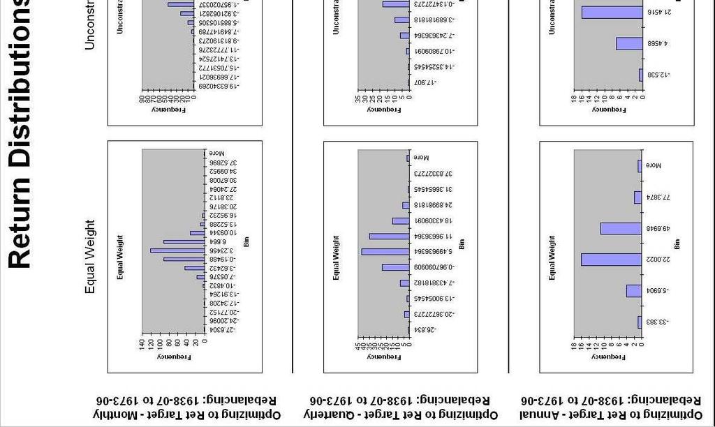
54 APPENDIX A - HISTOGRAMS The following pages include histograms to provide a visual confirmation of the return distributions reported in the results text and figures above. 54

55 55

56 56

57 57

58 58

59 59

60 60