ECMB02F -- Problem Set 2 Solutions

Transcription

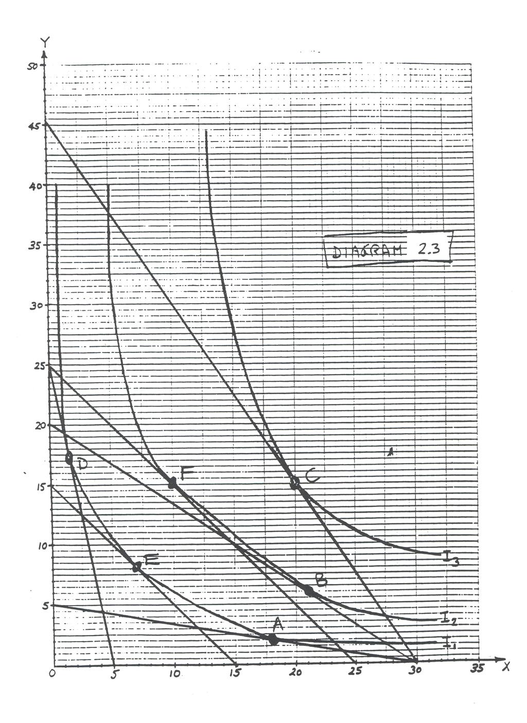
1 1 ECMB02F -- Problem Set 2 Solutions 1. See Nicholson 2a) If P F = 2, P H = 2, the budget line must have a slope of -P F /P H or -1. This means that the only points that matter for this part of the problem are E, H, and K (because these are the only points that lie at the tangency between the indifference curves and budget lines with slopes of -1) (note that all other points are not relevant to this part of the problem). At point E, we get the income one of three ways: by costing out point E, which has F=30 and H=17 ($2x30 + $2x17 = $94); by using the F-intercept for the budget line that has slope -1 and is tangent to the indifference curve at point E (that intercept is 47, so I = P F times the intercept = $2 x 47 = $94); or by using the H-intercept for the budget line (again 47, so I = P H x intercept= $94). Similarly, the income at point H is $120 and the income at point K is $150. So the Engel curve is: Income Amount of Food Again, if P F = 3, P H = 2, the budget line must have a slope of -P F /P H or -3/2. This means that the only points that matter for this part of the problem are B, D, G, and J (because these are the only points that lie at the tangency between the indifference curves and budget lines with slopes of -3/2). Using the techniques discussed earlier when P F =P H =2, we get income at these three points either by costing out the points, or by referring to the intercepts. The income at points B, D, G, and J is 90, 120, 150, and 180. so the Engel curve for food is: Income Amount of Food and the Engel curve for housing is: Income Amount of Housing You may draw the three Engel curves for yourself. b) If I = 360, P F = 6, the budget line must have an F-intercept of 60. This means that the only points that matter for this part of the problem are C, F, H, and J (because these are the only points that lie at the tangency between the indifference curves and budget lines having an F- intercept of 60) (note again that all other points are not relevant to this part of the problem). At all these points we can get the price of housing most easily by dividing 360 by the H-intercept of the budget line (since H-intercept = I/P H, then P H = I divided by the H-intercept) (you could also use the equation P H H + P F F = I at each point, but this is harder). Thus the P H associated

2 2 with point C is 360/15 = 24. Similarly, P H at point F is 360/30 = 12, P H at point H is 360/60 = 6, and P H at point J is 360/90 = 4. So the demand curve is: Price of Housing Amount of Housing Now, if P F = 6 and U is held constant on the I 2 indifference curve, then the only points that matter for this part of the problem are F, E, and D (because these are the only points that lie on the indifference curve I 2 ). We get P H by finding the slope of the three budget lines and setting this equal to -P F /P H = -6/P H. Using this technique, P H is 12 at point F, 6 at point E, and 4 at point D. The compensated demand curve for housing (holding U=I 2 ) is: Price of Housing Amount of Housing Again, I will let you sketch the two demand curves. They are related because they cross at P H = 12. This occurs because the budget lines are the same here (because the uncompensated budget curve at this price hits the indifference curve I 2 so no compensation is needed to stay on I 2 ). c) If I = 120, P H = 2, the budget line must have an H-intercept of 60. This means that the only points that matter for this part of the problem are A, D, and H. At all these points we can get the price of food most easily by dividing 120 by the F-intercept of the budget line. Thus the P F associated with point A is 120/20 = 6, P F at point D is 120/40 = 3, and P F at point H is 120/60 = 2. So the demand curve is: Price of Food Amount of Food d) From the information we have so far, housing is normal since increases in income (prices held constant) always increase the consumption of housing. But food is sometimes inferior, since the second Engel curve in part a does sometimes reduce their consumption of food when income rises (in real life food is a normal good, but you are asked to use the points given here). Neither good is a Giffen good, since the demand curves all slope the "right" way. e) The relevant points are on the diagram in the problem set. When I = 300, P H = 4, the budget lines have an H-intercept of 75. The rise in P F from 4 to 6 moves us from K to G, a fall in the consumption of food of 21. The substitution effect moves us from point K to point J, a fall in the consumption of food of 23, while the income effect moves us from point J to point G, a rise in the consumption of food of 2 (food is inferior in this part of the utility function). The substitution effect looks only at the effect of the change in relative prices, holding utility unchanged. It does this by (in this case) raising the consumer's income so as to stay on the same indifference curve, and thus ignore the fact that an increase in the price of food not only changes relative prices but also makes us worse off. The income effect focuses on the effect of a price change on purchasing power by holding prices constant (at the new price level) and considering

3 3 only the effect of the price change on the consumer's ability to purchase goods. In this case, to keep the consumer on the initial indifference curve I 4 when P F rises to 6, we must enable the consumer to buy point J. This can occur only if the consumer's income is raised to 360. Thus income must rise by 60 to compensate for the increase in the price of food. f) When I = 120 P F = 2, the budget lines have an F-intercept of 60. The fall in P H from 4 to 4/3 moves us from F to J, a rise in the consumption of housing of 48. The substitution effect moves us from point F to point D, a rise in the consumption of housing of 18, while the income effect moves us from point D to point J, a rise in the consumption of housing of 30. In this case, to keep the consumer on the initial indifference curve I 2 when P H falls to 4/3, we must enable the consumer to buy point D. This can occur only if the consumer's income is lowered to 80. Thus income must fall by 40 to compensate for the reduction in the price of food. g) Changes in prices have no effect on the indifference curves. Changes in prices do affect which point on the indifference curve is chosen, but not the location and shape of the indifference curves themselves. 3. I have attached a copy of my diagram with the relevant budget lines drawn in. Of course, since the exact point of tangency is hard to see, there may be a slight difference between my answers and yours. a) When I = 90 and P X = 3, the budget lines all have to have an X-intercept equal to I/P X = 30. To get the demand curve, you must then draw budget lines from that intercept that are tangent to the three indifference curves. These budget lines are tangent at points I have labelled as A, B, and C on my diagram. You can find the price of Y by dividing income (90) by the Y-intercept, or by determining the amount of X and Y at each of the three points (A, B, and C) and solving the equation P X X + P Y Y = I, or 3X + P Y Y = 90. Point A has X=18, Y=2, so the equation is P Y = 90, or P Y = 18. Alternatively, the Y- intercept of the budget line is 5, so P Y = 90/5 = 18. Point B has X=21, Y=6; the Y-intercept of the budget line is 20, so P Y = 90/20 = 4.5. Point C has X=20, Y=15; the Y-intercept of the budget line is 45, so P Y = 90/45 = 2. Thus the demand curve is: Price of Y Amount of Y b) When I = 50 and P Y = 2, the Y-intercept must be 25. When P X is 10, the X-intercept is 5, and the budget line as drawn is tangent to the indifference curve I 1 at point D, where 1.5 units of X is consumed. When P X is 2, the X-intercept is 25, and the budget line as drawn is tangent to the indifference curve I 2 at point F, where 10 units of X is consumed. To get the income and substitution effects, we draw a new budget line with the new price ratio (1/1) that is just tangent to the first indifference curve. This budget line is tangent at point E, where 7 units of X are consumed. Thus the substitution effect shifts consumption from point D to point E, increasing the consumption of X by 5.5 units. The income effect shifts consumption from point E to point F, increasing consumption by 3 units. To compensate for the rise in income, we have to shift the new budget line inwards. That shift reduces both X and Y-intercepts from 25 to 15, and thus is a

4

5 5 reduction in income of 20. Thus the effect of the price of X is to increase real income by 20 (because a reduction in income of 20 shifts the consumer back onto the original indifference curve). 4. This is a Cobb-Douglas utility function. As we have seen, we can use the convenient trick that the consumer spends a constant share of income on each commodity. Since α = β, so the consumer spends half the income on X and half on Y. a) income = 120, P X =P Y =1, so X = 60, Y = 60, U = 3600 b) The tax raises P X to 2, so X = 30, Y = 60, U = The government revenue is $1 on each unit of X, or $30. c) Call the lump sum tax L. After the tax, the consumer's income is L Because the tax leaves prices unchanged, P X =P Y =1. The consumer spends half the income on each good, so X = Y = 0.5(120-L) We want to choose L so that utility is the same as in part b. Thus: U = [0.5(120-L)][0.5(120-L)] = 1800 so 0.5(120-L) = /5 = so L = 84.86, or L = Because the lump sum tax raise $5.14 more than the sales tax, but leaves the consumer no worse off, we can call $5.14 the efficiency loss (or "excess burden") associated with the commodity tax. d) If the lump sum tax is $30, then income is 90, and X = Y = 45 Thus U = 45 2 = Clearly, utility is higher than in part b e) Now the consumer spends 2/3 of his income on X and 1/3 on Y Repeating the problem: part a) X = 80, Y = 40, U = part b) X = 40, Y = 40, U = 40, Revenue = $40 part c) X = (2/3)(120-L) Y = (1/3)(120-L) and we to choose L so that U = 40 Thus [(2/3)(120-L)] 2/3 [(1/3)(120-L)] 1/3 = 40 or (2/3) 2/3 (1/3) 1/3 (120-L) = 40 or (.7631)(.6934)(120-L) = 40 or L = so L = Because the lump sum tax raise $4.41 more than the sales tax, but leaves the consumer no worse off, we can call $4.41 the "excess burden". Finally, if the lump sum tax is instead set at $40, then income is $80, and the Cobb-Douglas rule (that the consumer spends 2/3 of income on X) means that X = and Y = Thus U = / /3 = This is clearly more than 40, so the lump sum tax that yields the same revenue clearly leaves the consumer better off than the commodity tax. f) The problem is that there is not really a practical way to assess a true lump sum tax. An equal tax per person would do the job, but it would hardly be progressive. Any tax conditioned on income also depends on work effort and education and investment all kinds of other behaviour that can vary after the tax is applied (which means that the tax is no longer lump sum). 5a) By Lagrangian multiplier, we set L = x 3 y + λ (I-P x x-5y) To maximize we set L/ x = 3x 2 y - λp X = 0 so 3x 2 y = λp X L/ y = x 3-5λ = 0 so x 3 = 5λ L/ λ = I-P X x-5y = 0

6 6 Dividing the first equation by the second, we get 3y/x = P X /5 or y/x = P X /15 or 5y = P X x/3 We can thus plug 5y into the third equation to get I - P X x - P X x/3 = I - (4/3)P X x = 0, and this solves simply to x = (3/4)I/P X since I = 60, x = 45/P X The overall effect of a change in the price of x is dx/dp X = -45/P 2 X which is dx/dp X = -5 when P X = 3. We know that the income effect is given by - x(dx/di), and clearly dx/di = (3/4)/P X = 3/(4P X ), so when P X = 3 and I = 60, the income effect is -15(1/4) = Since the overall effect is -5, the substitution effect must be b) We know that x = 15, y = 3, so that U = (15 3 )3 = Holding utility constant (which is what we must do to find the compensated demand curve) gives us x 3 y = x and y change along this indifference curve so as set the MRS equal to the price ratio. MRS = ( U/ x)/( U/ y) = 3x 2 y/x 3 = 3y/x If we set this equal to the price ratio, we get 3y/x = P x /P y = P x /5 or y = (P x x/15) Plug this into the equation for the indifference curve and we get x 3 y = x 4 P x /15 = or x 4 = /P x or x = /P.25 x = P -.25 x which is the compensated demand. Taking the derivative of x should give us the substitution effect: dx/dp x = -.25( P x ) = P x Evaluating this expression at P x = 3 gives us dx/dp x = c) In part a, we found that the demand curve was x = 45/P X. Clearly, this does not change when P Y changes. This result is hardly unusual, since it would occur whenever two goods were neither substitutes nor complements. d) By Lagrangian multiplier, we set L = x 1/2 + y 1/2 + λ(i - P x x - 2y) To maximize we set L/ x = (1/2)x -1/2 - P x λ = 0 so x -1/2 = 2 P x λ L/ K = (1/2)y -1/2-2λ = 0 so y -1/2 = 4λ L/ λ = I - P x x - 2y = 0 Dividing the first equation by the second, we get x -1/2 /y -1/2 = P x /2 or y 1/2 /x 1/2 = P x /2 or y/x = P 2 x /4. We can thus plug y = (P 2 x /4)x into the third equation to get I - P x x - (P 2 x /2)x = 0, or x = I/[P x + (P 2 x /2)] = 60/[P x + (P 2 x /2)] Now, the overall effect of a change in the price of x is dx/dp X = -60(1 + P X )/[P x + (P 2 x /2)] 2 which is dx/dp X = -60(4)/56.25 = when P X = 3. We know that the income effect is given by - x(dx/di), and clearly dx/di = 1/[P x + (P 2 x /2)], so when P X = 3 and I = 60, the income effect is -8(1/7.5) = Since the overall effect is , the substitution effect must be e) By Lagrangian multiplier, we set L = (x -1 + y -1 ) -1 + λ(i - P x x - P y y) To maximize we set L/ x = (-1)(x -1 + y -1 ) -2 (-1)x -2 - P x λ = 0 so (x -1 + y -1 ) -2 x -2 = P x λ L/ y = (-1)(x -1 + y -1 ) -2 (-1)y -2 - P y λ = 0 so (x -1 + y -1 ) -2 y -2 = P y λ L/ λ = I - P x x - P y y = 0 Dividing the first equation by the second, we get x -2 /y -2 = P x /P y or y 2 /x 2 = P x /P y or y/x = P.5.5 x /P y We can thus plug P y y = (P x P y ).5 x into the third equation to get I - P x x - (P x P y ).5 x = 0, or x = I/[P x + (P x P y ).5 ] = 150/[P x + 3(P x ).5 ], which is the demand curve. The overall effect of a change in the price of x is dx/dp X = -150( P -.5 X )/[P x + 3P.5 x ] 2 which is dx/dp X = -150(1.75)/100 = when P X = 4 We know that the income effect is given by - x(dx/di),

7 and clearly -xdx/di = -x/[p x + (P x P y ).5 ], so when P X = 4, x = 15, and the income effect is - 15/10 = Since the overall effect is , the substitution effect must be