Journal of College Teaching & Learning February 2007 Volume 4, Number 2 ABSTRACT

Transcription

1 How To Teach Hicksian Compensation And Duality Using A Spreadsheet Optimizer Satyajit Ghosh, ( ghoshs1@scranton.edu), University of Scranton Sarah Ghosh, University of Scranton ABSTRACT Principle of duality and numerical calculation of income and substitution effects under Hicksian Compensation are often left out of intermediate microeconomics courses because they require a rigorous calculus based analysis. But these topics are critically important for understanding consumer behavior. In this paper we use excel solver- a spreadsheet optimizer to demonstrate how these topics can be taught in an undergraduate economics class with appropriate rigor but without using calculus. We also demonstrate how our methodology can be applied to Slutsky Compensation and to complex utility functions. INTRODUCTION I ndifference curve analysis and decomposition of substitution and income effects occupy a major part of any intermediate microeconomics course. However, the majority of the undergraduate textbooks and consequently, most instructors rely solely on graphical analysis to explain the decomposition of the effect of a price change into substitution and income effects. Numerical examples and exercises are often used but they do not provide students with a complete understanding of the analytical methods, since a comprehensive quantitative analysis requires calculus based approach such as the Lagrangean multiplier method which is usually beyond the scope of intermediate courses and textbooks. 1 Most undergraduate courses also leave out the important topic of duality in consumer behavior (which is a principal area of discussion in any graduate course) mostly because it tends to be analytically difficult. However, very few students who take an intermediate microeconomics course pursue graduate studies in economics. This paper is motivated by the need for covering these topics with appropriate rigor in an undergraduate intermediate microeconomics course. However, most undergraduate students in economics and business are not required to take calculus at a level that can make them proficient in learning these topics quantitatively. Fortunately, at least over the past ten years we have witnessed an increased emphasis on computer literacy and use of spreadsheet in undergraduate curriculum across the nation. The paper is written to develop a teaching tool that uses the strength of the computer skills of our undergraduate students in a way to compensate for the deficiency in rigorous mathematical analysis. The purpose of this paper is to develop a simple spreadsheet based approach to discuss duality and analyze income and substitution effects. It is easy to use in an undergraduate class and is capable of providing a very useful insight in the discussion of consumer behavior. Instructors who use a comprehensive mathematical analysis of the subject matter in advanced undergraduate courses can also use this methodology to supplement their teaching. It should, however, be noted that we focus on the process of compensation and the concept of duality but we do not attempt to derive the exact functional forms of Marshallian or Hicksian demand functions and expenditure or indirect utility functions. Such derivations, as noted before, require advanced calculus and are beyond the scope of undergraduate intermediate courses in microeconomics. The plan of this paper is as follows. In section 2 we provide the traditional graphical analysis of the decomposition of income and substitution effects. This also serves as a basis for our spreadsheet application. In section 3 we discuss the concept of duality that helps us to develop the spreadsheet application and in section 4 we develop a numerical example to illustrate how a spreadsheet based optimizing routine such as the Excel-Solver can be used to analyze income and substitution effects. In section 5 we briefly suggest additional applications and generalizations of our approach. Concluding remarks are made in section 6. 65

2 BACKGROUND AND GRAPHICAL ANALYSIS An individual consumer s optimal purchasing decision is traditionally viewed as one of maximization of utility provided the consumer stays within the budget constraint, i.e., as long as she does not spend more than her income. In order to carry out a graphical analysis we assume that the consumer buys only two goods, x and y. Prices of the products are p x and p y and are outside our consumer s control. The consumer has a fixed income of $I. Algebraically, the consumer s optimizing problem is written as Maximize U= U(x, y) (1) Subject to p x x +p y y I (2) The consumer chooses x and y to maximize utility. Figure 1 describes the familiar graph of utility maximization, which is also used to analyze income and substitution effects. A set of standard convex indifference curves as shown in figure 1 depicts our consumer s preference structure. The line AB shows the initial budget line along which the budget constraint (2) is satisfied as equality. The initial utility maximizing point is E where the consumer consumes x 1 and y 1 amounts of the products and attains the utility level u 2. Figure 1: Substitution And Income Effects C A y 2 F y 3 y 1 G u 1 E u 2 x 3 B D B x 2 x 1 AB: Initial Budget Line; AB : Budget Line after an increase in price of x. CD: Compensated Budget Line after Hicksian Compensation. Substitution Effect: (x 2 x 1 ); Income Effect: (x 3 x 2 ). Price Effect: (x 3 x 2 ) We now consider the impact of an increase in price of x on the optimal purchase plan of the consumer. In particular we focus on the consumption of the product x itself. After an increase in price of x the budget line swings to the steeper line AB and the consumer s optimal bundle drops to G where the consumer buys x 3 and y 3 amounts and attains a lower level of utility u 1. The change in consumption of x, (x 3 x 1 ) measures the price effect. 66

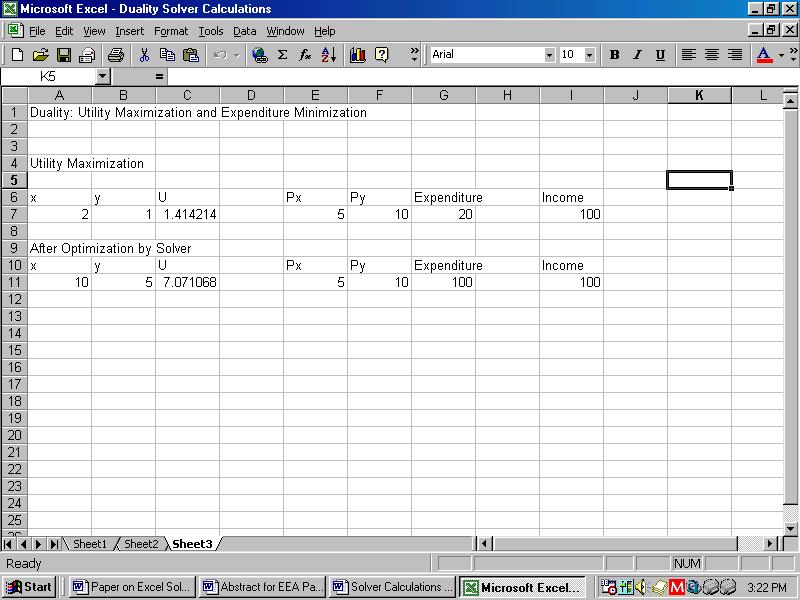
3 However, this change in consumption subsumes a substitution effect and an income effect. In order to disentangle the substitution and income effects we use Hicksian Compensation. 2 We compensate the consumer for the increase in price of x by providing her just enough additional income so that she can stay on the same indifference curve, u 2. To this effect we draw the compensated budget line CD that is parallel to the new (post price rise) budget line AB and tangent to the initial indifference curve with utility level u 2 at point F. This gives rise to an intermediate equilibrium position at F. Consumer s optimal bundle changes from E to F where she buys x 2 and y 2 amounts of the two products. The movement from bundle E to F is thus due to the substitution effect and in terms of x it is measured by (x 2 x 1 ). Furthermore the bundle E defines ordinary or Marshallian demands for the goods while the bundle F defines the compensated or Hicksian demands. The movement from F to G captures the income effect of an increase in price of x and in terms of x it is measured by (x 3 x 2 ). The substitution and income effects add up to the price effect. It is clear that at this point a numerical example can greatly help student understanding of these somewhat abstract concepts of substitution and income effects. But since the use of calculus based optimization tool such as the Lagrangean Multiplier method is typically beyond the scope of most Intermediate courses and texts, the numerical examples that are developed often seem to be ad hoc. However, spreadsheet based optimizing programs such as Excel-Solver can provide a comprehensive illustration of the decomposition of substitution and income effects and can enhance student understanding by focusing on the analytical aspects of the process of Hicksian Compensation. Since our spreadsheet application uses the dual problem of expenditure minimization, in the next section we briefly discuss some results from the theory of duality. THE DUAL PROBLEM AND AN EXCEL-SOLVER APPLICATION Consider the following dual problem for utility maximization, as described in equations (1) and (2). A representative consumer s choice problem can be equivalently viewed as one of expenditure minimization where the individual intends to buy a particular class of product bundles at the lowest possible cost. In other words the consumer chooses the amounts of x and y in order to Minimize E = p x x + p y y (3) Subject to U(x, y) = U (4) where U is the fixed level of utility associated with the indifference curve and the equivalent bundles on the curve that the individual wants to purchase. In the theory of consumer behavior the principle of duality provides the important insight that the solutions from the expenditure minimization problem are identical to the solutions from the utility maximization problem if the optimal level of utility obtained from the utility maximization problem (equations (1) and (2)) is the same as the utility constraint U in equation (4) of the expenditure minimization problem. We can use the duality results to demonstrate the decomposition of price effect into substitution and income effects. Unfortunately, while graduate textbooks provide extensive discussions of principle of duality, only a handful of undergraduate texts pay any attention to this topic. 3 Discussion of duality often tends to be analytically challenging but simple spreadsheet exercises can demonstrate the basic results. Using Excel s optimizing routine Solver we now construct a simple spreadsheet based example to illustrate the basic principles of duality. This example will also serve as the foundation for our discussion of Hicksian compensation. An Example Using Excel Solver Consider the simple Cobb Douglas utility function 4 U = x 1/2 y 1/2. Prices and income are: p x = $5, p y = $10 and I = $100. First, we want to determine the initial equilibrium point when the consumer wants to maximize utility subject to the budget constraint, 5x + 10y = 100. We create an excel worksheet as in Exhibit 1A. We focus on rows 6 67

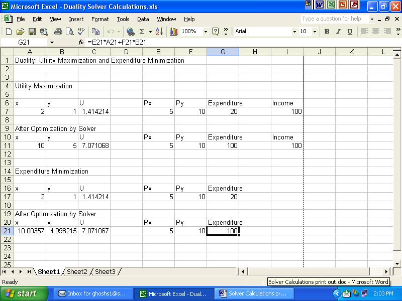
4 and 7. We enter values and formulas in cells in row 7. Since we are interested in utility maximizing values of x and y, we begin by entering arbitrary values, 2 and 1 for x and y in cells A7 and B7 respectively. Values of prices and income are entered in E7, F7 and I7. We now enter the two formulas of the utility function and expenditure that are needed for both utility maximization and expenditure minimization. In cell C7 we enter the formula for the utility function by typing = (A7)^.5*(B7)^.5. In cell G7 we enter the formula for expenditure (p x x +p y y) by typing = E7*A7 + F7*B7. We are now ready to use the optimizing program, solver to determine the initial utility maximizing bundle. From Excel s tools menu we invoke Solver. In the Solver window we specify the solver parameters for the problem at hand. We prompt the solver to maximize utility by entering $C$7 in the Set Target Cell window and then click on the button, Equal To: Max. We want to find values of x and y (cells A7, B7) that can maximize utility. So in the window, By Changing Cells we enter $A$7:$B$7. Finally, we specify the budget constraint (Expenditure= Income) by entering in the Subject to the Constraints window the cell addresses that define our constraint: $G$7=$I$7. Exhibit 1A shows how the utility maximizing problem is defined. In order to determine the optimal solution to this problem we click on Solve and when prompted, we click on Keep Solver Solution. The optimal values are shown in row 11 of exhibit 1B. Specifically, the optimal values of x and y (10 and 5 respectively, shown in cells A11 and B11) define the Marshallian demands for the goods. 5 Resulting optimal value of utility, U*= is in cell C11. We now turn to the dual problem of expenditure minimization. First we define an expenditure minimizing problem in rows 16 and 17 and the accompanying Solver window in Exhibit 1C. Once again, we begin with arbitrary values of 2 and 1 for x and y. The formula for the utility function, U = x 1/2 y 1/2, is entered in C17. Values of the prices of x and y are entered in E17 and F17 respectively. The formula for expenditure, p x x + p y y or 5x+10y is entered in G17. The goal is now to find the values of x and y that can minimize consumer s expenditure but can attain a given utility level. In the Solver window we specify the parameters for this expenditure minimization problem. The Target Cell is now G17, the cell address for expenditure. We click on the Min button to minimize expenditure. The decision variables are x and y. So we want to change cells A17 through B17. Finally, to illustrate the principle of duality we define the constraint to be the optimal level of utility, U*= attained in the previous utility maximizing problem. Thus in the Subject to the Constraints window we enter $C$17= The optimized values are shown in row 21 of Exhibit 2. For convenience, the complete solutions of the utility maximizing and expenditure minimizing problems are shown in the spreadsheet of Exhibit 2. From the results reported in row 11 and row 21, we observe that the optimal value of expenditure for the expenditure minimization problem is the same as the value of income in the budget constraint of the utility maximization problem and that, with some rounding up, the optimal amounts of x and y are identical under utility maximization and expenditure minimization. This simple spreadsheet application provides us some very important identities in principle of duality. In order to illustrate the results from duality theory, denote the maximum value of utility obtained in the utility maximization problem as U* (p x, p y, I), the Indirect Utility function and the minimum value of expenditure obtained in the expenditure minimization problem as the Expenditure function, E(p x,p y, U). The utility maximizing amounts of x and y are ordinary or Marshallian demands, x m (p x, p y, I) and y m (p x, p y, I). The expenditure minimizing values of x and y are compensated or Hicksian demands, x h (p x, p y, U) and y h (p x, p y, U). The results of rows 11 and 21 can now help us illustrate the following important identities: E(p x, p y, U*) I (5) x m (p x, p y, I) x h (p x, p y, U*) and y m (p x, p y, I) y h (p x, p y, U*) (6) x h (p x, p y, U) x m (p x, p y, E(p x,p y, U)) and y h (p x, p y, U) y m (p x, p y, E(p x,p y, U) (7) (5) implies that the minimum expenditure necessary to attain utility U* (p x, p y, I) is I. (6) and (7) illustrate the relationships between Marshallian and Hicksian demands. (6) implies that the Marshallian demand at income I is the same as Hicksian demand at utility U* (p x, p y, I) while (7) demonstrates that the Hicksian demand at utility U is the same as the Marshallian demand at income E(p x,p y, U) 6. 68

5 The spreadsheet based optimizing example and the above duality results are particularly important because on the one hand they serve as an introduction to the principle of duality and on the other they provide the background for a numerical example to demonstrate the income and substitution effects. 7 In the following section we develop a spreadsheet based application to determine the income and substitution effects of a price increase. AN EXCEL SOLVER APPLICATION TO DETERMINE INCOME AND SUBSTITUTION EFFECTS Using the principle of duality we can analyze the decomposition of income and substitution effects in terms of a combination of utility maximizing and expenditure minimizing problems. The initial equilibrium point, E in figure 1 can be determined as the solution to a utility maximizing problem where the initial set of prices and the original income level define the budget constraint (shown by AB). The consumer attains the utility level u 2. Now, the process of Hicksian Compensation can be considered as one of expenditure minimization under the new set of prices where the utility level u 2 defines the constraint. As a result, the optimal expenditure level determines the compensated budget line CD and the intermediate equilibrium point F is obtained as the solution to the expenditure minimizing problem. Finally, the equilibrium point G is determined as the optimal solution to a utility maximizing problem where the budget constraint (shown by AB ) is defined by the original income level and the new set of prices. We can now use the spreadsheet based optimizing routine Excel-Solver to extend and modify our example from the previous section to illustrate the decomposition of income and substitution effects. Besides providing an example, it can greatly enhance student understanding of the process of compensation and income and substitution effects by focusing on the analytical structure of the method of compensation. We consider the same utility function U = x 1/2 y 1/2. Initial prices and income are: p x = $5, p y = $10 and I = $100. First, we want to determine the initial equilibrium point (E in figure 1) when the consumer wants to maximize utility subject to the budget constraint, 5x + 10y = 100 i.e., expenditure = income. It is the same utility maximizing problem that we have solved in the duality example. We copy the optimizing problem from Exhibit 2 and create exhibit 3. For our convenience Exhibit 3 shows all relevant calculations. Solution to the initial utility maximizing problem is shown in row 11 of Exhibit 3. The optimal values of x, y and utility are determined to be 10, 5 and respectively. Now, the price of x increases to $10 while price of y and income remain unchanged. Following the same steps as before, we use the Solver to calculate the new utility maximization position (G in figure 1) after redefining the budget constraint to reflect the new higher price of x. The optimal values are displayed in row 16 of Exhibit 3. The price effect of a change in price of x is determined to be the change in the consumption of x, i.e., 5-10 = -5. Next, we turn to decomposition of price effect into substitution and income effects. As explained earlier, the compensation mechanism can be viewed as an expenditure-minimizing problem. The minimization problem is defined in rows 19, 20 of Exhibit 3. Once again, we begin with arbitrary values of 2 and 1 for x and y. The formula for the utility function is entered in C20. Values of the (new higher) price of x and the price of y are entered in E20 and F20 respectively. The formula for the Expenditure function, now defined as 10x+10y is entered in G20. The goal is now to find the values of x and y (in bundle F of figure 1) that can minimize consumer s expenditure but can attain the original indifference curve with utility level calculated to be In the Solver window we specify the parameters for this expenditure minimization problem. The Target Cell is now G20, the cell address for the expenditure function. We click on the Min button to minimize expenditure. The decision variables are x and y. Finally, the constraint is defined to be the level of utility attained in the first utility maximizing bundle (E in figure 2). Thus in the Subject to the Constraints window we enter $C$20= The optimized values are shown in row 24 of Exhibit 3. Thus the intermediate equilibrium position is determined to be x = 7.07, y = The substitution effect, in terms of x is calculated to be ( )= and the income effect is calculated to be (5-7.07)= Since, between the intermediate equilibrium bundle F and the final bundle G the level of income falls and as a result the levels of consumption of x and y also fall, x and y are determined to be normal goods. The substitution and income effects add up to the price effect of 5. Furthermore, the level of 69

6 Income Compensation can be calculated as the difference between the optimal value of expenditure under the expenditure minimizing problem and the original level of income, i.e., ( )= ADDITIONAL APPLICATIONS AND GENERALIZATIONS In the previous section we developed a procedure to demonstrate the decomposition of the effect of a price increase into income and substitution effects using a simple Cobb-Douglas utility function. Our procedure, however, is general enough so that it can be used for demonstrating the Slutsky Compensation, and also can be used to handle more general utility functions. In this section we demonstrate three additional applications. To conserve space we have not included the spreadsheets for these additional applications. They can be obtained from us on request. The most widely used method of income compensation and decomposition of income and substitution effects is the method of Hicksian Compensation that we discussed in section 4. But some instructors may like to use the alternative Slutsky Compensation, which compensates the consumer after a price increase by providing her additional income so that she can purchase the same initial bundle (prior to price increase) even after a price increase. Thus in terms of figure 1, the compensated budget line under Slutsky Compensation is parallel to AB but passes through point E. As a result the intermediate equilibrium point must lie on an indifference curve that is higher than u 2. To illustrate Slutsky Compensation continue with the same utility function as in the previous section. The initial and final bundles, E and G are the same as before (see rows 11, 16 and 17 of Exhibit 3). To determine the intermediate equilibrium point F, first note that the individual must be compensated such that she can buy bundle E (x= 10, y=5) after the price increase. Thus her new income should be I = 10*10+10*5 = $150. The amount of income compensation is $50. We can now use solver to maximize utility by changing the values of x and y with a new constraint, 10*x+10*y = 150 (i.e., expenditure = newly compensated income). The optimal values for x, y and U are found to be 7.5, 7.5 and 7.5. These define the intermediate equilibrium point F. In terms of x, both substitution and income effects are 2.5. A quick comparison of the optimal utility value of 7.5 with U = 7.07 (cell c24 in exhibit 3) under Hicksian compensation can be used by instructors to discuss the concept of overcompensation under Slutsky Compensation. The Solver based method that we demonstrated in section 4 to illustrate Hicksian Compensation is not limited to the simple Cobb Douglas utility function that we used and also not just to price increase. Here we provide two additional examples of more general utility functions when price of x decreases. First consider a more general Cobb Douglas utility function, U = x 2 y. Suppose that the initial prices and income are given to be p x = $20, p y =$10 and I = $300. Price of x then declines to $10. Using the solver based method described in the previous section, it can be readily verified that the initial and final equilibrium bundles are (x 1 = 10, y 1 = 10) and (x 3 = 20, y 3 = 10) respectively. The intermediate equilibrium bundle after Hicksian Compensation can be obtained as (x 2 = 12.6, y 2 = 6.3). Thus in terms of x the magnitudes of the substitution and income effects are calculated as 2.6 and 7.4 respectively. Finally, consider the following example of a CES utility function, U = (x -1 + y -1 ) -1 = xy/(x+y). Price of x falls from $4 to $2 while p y and I remain unchanged at $1 and $30 respectively. Following the same solver based methodology we can determine the initial and final utility maximizing bundles as well as the intermediate equilibrium bundle after conducting a Hicksian Compensation. The initial and final bundles can be determined as (x 1 = 5, y 1 = 10) and (x 3 = 8.79, y 3 = 12.43) respectively. After Hicksian Compensation the intermediate equilibrium bundle is obtained as (x 2 = 5.69, y 2 = 8.05). Thus in terms of x the magnitudes of the substitution and income effects are found to be.69 and 3.10 respectively. CONCLUSION We have shown how using Excel-Solver, a spreadsheet based optimization routine, we can teach Substitution and Income Effects in undergraduate intermediate microeconomics class. As we have shown, it can greatly enhance the traditional graphical exposition. The main advantage of this spreadsheet based optimizing example is that in every step of this example we focus on the objective function and the constraint. Thus it can improve the understanding of 70

7 the analytical structure of Hicksian compensation and the associated concepts of income and substitution effects. Instructors using a calculus based approach can also use this methodology to supplement their discussion. Furthermore, through this approach students can learn the principle of duality, which is a central topic in a graduate course in microeconomic theory but is often ignored in undergraduate classes. After learning this solver application students can apply the methodology for more complex utility functions and also to other areas of optimizing economic decisions such as cost minimization, profit maximization among others. ENDNOTES 1. Only a handful of Intermediate texts, such as Besanko and Braeutigam (2002), Katz and Rosen (1997), Nicholson (1998) and a few others discuss the Lagrangean Multiplier method. However, a comprehensive calculus based treatment of substitution and income effects is still beyond the scope of these texts. They all provide excellent graphical analysis of the topic. 2. In this paper we focus on Hicksian Compensation, which is analytically superior to the alternative of Slutsky Compensation. Most intermediate texts also discuss only Hicksian Compensation. However, we will briefly touch on the topic of Slutsky Compensation in section Among undergraduate texts Besanko and Braeutigam and particularly Nicholson provide nice discussions on duality. All graduate texts such as Varian (1992) or Kreps (1990) include comprehensive treatment of duality. 4. In section 5 we consider a more general Cobb-Douglas utility function and a Constant Elasticity of Substitution (CES) utility function. 5. As noted before, we are not deriving the functional form of the Marshallian demand function. The spreadsheet calculates the amount demanded given prices and income. Using calculus one can determine the demand function for x and y as x= I/(2p x ) and y=i/(2p y ). Given prices of x and y and income, I the values in A11 and B11 can easily be verified as Marshallian demands. 6. Again we are focusing on the equality of specific values. 7. Interested students can consult Varian or any other graduate text for analytical treatment of these identities. REFERENCES 1. Besanko, D. and R. Braeutigam Microeconomics: An Integrated Approach. New York: John Wiley and Sons. 2. Katz, M and H. Rosen Microeconomics, 3 rd. Edition. New York: McGraw Hill. 3. Kreps, D A Course in Microeconomic Theory. Princeton: Princeton University Press. 4. Nicholson, W Microeconomic Theory, 7 th. Edition, Fort Worth: Dryden Press. 5. Varian, H Microeconomic Analysis, 3 rd. Edition. New York: W.W. Norton. 71

8 EXHIBIT 1A EXHIBIT 1B 72

9 EXHIBIT 1C EXHIBIT 2 73

10 EXHIBIT 3 74