Sociology 704: Topics in Multivariate Statistics Instructor: Natasha Sarkisian. Binary Logit

Transcription

1 Sociology 704: Topics in Multivariate Statistics Instructor: Natasha Sarkisian Binary Logit Binary models deal with binary (0/1, yes/no) dependent variables. OLS is inappropriate for this kind of dependent variable because we would violate numerous OLS assumptions (e.g., that the dependent variable is quantitative, continuous, and unbounded, or that the error terms should be homoscedastic and normally distributed). Two main types of binary regression models are used most often logit and probit. The two types differ in terms of the assumed variance of the error term, but in practice their results are usually very similar, and the choice between the two is mainly the matter of taste and discipline conventions. We ll mostly focus on logit models. Binary logit and probit models as well as other models we ll discuss this semester are estimated using Maximum Likelihood estimation techniques numerical, iterative techniques that search for a set of parameters with the highest level of the likelihood function (likelihood function tells us how likely it is that we would observe the data in hand for each set of parameters, and in fact what we maximize is the log of this likelihood function). This process is a trial and error process. Logit or probit output includes information on iterations those iterations are the steps in that search process. Sometimes, with complicated models, the computer cannot find that maximum then we get convergence problems. But this never happens with binary logit or probit models. To run logit or probit models in Stata, the dependent variable has to be coded 0/1 -- it cannot be 1 and 2, or anything else. Let s generate a 0/1 variable:. codebook grass -- grass should marijuana be made legal -- type: numeric (byte) label: grass range: [1,2] units: 1 unique values: 2 missing.: 1914/2765 tabulation: Freq. Numeric Label legal not legal gen marijuana=(grass==1) if grass~=. (1914 missing values generated). tab marijuana, miss marijuana Freq. Percent Cum , Total 2,

2 . xi: logit marijuana sex educ age childs Iteration 0: log likelihood = Iteration 1: log likelihood = Iteration 2: log likelihood = Iteration 3: log likelihood = Logistic regression Number of obs = 845 LR chi2(4) = Prob > chi2 = Log likelihood = Pseudo R2 = marijuana Coef. Std. Err. z P> z [95% Conf. Interval] sex educ age childs _cons Basic interpretation: Women are less likely than men to support legalization of marijuana. The effect of education is not statistically significant. Those who are older and have more children are less likely to support legalization. Divorced people are more likely than married people to support legalization. *Same with probit. probit marijuana sex educ age childs Iteration 0: log likelihood = Iteration 1: log likelihood = Iteration 2: log likelihood = Iteration 3: log likelihood = Probit regression Number of obs = 845 LR chi2(4) = Prob > chi2 = Log likelihood = Pseudo R2 = marijuana Coef. Std. Err. z P> z [95% Conf. Interval] sex educ age childs _cons Goodness of fit. estat gof Logistic model for marijuana, goodness-of-fit test number of observations = 845 number of covariate patterns = 748 Pearson chi2(743) = Prob > chi2 = The high p-value indicates that model fits well (there is no significant discrepancy between observed and predicted frequencies). But: this is a chisquare test that compares observed and predicted outcomes in cells defined by 2

3 covariate patterns all possible combinations of independent variables. In this case, there are 770 covariate patterns, so it 770 cells for chi-square test, and therefore very few cases per cell. Not a good situation for a chisquare test. Hosmer and Lemeshow suggested an alternative measure that solves the problem of too many covariate patterns. Rather than compare the observed and predicted frequencies in each covariate pattern, they divide the data into ten cells by sorting it according to the predicted probabilities and breaking it into deciles (i.e. the 10% of observations with lowest predicted probabilities form the first group, then next 10% the next group, etc.). This measure of goodness of fit is usually preferred over the Pearson chi-square. Here s how we obtain it:. estat gof, group(10) Logistic model for marijuana, goodness-of-fit test (Table collapsed on quantiles of estimated probabilities) number of observations = 845 number of groups = 10 Hosmer-Lemeshow chi2(8) = Prob > chi2 = Again, the model appears to fit well. If it were not, we could rely on various diagnostics (discussed below) to improve model fit. Other measures of fit can be obtained using fitstat. But first, we need to install it, along with other commands written by Scott Long, the author of our textbook:. net search spost [output omitted] We need spostado from Now let s obtain fit statistics for our last model. fitstat, save Measures of Fit for logit of marijuana Log-Lik Intercept Only: Log-Lik Full Model: D(840): LR(4): Prob > LR: McFadden's R2: McFadden's Adj R2: ML (Cox-Snell) R2: Cragg-Uhler(Nagelkerke) R2: McKelvey & Zavoina's R2: Efron's R2: Variance of y*: Variance of error: Count R2: Adj Count R2: AIC: AIC*n: BIC: BIC': BIC used by Stata: AIC used by Stata: See pp of Long and Freese for details on these measures of fit. McFadden s R2 is what s commonly reported as Pseudo-R2, although that tends to be fairly low. Log likelihood value or deviance (-2LL) are also frequently reported. Examining the ratio of D/df to see how far from 1.0 it is gives us an idea of model fit (here: /840= ). Another very useful measure is BIC based on the differences in BIC between models, we can select a model with a better fit more reliably than based on a 3

4 difference in Pseudo-R2 or even based on lrtest. Here s how we compare model fit using fitstat. We already saved the results of the previous model. Let s say, we consider adding the marital status dummies:. xi: logit marijuana sex age educ childs i.marital i.marital _Imarital_1-5 (naturally coded; _Imarital_1 omitted) Logistic regression Number of obs = 845 LR chi2(8) = Prob > chi2 = Log likelihood = Pseudo R2 = marijuana Coef. Std. Err. z P> z [95% Conf. Interval] sex age educ childs _Imarital_ _Imarital_ _Imarital_ _Imarital_ _cons fitstat, dif Measures of Fit for logit of marijuana Current Saved Difference Model: logit logit N: Log-Lik Intercept Only Log-Lik Full Model D (836) (840) (4) LR (8) (4) (4) Prob > LR McFadden's R McFadden's Adj R ML (Cox-Snell) R Cragg-Uhler(Nagelkerke) R McKelvey & Zavoina's R Efron's R Variance of y* Variance of error Count R Adj Count R AIC AIC*n BIC BIC' BIC used by Stata AIC used by Stata Difference of in BIC' provides strong support for saved model. Note: p-value for difference in LR is only valid if models are nested. This suggests that adding marital status does not add enough to justify adding 4 extra variables. Again, we could consider adding just one dummy, divorced, and that would probably be worth it in terms of model fit. Here s how to interpret the difference in BIC (guidelines from Raftery 1995): 4

5 Note that if the variable you add to the second model changes the number of cases (because of missing data), BIC comparison won t work. E.g., add income:. logit marijuana sex age educ childs rincom98 Logistic regression Number of obs = 599 LR chi2(5) = Prob > chi2 = Log likelihood = Pseudo R2 = marijuana Coef. Std. Err. z P> z [95% Conf. Interval] sex age educ childs rincom _cons fitstat, dif Measures of Fit for logit of marijuana Current Saved Difference Model: logit logit N: N's do not match. To make the comparisons, use the force option. Because our samples are not the same, so it s problematic to compare models. Do not use force option, however such a comparison would not be correct. A better strategy is to limit both models to the same sample:. logit marijuana sex age educ childs if rincom98~=. Logistic regression Number of obs = 599 LR chi2(4) = Prob > chi2 = Log likelihood = Pseudo R2 = marijuana Coef. Std. Err. z P> z [95% Conf. Interval] sex age educ childs _cons fitstat, save 5

6 Measures of Fit for logit of marijuana Log-Lik Intercept Only: Log-Lik Full Model: D(594): LR(4): Prob > LR: McFadden's R2: McFadden's Adj R2: ML (Cox-Snell) R2: Cragg-Uhler(Nagelkerke) R2: McKelvey & Zavoina's R2: Efron's R2: Variance of y*: Variance of error: Count R2: Adj Count R2: AIC: AIC*n: BIC: BIC': BIC used by Stata: AIC used by Stata: logit marijuana sex age educ childs rincom98 Logistic regression Number of obs = 599 LR chi2(5) = Prob > chi2 = Log likelihood = Pseudo R2 = marijuana Coef. Std. Err. z P> z [95% Conf. Interval] sex age educ childs rincom _cons fitstat, dif Measures of Fit for logit of marijuana Current Saved Difference Model: logit logit N: Log-Lik Intercept Only Log-Lik Full Model D (593) (594) 4.728(1) LR (5) (4) 4.728(1) Prob > LR McFadden's R McFadden's Adj R ML (Cox-Snell) R Cragg-Uhler(Nagelkerke) R McKelvey & Zavoina's R Efron's R Variance of y* Variance of error Count R Adj Count R AIC AIC*n BIC BIC' BIC used by Stata AIC used by Stata Difference of in BIC' provides weak support for saved model. Note: p-value for difference in LR is only valid if models are nested. 6

7 It looks like based on BIC we wouldn t add income to the model. Another way to assess model fit is to concentrate on its predictive powers. This is especially important when we plan to use the model for prediction (e.g., we want to predict who would support legalization of marijuana for a sample that does not contain those data but contains all our independent variables). One way to assess predictive power is to look at prediction statistics:. qui logit marijuana sex age educ childs [output omitted]. estat clas Logistic model for marijuana True Classified D ~D Total Total Classified + if predicted Pr(D) >=.5 True D defined as marijuana!= Sensitivity Pr( + D) 23.68% Specificity Pr( - ~D) 91.13% Positive predictive value Pr( D +) 60.00% Negative predictive value Pr(~D -) 68.00% False + rate for true ~D Pr( + ~D) 8.87% False - rate for true D Pr( - D) 76.32% False + rate for classified + Pr(~D +) 40.00% False - rate for classified - Pr( D -) 32.00% Correctly classified 66.86% We can see that our model classified correctly 66.86% of cases. Note that it only classified 120 people out of 845 as supporters of marijuana legalization. The four cells in the table indicate how classification by the model compares to true status of each case. The statistics below reflect the percentage from the table above and indicate predictive success rates and rates of errors. Sensitivity indicates the percentage of cases with Y=1 that we identified correctly, and specificity indicates the percentages of cases with Y=0 that we classified correctly. We can see that our sensitivity is but our specificity is much higher (91.13%). To alter that for a given model, we can change the cutoff point. In this table, the cutoff is 0.5 this means that all observations with predicted probabilities of.5 and above get classified as 1 (i.e. supporters of legalization) and those observations with predicted probabilities below.5 are classified as 0 (against legalization). It appears that most cases have predicted probabilities below.5. Let s try to shift that cutoff to.3:. estat clas, cutoff(.3) Logistic model for marijuana True Classified D ~D Total Total

8 Classified + if predicted Pr(D) >=.3 True D defined as marijuana!= Sensitivity Pr( + D) 79.61% Specificity Pr( - ~D) 39.19% Positive predictive value Pr( D +) 42.38% Negative predictive value Pr(~D -) 77.37% False + rate for true ~D Pr( + ~D) 60.81% False - rate for true D Pr( - D) 20.39% False + rate for classified + Pr(~D +) 57.62% False - rate for classified - Pr( D -) 22.63% Correctly classified 53.73% Now our sensitivity and specificity are more balanced. We can further examine them and then select a cutoff point using the following command that graphs them against each other:. lsens Sensitivity/Specificity Probability cutoff Sensitivity Specificity Looks like the cutoff point of.4 would be close to the point where specificity and sensitivity are equal. But, the selection of the cutoff will depend on what s more important to us correctly identify 0s or 1s, and what type of error is more problematic to us this will depend in the task at hand. Diagnostics for binary logit Before conducting logistic regression, it might be a good idea to check univariate distributions of independent variables and if some deviate substantially from normal and you can easily correct that with a transformation, then try those transformations. Although normality is not required, it may help avoid other problems. Obviously, this does not apply to your dependent variable. Also note that in logistic regression, we do not expect residuals to be normally distributed. 8

9 Further, before conducting multivariate analysis, you should also check the linearity of bivariate relationships (see below). 1. Multicollinearity For multicollinearity, we can again use VIFs. But to obtain them, we need to run a regular OLS regression model with the same variables and then obtain VIFs VIF command doesn t function after logit regression, even though VIF statistics don t depend on the dependent variable but rather on the correlations among the independent ones. So here s what we d do:. qui reg marijuana sex age educ childs _Imarital_3. vif Variable VIF 1/VIF childs age educ sex _Imarital_ Mean VIF Linearity In logistic regression, linearity and additivity in logits is expected (i.e. the relationships are nonlinear, but they should be linear in terms of the log odds). Bivariate graphical examination using lowess helps identify problems:.lowess marijuana age Lowess smoother marijuana age of respondent bandwidth =.8 Note that we should not expect a straight line after all, probability curve is not a straight line. But this can help you spot, for instance, a parabola. In multivariate context, you can use boxtid--don t forget to specify that you are using logit rather then reg when using boxtid, i.e. use:. boxtid logit marijuana sex age educ childs 9

10 3. Additivity You can once again use fitint command to search for interactions; the syntax is. fitint logit marijuana sex age educ childs, twoway(sex age educ childs) factor(sex) Note that interactions as a method to compare two or more groups can be problematic in logit or probit models because the coefficients are scaled according to the differences in residual dispersion. If you are interested in group comparisons, see: Allison, Paul D Comparing Logit and Probit Coefficients Across Groups. Sociological Methods and Research, 28: Hoetker, Glenn Confounded Coefficients: Extending Recent Advances in the Accurate Comparison of Logit and Probit Coefficients Across Groups. Long, Scott Comparing Group Effects in Logit and Probit Models Outliers and influential data points To detect influential observations and outliers, there are a few statistics you can obtain using predict command after logit p xb stdp dbeta deviance dx2 ddeviance hat number residuals rstandard pattern) predicted probability of a positive outcome; the default linear prediction standard error of the linear prediction Pregibon (1981) Delta-Beta influence statistic deviance residual Hosmer and Lemeshow (2000) Delta chi-squared infl. stat. Hosmer and Lemeshow (2000) Delta-D influence statistic Pregibon (1981) leverage sequential number of the covariate pattern Pearson residual (adj. for # sharing covariate pattern) standardized Pearson residual (adj. for # sharing covariate To examine residuals, it is recommended to use standardized Pearson residual that accounts for in-built heteroscedasticity of residuals in the logit model.. logit marijuana sex age educ childs [Output omitted]. predict rstandard, rs (1920 missing values generated) We can plot residuals against the predicted values and examine observations with residuals high in absolute value:. predict prob (option p assumed; Pr(marijuana)) (25 missing values generated). scatter prob rstandard, xline(0) mlabel(id) 10

11 Pr(marijuana) standardized Pearson residual Observations on the far left or far right deserve further examination. Here, we would especially look at 766 and 2189, but also To identify influential observations, we can obtain a number of leverage statistics:. predict dbeta, dbeta (1920 missing values generated). predict hat, hat (1920 missing values generated). predict dx2, dx2 (1920 missing values generated) We can then examine these graphically to identify problematic observations:. scatter dbeta prob, mlabel(id) Pregibon's dbeta Observations 766, 2189 stand out again as the ones with highest values of dbeta Can similarly examine dx2 and hat values 11

12 We can also combine the information about multiple leverage statistics in one plot:. scatter dbeta rs [w=dx2], mfc(white) xline(0) Pregibon's dbeta standardized Pearson residual Again those two observations (we can verify that they are the same ones by using mlabel option). These observations definitely warrant investigation we need to figure out what s special about them and then decide how to deal with them. 5. Error term distribution In terms of the error term distribution, we don t check for it directly (like with heteroscedasticity test in OLS). There is in-built heteroscedasticity in logit models the variance of the error term is the greatest at the predicted probabilities around.5 and the smallest as we approach 0 or 1. But we still should be concerned whether the logit assumptions about the variance of the error term are correct. To test that, we can obtain robust standard error estimates and compare them with the regular standard error estimates. If they are similar, then our logistic results are fine. If they differ a lot, however, we would rather report robust standard errors as they do are correct even in the presence of assumptions violation.. logit marijuana sex age educ childs Logistic regression Number of obs = 845 LR chi2(4) = Prob > chi2 = Log likelihood = Pseudo R2 = marijuana Coef. Std. Err. z P> z [95% Conf. Interval] sex age educ childs _cons

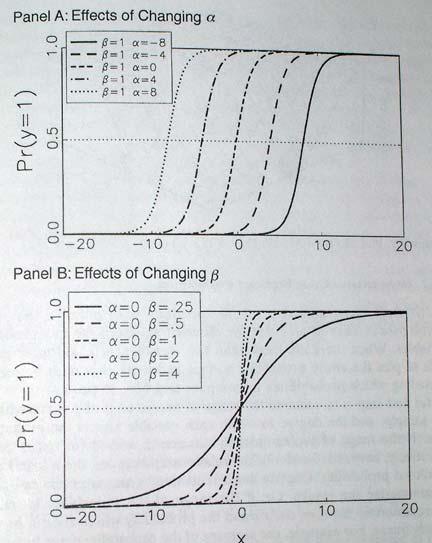
13 . logit marijuana sex age educ childs, robust Logistic regression Number of obs = 845 Wald chi2(4) = Prob > chi2 = Log pseudolikelihood = Pseudo R2 = Robust marijuana Coef. Std. Err. z P> z [95% Conf. Interval] sex age educ childs _cons The two sets of standard errors look the same no violation of assumptions about error distribution. 6. Overdispersion In logistic regression, the expected variance of the dependent variable can be compared to the observed variance, and discrepancies may be considered under- or overdispersion. If there is substantial discrepancy, standard errors will be over-optimistic. The expected variance is ybar*(1 - ybar), where ybar is the mean of the fitted values. This can be compared with the actual variance in observed DV to assess under- or overdispersion. We can see the extent of overdispersion by examining the ratio of D/df (where D is the deviance (-2LL) and df=n-k) -- given that we eliminated other reasons for deviance to be large (e.g., outliers, nonlinearities, other model specification errors like omitted variables). In the fitstat output, we find D(df=840) is The ratio is. di / The ratio is close enough to 1 for us not to worry. If there is overdispersion (which is much more common than underdispersion), we can use adjusted standard errors. Adjusted standard errors will make the confidence intervals wider. Adjusted SE equals SE * sqrt(d/df), where D is the deviance (-2LL) and df=n-k. However, typically overdispersion reflects the fact that we need to respecify the model (i.e. we omitted an important variable), or that our observations are not independent i.e., data over time or clusters of observations. We ll discuss methods to deal with clusters of observation later in the course. Binary Logit Interpretation As logistic regression models (whether binary, ordered, or multinomial) are nonlinear, they pose a challenge for interpretation. The increase in the dependent variable in a linear model is constant for all values of X. Not so for logit models probability increases or decreases per unit change in X is nonconstant, as illustrated in this picture. 13

14 When interpreting logit regression coefficients, we can interpret only the sign and significance of the coefficients cannot interpret the size. The following picture can give you an idea how the shape of the curve varies depending on the size of the coefficient, however. Note that, similarly to OLS regression, the constant determines the position of the curve along the X axis and the coefficient (beta) determines the slope. 14

15 15

16 Next, we ll examine various ways to interpret logistic regression results. 1. Coefficients and Odds Ratios We ll use another model, focusing now on the probability of voting.. codebook vote00 -- vote00 did r vote in 2000 election -- type: numeric (byte) label: vote00 range: [1,4] units: 1 unique values: 4 missing.: 14/2765 tabulation: Freq. Numeric Label voted did not vote ineligible 11 4 refused to answer 14.. gen vote=(vote00==1) if vote00<3 (163 missing values generated). gen married=(marital==1). logit vote age sex born married childs educ Iteration 0: log likelihood = Iteration 1: log likelihood = Iteration 2: log likelihood = Iteration 3: log likelihood = Iteration 4: log likelihood = Logistic regression Number of obs = 2590 LR chi2(6) = Prob > chi2 = Log likelihood = Pseudo R2 = vote Coef. Std. Err. z P> z [95% Conf. Interval] age sex born married childs educ _cons These are regular logit coefficients; so we can interpret the sign and significance but not the size of effects. So we can say that age increases the probability of voting but we can t say by how much that s because a 1 year increase in age will not affect the probability the same way for a 30 year old and for a 40 year old. To be able to interpret effect size, we turn to odds ratios. Note that odds ratios are only appropriate for logistic regression they don t work for probit models. 16

17 Odds are ratios of two probabilities probability of a positive outcome and a probability of a negative outcome (e.g. probability of voting divided by a probability of not voting). But since probabilities vary depending on values of X, such a ratio varies as well. What remains constant is the ratio of such odds e.g. odds of voting for women divided by odds of voting for men will be the same number regardless of the values of other variables. Similarly, the odds ratio for age can be a ratio of the odds of voting for someone who is 31 y.o. to the odds of a 30 y.o. person, or of a 41 y.o. to a 40 y.o. person s odds these will be the same regardless of what age values you pick, as long as they are one year apart. So let s examine the odds ratios.. logit vote age sex born married childs educ, or Iteration 0: log likelihood = Iteration 1: log likelihood = Iteration 2: log likelihood = Iteration 3: log likelihood = Iteration 4: log likelihood = Logistic regression Number of obs = 2590 LR chi2(6) = Prob > chi2 = Log likelihood = Pseudo R2 = vote Odds Ratio Std. Err. z P> z [95% Conf. Interval] age sex born married childs educ Another way to obtain odds ratios would be to use logistic command instead of logit it automatically displays odds ratios instead of coefficients. But yet another, more convenient way is to use listcoef command (that s one of the commands written by Scott Long that we downloaded as a part of spost package):. listcoef logit (N=2590): Factor Change in Odds Odds of: 1 vs vote b z P> z e^b e^bstdx SDofX age sex born married childs educ The advantage of listcoef is that it reports regular coefficients, odds ratios, and standardized odds ratios in one table. Odds ratios are exponentiated logistic regression coefficients. They are sometimes called factor coefficients, because they are multiplicative coefficients. Odds ratios are equal to 1 if there is no effect, smaller than 1 if the effect is negative and larger than 1 if it is positive. So for example, the odds ratio for married indicates that the odds of voting for those who are 17

18 married are 1.63 times higher than for those who are not married. And the odds ratio for education indicates that each additional year of education makes one s odds of voting 1.33 times higher -- or, in other words, increases those odds by 33%. To get percent change directly, we can use percent option:. listcoef, percent logit (N=2590): Percentage Change in Odds Odds of: 1 vs vote b z P> z % %StdX SDofX age sex born married childs educ Beware: if you would like to know what the increase would be per, say, 10 units increase in the independent variable e.g. 10 years of education, you cannot simply multiple the odds ratio by 10! The coefficient, in fact, would be odds ratio to the power of 10. Or alternatively, you could take the regular logit coefficient, multiply it by 10 and then exponentiate it -- e.g. for education:. di exp( *10) di ^ Standardized odds ratios (presented under e^bstdx) are similar to regular odds ratios, but they display the change in the odds of voting per one standard deviation change in the independent variable. The last column in the table generated by listcoef shows what one standard deviation for each variable is. So for age the standardized odds ratio indicates that 17 years of age increase one s odds of voting 2.23 times, or by 123%. Standardized odds ratios, like standardized coefficients in OLS, allow us to compare effect sizes across variables regardless of their measurement units. But, beware of comparing negative and positive effects odds ratios of 1.5 and.5 are not equivalent, even though the first one represents a 50% increase in odds and the second one represents a 50% decrease. This is because odds ratios cannot be below zero (there cannot be a decrease more than 100%), but they do not have an upper bound i.e. can be infinitely high. In order to be able to compare positive and negative effects, we can reverse odds ratios and generate odds ratios for odds of not voting (rather than odds of voting).. listcoef, reverse logit (N=2590): Factor Change in Odds Odds of: 0 vs vote b z P> z e^b e^bstdx SDofX age sex born married childs educ We can see for example that the odds ratio of for born is a negative effect corresponding in size to a positive odds ratio of

19 Listcoef also has a help option that explains what s what in the table:. listcoef, reverse help logit (N=2590): Factor Change in Odds Odds of: 0 vs vote b z P> z e^b e^bstdx SDofX age sex born married childs educ b = raw coefficient z = z-score for test of b=0 P> z = p-value for z-test e^b = exp(b) = factor change in odds for unit increase in X e^bstdx = exp(b*sd of X) = change in odds for SD increase in X SDofX = standard deviation of X 2. Predicted Probabilities In addition to regular coefficients and odds ratios, we also should examine predicted probabilities both for the actual observations in our data and for strategically selected hypothetical cases. Predicted probabilities are always calculated for a specific set of independent variables values. One thing we can calculate is predicted probabilities for the actual data that we have for each case, we take the values of all independent variables and plug it into the equation:. predict prob (option p assumed; Pr(vote)) (26 missing values generated). sum prob if e(sample) Variable Obs Mean Std. Dev. Min Max prob Mean of predicted probabilities represents the average proportion in the sample:. sum vote if e(sample) Variable Obs Mean Std. Dev. Min Max vote These are predicted probabilities for the actual cases in our dataset. It can be useful, however, to calculate predicted probabilities for hypothetical sets of values some interesting combinations that we could compare and contrast.. prvalue logit: Predictions for vote Confidence intervals by delta method 95% Conf. Interval 19

20 Pr(y=1 x): [ , ] Pr(y=0 x): [ , ] age sex born married childs educ x= This calculates a predicted probability for a case with all values set at the mean. So an average person has 72.5% chance of voting. We can also see what these averages are. Clearly, for some variables they don t make sense we don t want to use averages for dummy variables; rather, we d want to specify what values to use. Here are some examples of specifying values:. prvalue, x(age=30 born=1 sex=2 married=0) logit: Predictions for vote Confidence intervals by delta method 95% Conf. Interval Pr(y=1 x): [ , ] Pr(y=0 x): [ , ] age sex born married childs educ x= This is the predicted value for someone who is 30, native born, female, and unmarried (and has average number of children and average education). Note that if you have a set of dummy variables, you should always specify values for each of them in prvalue command. E.g. if we were using 4 marital status dummies, we d have to specify all of them, otherwise, some of them will be assigned their mean values and your calculation will be unrealistic.. xi: qui logit vote age sex born i.marital childs educ. prvalue, x( _Imarital_2=1 _Imarital_3=0 _Imarital_4=0 _Imarital_5=0) logit: Predictions for vote Confidence intervals by delta method 95% Conf. Interval Pr(y=1 x): [ , ] Pr(y=0 x): [ , ] age sex born _Imarital_2 _Imarital_3 _Imarital_4 _Imarital_5 childs educ x= Note: to get the predicted probability for the omitted category, we need to specify all zeros. We can also use prtab to obtain values of predicted probabilities for various combinations of categorical variables we can select one variable at a time or up to four variables in this command but note that we need to specify what values to use for all other variables e.g. in this case, all other variables are set at the mean.. qui logit vote age sex born married childs educ. prtab born married, rest(mean) logit: Predicted probabilities of positive outcome for vote was r born in this married country yes

21 no age sex born married childs educ x= This allows us to see that the effect of one variable depends on the level of the other for native born individuals, marriage increases chances of voting by 9.5%, but for the foreign born, marriage increases these chances by 12.2%. And we can use conditions:. prtab childs born if married ==1 logit: Predicted probabilities of positive outcome for vote was r born in number of this country children yes no none one two three four five six seven eight or more age sex born married childs educ x= But note that the means used in this case are the means for the subgroup specified by these conditions (in this case, for the married). If you want to use the means for the whole sample, you d have to specify them using x option:. prtab childs born if married ==1, x(age= sex= educ= ) logit: Predicted probabilities of positive outcome for vote was r born in number of this country children yes no none one two three four five six seven eight or more age sex born married childs educ x= Note that it only makes sense to create such tables of predicted probabilities for variables that have significant effects otherwise, you ll see no differences. And if you have sets of dummy variables, you are better off using 21

22 prvalue to obtain your predicted values (see above); prtab can be quite confusing for such cases. Further, we can use prgen to generate new variables containing probabilities for certain sets of values. This is useful with continuous variables, as it allows us to see how predicted probability changes across values of one variable (given that the rest of them are set at some specific values). In the following example, we generate predicted values for 7 different ages -- 20, 80, and 5 more points in between. We generate these for four groups defined by education (10, 12, 16, 20). The rest of the variables are set at mean. We ll add labels to the new variables containing predicted probabilities.. for num : prgen age, from (20) to (80) gen(preducx) x(educ=x) rest(mean) n(7) \ lab var preducxp1 "education=x" -> prgen age, from (20) to (80) gen(preduc10) x(educ=10) rest(mean) n(7) logit: Predicted values as age varies from 20 to 80. age sex born married childs educ x= > lab var preduc10p1 `"education=10"' -> prgen age, from (20) to (80) gen(preduc12) x(educ=12) rest(mean) n(7) logit: Predicted values as age varies from 20 to 80. age sex born married childs educ x= > lab var preduc12p1 `"education=12"' -> prgen age, from (20) to (80) gen(preduc16) x(educ=16) rest(mean) n(7) logit: Predicted values as age varies from 20 to 80. age sex born married childs educ x= > lab var preduc16p1 `"education=16"' -> prgen age, from (20) to (80) gen(preduc20) x(educ=20) rest(mean) n(7) logit: Predicted values as age varies from 20 to 80. age sex born married childs educ x= > lab var preduc20p1 `"education=20"' Now we can plot four curves that show how probability of voting changes by age for an average person who has 10, 12, 16, or 10 years of education.. graph twoway connected preduc10p1 preduc12p1 preduc16p1 preduc20p1 preduc20x 22

23 age of respondent education=10 education=16 education=12 education=20 If there are interactions or nonlinearities that required that you entered a variable more than once (e.g. X and X squared), you can use adjust command to do the graphs. This is done in the same manner as we did in OLS, but we need to use pr option to get probabilities rather than linear prediction (xb). This is the best way to examine what interactions mean in logit models, because their value For example we can replicate our previous graph. We run adjust command omitting age and educ:. adjust sex born married childs if e(sample), gen(prob1) pr -- Dependent variable: vote Command: logit Created variable: prob1 Variables left as is: age, educ Covariates set to mean: sex = , born = , married = , childs = All pr Key: pr = Probability. separate prob1, by(educ) storage display value variable name type format label variable label - prob10 float %9.0g prob1, educ == 0 prob11 float %9.0g prob1, educ == 1 prob12 float %9.0g prob1, educ == 2 prob13 float %9.0g prob1, educ == 3 prob14 float %9.0g prob1, educ == 4 prob15 float %9.0g prob1, educ == 5 prob16 float %9.0g prob1, educ == 6 prob17 float %9.0g prob1, educ == 7 prob18 float %9.0g prob1, educ == 8 23

24 prob19 float %9.0g prob1, educ == 9 prob110 float %9.0g prob1, educ == 10 prob111 float %9.0g prob1, educ == 11 prob112 float %9.0g prob1, educ == 12 prob113 float %9.0g prob1, educ == 13 prob114 float %9.0g prob1, educ == 14 prob115 float %9.0g prob1, educ == 15 prob116 float %9.0g prob1, educ == 16 prob117 float %9.0g prob1, educ == 17 prob118 float %9.0g prob1, educ == 18 prob119 float %9.0g prob1, educ == 19 prob120 float %9.0g prob1, educ == 20. line prob110 prob112 prob116 prob120 age, sort age of respondent prob1, educ == 10 prob1, educ == 12 prob1, educ == 16 prob1, educ == Changes in Predicted Probabilities Another way to interpret logistic regression results is using changes in predicted probabilities. These are changes in probability of the outcome as one variable changes, holding all other variables constant at certain values. There are two ways to measure such changes discrete change and marginal effect. A. Discrete change Discrete change is a change in predicted probabilities corresponding to a given change in the independent variable. To obtain these, we calculate two probabilities and then calculate the difference between them. These can be obtained using prvalue command, but it is much easier to do using prchange:. prchange logit: Changes in Probabilities for vote min->max 0->1 -+1/2 -+sd/2 MargEfct age sex born married childs educ Pr(y x) age sex born married childs educ 24

25 x= sd(x)= Here we can see how probability changes when we go from the minimum value of each variable, e.g. education, to its maximum, how it changes when we go from 0 to 1, how it changes per one unit at the mean (that is displayed as -+1/2 because it calculates the differences between mean-1 and mean+1, and then divides it by 2. Then there is the change per one standard deviation, also around the mean. We can also get a clear explanation of what s what using help option:. prchange, help logit: Changes in Probabilities for vote min->max 0->1 -+1/2 -+sd/2 MargEfct age sex born married childs educ Pr(y x) age sex born married childs educ x= sd(x)= Pr(y x): probability of observing each y for specified x values Avg Chg : average of absolute value of the change across categories Min->Max: change in predicted probability as x changes from its minimum to its maximum 0->1: change in predicted probability as x changes from 0 to 1 -+1/2: change in predicted probability as x changes from 1/2 unit below base value to 1/2 unit above -+sd/2: change in predicted probability as x changes from 1/2 standard dev below base to 1/2 standard dev above MargEfct: the partial derivative of the predicted probability/rate with respect to a given independent variable We can also run prchange with fromto option to get starting and ending probabilities in addition to the amount of change:. prchange, fromto logit: Changes in Probabilities for vote from: to: dif: from: to: dif: from: to: dif: from: to: dif: x=min x=max min->max x=0 x=1 0->1 x-1/2 x+1/2 -+1/2 x-1/2sd x+1/2sd -+sd/2 age sex born married childs educ MargEfct age sex born married

26 childs educ Pr(y x) age sex born married childs educ x= sd(x)= We can customize the amount of change in X using delta option, set the value of X to whatever we want, and we can also select uncentered option if we don t want our selected interval to be centered at X but would rather prefer it to start at X. For example, with and without uncentered option:. prchange educ, x(educ=16) delta(4) uncentered logit: Changes in Probabilities for vote (Note: delta = 4) min->max 0->1 +delta +sd MargEfct educ Pr(y x) age sex born married childs educ x= sd(x)= prchange educ, x(educ=16) delta(4) logit: Changes in Probabilities for vote (Note: d = 4) min->max 0->1 -+d/2 -+sd/2 MargEfct educ Pr(y x) age sex born married childs educ x= sd(x)= B. Marginal effects. The last column of prchange output presents marginal effects these are partial derivatives, slopes of probability curve at a certain set of values of independent variables. Marginal effects, of course, vary along X; they are the largest at the value of X that corresponds to P(Y=1 X)=.5 this can be seen in the graph. 26

27 Usually, if marginal effects are presented in journal articles, they are evaluated with all variables held at their means. In case of logistic regression, marginal effect for X can be calculated as P(Y=1 X)*P(Y=0 X)*b; For example, we can replicate the last result, di *0.8475* The following graph compares a marginal change and a discrete change at a specific point: We can also generate marginal effects with standard errors using mfx compute. Computing those standard errors can take a while, however. 27