CrimeStat Version 3.3 Update Notes:

Transcription

1 CrmeStat Verson 3.3 Update Notes: Part 2: Regresson Modelng Ned Levne Domnque Lord Byung-Jung Park Ned Levne & Assocates Zachry Dept. of Korea Transport Insttute Houston, TX Cvl Engneerng Goyang, South Korea Texas A & M Unversty College Staton, TX July 2010

2 Table of Contents Introducton 1 Functonal Relatonshps 1 Normal Lnear Relatonshps 1 Ordnary Least Squares 2 Maxmum Lkelhood Estmaton 3 Assumptons of Normal Lnear Regresson 5 Normal Dstrbuton of Dependent Varable 5 Errors are Independent, Constant, and Normally-dstrbuted 5 Independence of Independent Varables 5 Adequate Model Specfcaton 6 Example of Modelng Burglares by Zones 6 Example Normal Lnear Model 8 Summary Statstcs for the Goodness-of-Ft 8 Statstcs on Indvdual Coeffcents 11 Estmated Error n the Model for Indvdual Coeffcents 13 Volatons of Assumptons for Normal Lnear Regresson 16 Non-constant Summaton 16 Non-lnear Effects 16 Greater Resdual Errors 17 Correctons to Volated Assumptons n Normal Lnear Regresson 17 Elmnatng Unmportant Varables 17 Elmnatng Multcollnearty 18 Transformng the Dependent Varable 19 Example of Transformng the Dependent Varable 19 Count Data Models 21 Posson Regresson 21 Advantages of the Posson Regresson Model 24 Example of Posson Regresson 24 Lkelhood Statstcs 24 Model Error Estmates 25 Over-dsperson Tests 27 Indvdual Coeffcent Statstcs 27 Problems wth the Posson Regresson Model 27 Over-dsperson n the Resdual Errors 27 Posson Regresson wth Lnear Dsperson Correcton 28 Example of Posson Model wth Lnear Dsperson Correcton (NB1) 30 Posson-Gamma (Negatve Bnomal) Regresson 32 Example 1 of Negatve Bnomal Regresson 34 Example 2 of Negatve Bnomal Regresson wth Hghly Skewed Data 34 Advantages of the Negatve Bnomal Model 37 Dsadvantages of the Negatve Bnomal Model 37

3 Table of Contents (contnued) Alternatve Regresson Models 39 Lmtatons of the Maxmum Lkelhood Approach 39 Markov Chan Monte Carlo (MCMC) Smulaton of Regresson Functons 40 Hll Clmbng Analogy 40 Bayesan Probablty 41 Bayesan Inference 42 Markov Chan Sequences 43 MCMC Smulaton 44 Step 1: Specfyng a Model 44 Posson-Gamma Model 44 Posson-Gamma-Condtonal Autoregressve (CAR) Model 45 Spatal Component 45 Step 2: Settng Up a Lkelhood Functon 46 Step 3: Defnng a Jont Posteror Dstrbuton 46 Step 4: Drawng Samples from the Full Condtonal Dstrbuton 47 Step 5: Summarzng the Results from the Sample 49 Why Run an MCMC when MLE s So Easy? 53 Posson-Gamma-CAR Model 54 Negatve Exponental Dstance Decay 55 Restrcted Negatve Exponental Dstance Decay 55 Contguty Functon 55 Example of Posson-Gamma-CAR Analyss of Houston Burglares 56 Spatal Autocorrelaton of the Resduals from the Posson-Gamma-CAR Model 58 Rsk Analyss 62 Issues n MCMC Modelng 66 Startng Values of Each Parameter 66 Example of Defnng Pror Values for Parameters 66 Convergence 68 Montorng Convergence 72 Statstcally Testng Parameters 72 Multcollnearty and Overfttng 72 Multcollnearty 73 Stepwse Varable Entry to Control Multcollnearty 75 Overfttng 76 Condton Number of Matrx 77 Overfttng and Poor Predcton 77 Improvng the Performance of the MCMC Algorthm 78 Scalng of the Data 79 Block Samplng Method for the MCMC 80 Comparson of Block Samplng Method wth Full Dataset 81 Test 1 81

4 Table of Contents (contnued) Test 2 82 Statstcal Testng wth Block Samplng Method 84 The CrmeStat Regresson Module 85 Input Data Set 85 Dependent Varable 85 Independent Varables 87 Type of Dependent Varable 87 Type of Dsperson Estmate 87 Type of Estmaton Method 87 Spatal Autocorrelaton Estmate 87 Type of Test Procedure 87 MCMC Choces 88 Number of Iteratons 88 Burn n Iteratons 88 Block Samplng Threshold 88 Average Block Sze 88 Number of Samples Drawn 88 Calculate Intercept 89 Advanced Optons 89 Intal Parameter Values 89 Rho (ρ) and Tauph (τ ϕ ) 91 Alpha (α) 91 Dagnostc Test for Reasonable Alpha Value 92 Value for 0 Dstances Between Records 93 Output 93 Maxmum Lkelhood (MLE) Model Output 93 MLE Summary Statstcs 93 Informaton About the Model 93 Lkelhood Statstcs 94 Model Error Estmates 94 Over-dsperson Tests 94 MLE Indvdual Coeffcent Statstcs 95 Markov Chan Monte Carlo (MCMC) Model Output 95 MCMC Summary Statstcs 95 Informaton About the Model 95 Lkelhood Statstcs 96 Model Error Estmates 96 Over-dsperson Tests 96 MCMC Indvdual Coeffcent Statstcs 97 Expanded Output (MCMC Only) 98 Output Ph Values (Posson-Gamma-CAR Model Only) 98

5 Table of Contents (contnued) Save Output 99 Save Estmated Coeffcents 99 Dagnostc Tests 99 Mnmum and Maxmum Values for the Varables 99 Skewness Tests 100 Testng for Spatal Autocorrelaton n the Dependent Varable 101 Estmatng the Value of Alpha (α) for the Posson-Gamma-CAR Model 102 Multcollnearty Tests 102 Lkelhood Ratos 102 Regresson II Module 103 References 105 v

6 Introducton 1 The Regresson I and Regresson II modules are a seres of routnes for regresson modelng and predcton. Ths update chapter wll lay out the bascs of regresson modelng and predcton and wll dscuss the CrmeStat Regresson I and II modules. The routnes avalable n the two modules have also been appled to the Trp Generaton model of the Crme Travel Demand module. Users wantng to mplement that model should consult the documentaton n ths update chapter. We start by brefly dscussng the theory and practce of regresson modelng wth examples. Later, we wll dscuss the partcular routnes avalable n CrmeStat. Functonal Relatonshps The am of a regresson model s to estmate a functonal relatonshp between a dependent varable (call t y ) and one or more ndependent varables (call them x1, xk ). In an actual database, these varables have unque names (e.g., ROBBERIES, POPULATION), but we wll use general symbols to descrbe these varables. The functonal relatonshp can be specfed by an equaton (Up. 2.1): y f ( x 1,, x ) (Up. 2.1) K where Y s the dependent varable, x1, xk are the ndependent varables, f ( ) s a functonal relatonshp between the dependent varable and the ndependent varables, and s an error term (essentally, the dfference between the actual value of the dependent varable and that predcted by the relatonshp). Normal Lnear Relatonshps The smplest relatonshp between the dependent varable and the ndependent varables s lnear wth the dependent varable beng normally dstrbuted, y x x K K (Up. 2.2) 1 Ths chapter s a result of the effort of many persons. The maxmum lkelhood routnes were produced by Ian Cahll of Cahll Software n Ottawa, Ontaro as part of hs MLE++ software package. We are grateful to hm for provdng these routnes and for conductng qualty control tests on them. The basc MCMC algorthm n CrmeStat for the Posson-Gamma and Posson-Gamma-CAR models was desgned by Dr. Shaw-Pn Maou of College Staton, TX. We are grateful for Dr. Maou for ths effort. Improvements to the algorthm were made by us, ncludng the block samplng strategy and the calculaton of summary statstcs. The programmer for the routnes was Ms. Hayan Teng of Houston, TX who ensured that they worked. We are also grateful to Dr. Rchard Block of Loyola Unversty n Chcago (IL) for testng the MCMC and MLE routnes.

7 Ths equaton can be wrtten n a smple matrx notaton: y x β where T T x ( 1, x1,, xk ) and β ( 0, 1,, K ). The number one n the frst element of T an ntercept. T denotes that the matrx x s transposed. T T x represents Ths functon says that a unt change n each ndependent varable, x k, for every observaton, s assocated wth a unt change n the dependent varable, y. The coeffcent of each varable, specfes the amount of change n y assocated wth that ndependent varable whle keepng all other ndependent varables n the equaton constant. The frst term, 0, s the ntercept, a constant that s added to all observatons. The error term,, s assumed to be dentcally and ndependently dstrbuted (d) across all observatons, normally dstrbuted wth an expected mean of 0 and a constant standard devaton. If each of the ndependent varables has been standardzed by k, z k xk xk (Up. 2.3) std x ) ( k then the standard devaton of the error term wll be 1.0 and the coeffcents wll be standardzed, b 1, b 2, b 3, and so forth. The equaton s estmated by one of two methods, ordnary least squares (OLS) and maxmum lkelhood estmaton (MLE). Both solutons produce the same results. The OLS method mnmzes the sum of the squares of the resdual errors whle the maxmum lkelhood approach maxmzes a jont probablty densty functon. Ordnary Least Squares Appendx C by Luc Anseln dscusses the method n more depth. Brefly, the ntercept and coeffcents are estmated by choosng a functon that mnmzes the resdual errors by settng N y K 0 k xk xk 0 (Up. 2.4) k 1 1 for k=1 to K ndependent varables or, n matrx notaton: X T ( y Xβ) 0 (Up. 2.5) T T X Xβ X y (Up. 2.6) where T X and y y, y,, ). T ( x1, x2,, x N ) ( 1 2 y N 2

8 3 The soluton to ths system of equatons yelds the famlar matrx expresson for T OLS b K b b ),,, ( 1 0 b y X X X b T T OLS 1 ) ( (Up. 2.7) An estmate for the error varance follows as N K k k k OLS K N x b b y s ) /( - (Up. 2.8) or, n matrx notaton, 1) /( 2 K N s T OLS e e (Up. 2.9) Maxmum Lkelhood Estmaton For the maxmum lkelhood method, the lkelhood of a functon s the jont probablty densty of a seres of observatons (Wkpeda, 2010b; Myers, 1990). Suppose there s a sample of n ndependent observatons ),,, ( 2 1 N x x x that are drawn from an unknown probablty densty dstrbuton but from a known famly of dstrbutons, for example the sngle-parameter exponental famly. Ths s specfed as ) ( θ f where θ s the parameter (or parameters f there are more than one) that defne the unqueness of the famly. The jont densty functon wll be: ) ( ) ( ) ( ),,, ( θ θ θ θ N N x f x f x f x x x f (Up. 2.10) and s called the lkelhood functon: ) ( ),,, ( ),,, ( θ θ θ N N N x f x x x f x x x L (Up. 2.11) where L s the lkelhood and s the product term. Typcally, the lkelhood functon s nterpreted n term of natural logarthms snce the logarthm of a product s a sum of the logarthms of the ndvdual terms. That s, ) ( ln ) ( ln ) ( ln ) ( ln θ θ θ θ n N x f x f x f x f (Up. 2.12) Ths s called the Log lkelhood functon and s wrtten as:

9 N ln L( θ x1, x2,, x ) ln f ( x θ) (Up. 2.13) N 1 For the OLS model, the log lkelhood s: where N s the sample sze and N N N 2 1 T 2 ln L ln(2 ) ln( ) ( y x 2 β) (Up. 2.14) ln L N 1 2 σ s the varance. For the Posson model, the log lkelhood s: y ln( ) ln y! 1 (Up. 2.15) where exp( x T β) s the condtonal mean for zone, and y s the observed number of events for zone. As mentoned, Anseln provdes a more detaled dscusson of these functons n Appendx C. The MLE approach estmates the value of θ that maxmzes the log lkelhood of the data comng from ths famly. Because they are all part of the same mathematcal famly, the maxmum of a jont probablty densty dstrbuton can be easly estmated. The approach s to, frst, defne a probablty functon from ths famly, second, create a jont probablty densty functon for each of the observatons (the Lkelhood functon); thrd, convert the lkelhood functon to a log lkelhood; and, fourth, estmate the value of parameters that maxmze the jont probablty through an approxmaton method (e.g., Newton-Raphson or Fsher scores). Because the functon s regular and known, the soluton s relatvely easy. Anseln dscusses the approach n detal n Appendx C of the CrmeStat manual. More detal can be found n Hlbe (2008). In CrmeStat, we use the MLE method. Because the OLS method s the most commonly used, a normal lnear model s sometmes called an Ordnary Least Squares (OLS) regresson. If the equaton s correctly specfed (.e., all relevant varables are ncluded), the error term,, wll be normally 2 dstrbuted wth a mean of 0 and a constant varance, σ. The OLS normal estmate s sometmes known as a Best Lnear Unbased Estmate (BLUE) snce t mnmzes the sum of squares of the resduals errors (the dfference between the observed and predcted values of y ). In other words, the overall ft of the normal model estmated through OLS or maxmum lkelhoods wll produce the best overall ft for a lnear model. However, keep n mnd that because a normal functon has the best overall ft does not mean that t fts any partcular secton of the dependent varable better. In partcular, for count data, the normal model often does a poor job of modelng the observatons wth the greatest number of events. We wll demonstrate ths wth an example below. 4

10 Assumptons of Normal Lnear Regresson The normal lnear model has some assumptons. When these assumptons are volated, problems can emerge n the model, sometmes easly correctable and other tmes ntroducng substantal bas. Normal Dstrbuton of Dependent Varable Frst, the normal lnear model assumes that the dependent varable s normally dstrbuted. If the dependent varable s not exactly normally dstrbuted, t has to have ts peak somewhere n the mddle of the data range and be somewhat symmetrcal (e.g., a quartc dstrbuton; see chapter 8 n the CrmeStat manual). For some varables, ths assumpton s reasonable (e.g., wth heght or weght of ndvduals). However, for most varables that crme researchers work wth (e.g., number of robberes, number of homcdes, journey-to-crme dstances), ths assumpton s usually volated. Most varables that are counts (.e., number of dscrete events) are hghly skewed. Consequently, when t comes to counts and other extremely skewed varables, the normal (OLS) model may produce dstorted results. Errors are Independent, Constant, and Normally-dstrbuted Second, the errors n the model, the ε n equaton Up. 2.2, must be ndependent of each other, constant, and normally dstrbuted. Ths fts the d assumpton mentoned above. Independence means that the estmaton error for any one observaton cannot be related to the error for any other observaton. Constancy means that the amount of error should be more or less the same for every observaton; there wll be natural varablty n the errors, but ths varablty should be dstrbuted normally wth the mean error beng the expected value. Unfortunately, for most of the varables that crme researchers and analysts work wth, ths assumpton s usually volated. Wth count varables, the errors ncrease wth the count and are much hgher for observatons wth large counts than for observaton wth few counts. Thus, the assumpton of constancy s volated. In other words, the varance of the error term s a functon of the count. The shape of the error dstrbuton s also sometmes not normal ether but may be more skewed. Also, f there s spatal autocorrelaton among the error terms (whch would be expected n a spatal dstrbuton), then the error term may be qute rregular n shape; n ths latter case, the assumpton of ndependent observatons would also be volated. Independence of Independent Varables Thrd, an assumpton of the normal model (and any model, for that matter) s that the ndependent varables are truly ndependent. In theory, there should be zero correlaton between any of the ndependent varables. In practce, however, many varables are related, sometmes qute hghly. Ths condton, whch s called multcollnearty, can sometmes produce dstorted coeffcents and overall model effects. The hgher the degree of multcollnearty among the ndependent varables, the greater the dstorton n the coeffcents. Ths problem affects all types of models, not just the normal, and t s 5

11 mportant to mnmze the effects. We wll dscuss dagnostc methods for dentfyng multcollnearty later n the chapter. Adequate Model Specfcaton Fourth, the normal model assumes that the ndependent varables have been correctly specfed. That s, the ndependent varables are the correct ones to nclude n the equaton and that they have been measured adequately. By correct ones, we mean that the ndependent varable chosen should be a true predctor of the dependent varable, not an extraneous one. Wth any model, the more ndependent varables that are added to the equaton, n general the greater wll be the overall ft. Ths wll be true even f the ndependent varables are hghly correlated wth ndependent varables already n the equaton or are mostly rrelevant (but may be slghtly correlated due to samplng error). When too many varables are added to an equaton, strange effects can occur. Overfttng of a model s a serous problem that must be serously evaluated. Includng too many varables wll also artfcally ncrease the model s varance (Myers, 1990). Conversely, a correct specfcaton mples that all the mportant varables have been ncluded and that none have been left out. When mportance varables are not ncluded, ths s called underfttng a model. Also, not ncludng mportant varables lead to a based model (known as the omtted varables bas). A large bas means that the model s unrelable for predcton (Myers, 1990). Also, the left out varables can be shown to have rregular effects on the error terms. For example, f there s spatal autocorrelaton n the dependent varable (whch there usually s), then the error terms wll be correlated. Wthout modelng the spatal autocorrelaton (ether through a proxy varable that captures much of ts effect or through a parameter adjustment), the error can be based and even the coeffcents can be based. In other words, adequate specfcaton nvolves choosng the correct number of ndependent varables that are approprate, nether overfttng nor underfttng of the model. Also, t s assumed that the varables have been correctly measured and that the amount of measurement error s very small. Unfortunately, we often do not know whether a model s correctly specfed or not, nor whether the varables have been properly measured. Consequently, there are a number of dagnostcs tests that can be brought to bear to reveal whether the specfcaton s adequate. For overfttng, there are tolerance statstcs and adjusted summary values. For underfttng, we analyze the error dstrbuton to see f there s a pattern that mght ndcate lurkng varables that are not ncluded n the model. In other words, examnng volatons of the assumptons of a model s an mportant task n assessng whether there are too many varables ncluded or whether there are varables that should be ncluded but are not, or whether the specfcaton of the model s correct or not. Ths s an mportant task n regresson modelng. Example of Modelng Burglares by Zones For many problems, normal regresson s an approprate tool. However, for many others, t s not. Let us llustrate ths pont. A note of cauton s warranted here. Ths example s used to llustrate the applcaton of the normal model n CrmeStat and, as dscussed further below, the normal model wth a normal error dstrbuton s not approprate for ths knd of dataset. For example, fgure Up. 2.1 show 6

12 Fgure Up. 2.1:

13 the number of resdental burglares that occurred n 2006 wthn 1,179 Traffc Analyss Zones (TAZ) nsde the Cty of Houston. The data on burglares came from the Houston Polce Department. The burglares were then allocated to the 1,179 traffc analyss zones wthn the Cty of Houston. As can be seen, there s a large concentraton of resdental burglares n southwest Houston wth small concentratons n southeast Houston and n parts of north Houston. The dstrbuton of burglares by zones s qute skewed. Fgure Up. 2.2 show a graph of the number of burglares per zone. Of the 1,179 traffc analyss zones, 250 had no burglares occur wthn them n On the other hand, one zone had 284 burglares occur wthn t. The graph show the number of burglares up to 59; there were 107 zones wth 60 or more burglares that occurred n them. About 58% of the burglares occurred n 10% of the zones. In general, a small percentage of the zones had the majorty of the burglares, a result that s very typcal of crme counts. Example Normal Lnear Model We can set up a normal lnear model to try to predct the number of burglares that occurred n each zone n We obtaned estmates of populaton, employment and ncome from the transportaton modelng group wthn the Houston-Galveston Area Councl, the Metropoltan Plannng Organzaton for the area (H-GAC, 2010). Specfcally, the model relates the number of 2006 burglares to the number of households, number of jobs (employment), and medan ncome of each zone. The estmates for the number of households and jobs were for 2006 whle the medan ncome was that measured by the 2000 census. Table Up. 2.1 present the results of the normal (OLS) model. Summary Statstcs for the Goodness-of-Ft The table presents two types of results. Frst, there s summary nformaton. Informaton on the sze of the sample (n ths case, 1,179) and the degrees of freedom (the sample sze less one for each parameter estmated ncludng the ntercept and one for the mean of the dependent varable); n the example, there are 1,174 degrees of freedom (1,179 1 for the ntercept, 1 for HOUSEHOLDS, 1 for JOBS, 1 for MEDIAN HOUSEHOLD INCOME, and 1 for the mean of the dependent varable, 2006 BURGLARIES). The F-test presents an Analyss of Varance test of the rato of the mean square error (MSE) of the model compared to the total mean square error (Kanj, 1994, 131; Abraham & Ledolter, 2006, 41-51). Next, there s the R-square (or R 2 ) statstc, whch s the most common type of overall ft test. Ths s the percent of the total varance of the dependent varable accounted for by the model. More formally, t s defned as: R 2 ( y ˆ y ) 1 2 ( y y) 2 (Up. 2.16) 8

14 Fgure Up. 2.2: Houston Burglares n 2006: Number of Burglares Per Zone 200 Numbe er of zones Number of burglares per zone

15 Table Up. 2.1: Predctng Burglares n the Cty of Houston: 2006 Ordnary Least Squares: Full Model (N= 1,179 Traffc Analyss Zones) DepVar: 2006 BURGLARIES N: 1,179 Df: 1,174 Type of regresson model: Ordnary Least Squares F-test of model: p.0001 R-square: 0.48 Adjusted r-square: 0.48 Mean absolute devaton: st (hghest) quartle: nd quartle: rd quartle: th (lowest) quartle: 8.8 Mean squared predctve error: st (hghest) quartle: 1, nd quartle: rd quartle: th (lowest) quartle: Predctor DF Coeffcent Stand Error Tolerance t-value p INTERCEPT HOUSEHOLDS JOBS n.s. MEDIAN HOUSEHOLD INCOME where y s the observed number of events for a zone,, ŷ s the predcted number of events gven a set of K ndependent varables, and Mean y s the mean number of events across zones. The R-square value s a number from 0 to 1; 0 ndcates no predctablty whle 1 ndcates perfect predctablty. For a normal (OLS) model, R-square s a very consstent estmate. It ncreases n a lnear manner wth predctablty and s a good ndcator of how effectve a model has ft the data. As wth all dagnostc statstcs, the value of the R-square ncreases wth more ndependent varables. Consequently, an R-square adjusted for degrees of freedom s also calculated - the adjusted r-square n the table. Ths s ( y 2 ˆ ) /( 1) 2 y N K Ra 1 (Up. 2.17) 2 ( y y) /( N 1) 10

16 where N s the sample sze and K s the number of ndependent varables. The R 2 value s sometmes called the coeffcent of determnaton. It s an ndcator of the extent to whch the ndependent varables n the model predct (or explan) the dependent varable. One nterpretaton of the R 2 s the percent of the varance of Y accounted for by the varance of the ndependent varables (plus the ntercept and any other constrants added to the model). The unexplaned varance s 1 - R 2 or the extent to whch the model does not explan the varance of the dependent varable. For a normal lnear model, the R 2 s relatvely straghtforward. In the example, both the F-test s hghly sgnfcant and the R 2 s substantal (48% of the varance of the dependent varable s explaned by the ndependent varables). However, for non-lnear models, t s not at all an ntutve measure and has been shown to be unrelable (Maou, 1996). The fnal two summary measures are Mean Squared Predctve Error (MSPE), whch s the average of the squared resdual errors, and the Mean Absolute Devaton (MAD), whch s the average of the absolute value of the resdual errors (Oh, Lyon, Washngton, Persaud, & Bared, 2003). The lower the values of these measures, the better the model fts the data. These measures are also calculated for specfc quartles. The 1 st quartle represents the error assocated wth the 25% of the observatons that have the hghest values of the dependent varable whle the 4 th quartle represents the error assocated wth the 25% of the observatons wth the lowest value of the dependent varable. These percentles are useful for examnng how well a model fts the data and whether the ft s better for any partcular secton of the dependent varable. In the example, the ft s better for the low end of the dstrbuton (the zones wth zero or few burglares) and less good for the hgher end. We wll use these values n comparng the normal model to other models. It s mportant to pont out that the summary measures are more useful when several models wth a dfferent number of varables are compared wth each other than for evaluatng a sngle model. Statstcs on Indvdual Coeffcents The second type of nformaton presented s about each of the coeffcents. The table lsts the ndependent varable plus the ntercept. For each coeffcent, the degrees of freedom assocated are presented (one per varable) plus the estmated lnear coeffcent. For each coeffcent, there s an estmated standard error, a t-test of the coeffcent (the coeffcent dvded by the standard error), and the approxmate two-taled probablty level assocated wth the t-test (essentally, an estmate of the probablty that the null hypothess of zero coeffcent s correct). Usually, f the probablty level s smaller than 5% (.05), then we reject the null hypothess of a zero coeffcent though frequently 1% (.01) or even 0.1% (0.001) have been used to reduce the lkelhood that a false alternatve hypothess has been selected (called a Type I error). The last parameter ncluded n the table s the tolerance of the coeffcent. Ths s a measure of multcollnearty (or one type of overfttng). Bascally, t s the extent to whch each ndependent varable correlates wth the other dependent varables n the equaton. The tradtonal tolerance test s a 11

17 normal model relatng each ndependent varable to the other ndependent varables (StatSoft, 2010; Berk, 1977). It s defned as: Tol 2 1 R j (Up. 2.18) 2 where R j s the R-square assocated wth the predcton of one ndependent varable wth the remanng ndependent varables n the model. In other words, the tolerance of each ndependent varable s the unexplaned varance of a model that relates the varable to the other ndependent varables. If an ndependent varable s hghly related to (correlated wth) the other ndependent varables n the equaton, then t wll have a low tolerance. Conversely, f an ndependent varable s ndependent of the other ndependent varables n the equaton, then t wll have a hgh tolerance. In theory, the hgher the tolerance, the better snce each ndependent varable should be unrelated to the other ndependent varables. In practce, there s always some degree of overlap between the ndependent varables so that a tolerance of 1.0 s rarely, f ever, acheved. However, f the tolerance s low (e.g., 0.70 or below), ths suggests that there s too much overlap n the ndependent varables and that the nterpretaton wll be unclear. Later n the chapter, we wll dscuss multcollnearty and the general problem of overfttng n more detal. Lookng specfcally at the model n Table Up. 2.1, we see that the number of burglares s postvely assocated wth the ntercept and the number of households and negatvely assocated wth the medan household ncome. The relatonshp to the number of jobs s also negatve, but not sgnfcant. Essentally, zones wth larger numbers of households but lower household ncomes are assocated wth more resdental burglares. Because the model s lnear, each of the coeffcents contrbutes to the predcton n an addtve manner. The ntercept s and ndcates that, on average, each zone had burglares. For every household n the zone, there was a contrbuton of burglares. For every job n the zone, there was a contrbuton of burglares. For every dollar ncrease n medan household ncome, there s a decrease of burglares. Thus, to predct the number of burglares wth the full model n any one zone,, we would take the ntercept 12.93, and add n each of these components: ( BURGLARIES) ( HOUSEHOLDS) ( MEDIAN HOUSEHOLD INCOME) ( JOBS) (Up. 2.19) To llustrate, TAZ 833 had 1762 households n 2006, 2,698 jobs also n 2006, and had a medan household ncome of $27,500 n The model s predcton for the number of burglares n TAZ 833 s: Number of burglares (TAZ833) = * *2, *27,500 = 52.0 The actual number of burglares that occurred n TAZ 833 was

18 Estmated Error n the Model for Indvdual Coeffcents In CrmeStat, and n most statstcal packages, there s addtonal nformaton that can be output as a fle. There s the predcted value for each observaton. Essentally, ths s the lnear predcton from the model. There s also the resdual error, whch s the dfference between the actual (observed) value for each observaton,, and that predcted by the model. It s defned as: Resdual error = Observed Value - Predcted value (Up. 2.20) Table Up. 2.2 gve predcted values and resdual errors for fve of the observatons from the Houston burglary data set. Table Up. 2.2: Predcted Values and Resdual Error for Houston Burglares: 2006 (5 Traffc Analyss Zones) Zone (TAZ) Actual value Predcted value Resdual error Analyss of the resdual errors s one of the best tools for dagnosng problems wth the model. A plot of the resdual errors aganst the predcted values ndcates whether the predcton s consstent across all values of the dependent varable and whether the underlyng assumptons of the normal model are vald (see below). Fgure Up. 2.3 show a graph of the resdual errors of the full model aganst the predcted values for the model estmated n table 1. As can be seen, the model fts qute well for zones wth few burglares, up to about 12 burglares per zone. However, for the zones wth many predcted burglares (the ones that we are most lkely nterested n), the model does qute poorly. Frst, the errors ncrease the greater than number of predcted burglares. Sometmes the errors are postve, meanng that the actual number of burglares s much hgher than predcted and sometmes the errors are negatve, meanng that we are predctng more burglares than actually occurred. More mportantly, the resdual errors ndcate that the model has volated one of the basc assumptons of the normal model, namely that the errors are ndependent, constant, and dentcallydstrbuted. It s clear that they are not. Because there are errors n predctng the zones wth the hghest number of burglares and because the zones wth the hghest number of burglares were somewhat concentrated, there are spatal dstortons from the predcton. Fgure Up. 2.4 show a map of the resdual errors of the normal model. As can be seen by comparng ths map wth the map of burglares (fgure Up. 2.1), typcally the zones 13

19 Fgure Up. 2.3:

20 Fgure Up. 2.4:

21 wth the hghest number of burglares (mostly n southwest Houston) were under-estmated by the normal model (shown n red) whereas some zones wth few burglares ended up beng over-estmated by the normal model (e.g., n far southeast Houston). In other words, the normal lnear model s not necessarly good for predctng Houston burglares. It tends to underestmate zones wth a large number of burglares but overestmates zones wth few. Volatons of Assumptons for Normal Lnear Regresson There are several defcences wth the normal (OLS) model. Frst, normal models are not good at descrbng skewed dependent varables, as we have shown. Snce crme dstrbutons are usually skewed, ths s a serous defcency for multvarate crme analyss. Second, a normal model can have negatve predctons. Wth a count varable, such as the number of burglares commtted n a zone, the mnmum number s zero. That s, the count varable s always postve, beng bounded by 0 on the lower lmt and some large number on the upper lmt. The normal model, on the other hand, can produce negatve predcted values snce t s addtve n the ndependent varables. Ths clearly s llogcal and s a major problem wth data that are hghly skewed. If most records have values close to zero, t s very possble for a normal model to predct a negatve value. Non-consstent Summaton A thrd problem wth the normal model s that the sum of the observed values does not necessarly equal the sum of the predcted values. Snce the estmates of the ntercept and coeffcents are obtaned by mnmzng the sum of the squared resdual errors (or maxmzng the jont probablty dstrbuton, whch leads to the same result), there s no balancng mechansm to requre that they add up to the same as the nput values. In calbratng the model, adjustments can be made to the ntercept term to force the sum of the predcted values to be equal to the sum of the nput values. But n applyng that ntercept and coeffcents to another data set, there s no guarantee that the consstency of summaton wll hold. In other words, the normal method cannot guarantee a consstent set of predcted values. Non-lnear Effects A fourth problem wth the normal model s that t assumes the ndependent varables are normal n ther effect. If the dependent varable was normal or relatvely balanced, then a normal model would be approprate. But, when the dependent varable s hghly skewed, as s seen wth these data, typcally the addtve effects of each component cannot usually account for the non-lnearty. Independent varables have to be transformed to account for the non-lnearty and the result s often a complex equaton wth non-ntutve relatonshps. 2 It s far better to use a non-lnear model for a hghly skewed dependent varable. 2 For example, to account for the skewed dependent varable, one or more of the ndependent varables have to be transformed wth a non-lnear operator (e.g., log or exponental term). When more than one ndependent varable s non-lnear n an equaton, the model s no longer easly understood. It may end up makng reasonable predctons for the dependent varable, but t s not ntutve nor easly explaned to non-specalsts. 16

22 Greater Resdual Errors The fnal problem wth a normal model and a skewed dependent varable s that the model tends to over- or under-predct the correct values, but rarely comes up wth the correct estmate. As we saw wth the example above, typcally a normal equaton produces non-constant resdual errors wth skewed data. In theory, errors n predcton should be uncorrelated wth the predcted value of the dependent varable. Volaton of ths condton s called heteroscedastcty because t ndcates that the resdual varance s not constant. The most common type s an ncrease n the resdual errors wth hgher values of the predcted dependent varable. That s, the resdual errors are greater at the hgher values of the predcted dependent varable than at lower values (Draper and Smth, 1981, 147). A hghly skewed dstrbuton tends to encourage ths. Because the least squares procedure mnmzes the sum of the squared resduals, the regresson lne balances the lower resduals wth the hgher resduals. The result s a regresson lne that nether fts the low values nor the hgh values. For example, motor vehcle crashes tend to concentrate at a few locatons (crash hot spots). In estmatng the relatonshp between traffc volume and crashes, the hot spots tend to unduly nfluence the regresson lne. The result s a lne that nether fts the number of expected crashes at most locatons (whch s low) nor the number of expected crashes at the hot spot locatons (whch are hgh). Correctons to Volated Assumptons n Normal Lnear Regresson Some of the volatons n the assumptons of an OLS normal model can be corrected. Elmnatng Unmportant Varables One good way to mprove a normal model s to elmnate varables that are not mportant. Includng varables n the equaton that do not contrbute very much adds nose (varablty) to the estmate. In the above example, the varable, JOBS, was not statstcally sgnfcant and, hence, dd not contrbute any real effect to the fnal predcton. Ths s an example of overfttng a model. Whether we use the crtera of statstcal sgnfcance to elmnate non-essental varables or smply drop those wth a very small effect s less mportant than the need to reduce the model to only those varables that truly predct the dependent varable. We wll dscuss the pros and cons of droppng varables a lttle later n the chapter, but for now we argue that a good model - one that wll be good not just for descrpton but for predcton, s usually a smple model wth only the strongest varables ncluded. To llustrate, we reduce the burglary model further by droppng the non-sgnfcant varable (JOBS). Table Up. 2.3 show the results. Comparng the results wth Table Up. 2.1, we can see that the overall ft of the model s actually slghtly better (an F-value of compared to 357.2). The R 2 values are the same whle the mean squared predctve error s slghtly worse whle the mean absolute devaton s slghtly better. The coeffcents for the two common ndependent varables are almost dentcal whle that for the ntercept s slghtly less (whch s good snce t contrbutes less to the overall result). 17

23 Table Up. 2.3: Predctng Burglares n the Cty of Houston: 2006 Ordnary Least Squares: Reduced Model (N= 1,179 Traffc Analyss Zones) DepVar: 2006 BURGLARIES N: 1,179 Df: 1,175 Type of regresson model: Ordnary Least Squares F-test of model: p.0001 R-square: 0.48 Adjusted r-square: 0.48 Mean absolute devaton: st (hghest) quartle: nd quartle: rd quartle: th (lowest) quartle: 8.8 Mean squared predctve error: st (hghest) quartle: nd quartle: rd quartle: th (lowest) quartle: Predctor DF Coeffcent Stand Error Tolerance t-value p INTERCEPT HOUSEHOLDS MEDIAN HOUSEHOLD INCOME In other words, droppng the non-sgnfcant varable has led to a slghtly better ft. One wll usually fnd that droppng non-sgnfcant or unmportant varables makes models more stable wthout much loss of predctablty, and conceptually they become smpler to understand. Elmnatng Multcollnearty Another way to mprove the stablty of a normal model s to elmnate varables that are substantally correlated wth other ndependent varables n the equaton. Ths s the multcollnearty problem that we dscussed above. Even f a varable s statstcally sgnfcant n a model, f t s also correlated wth one or more of the other varables n the equaton, then t s capturng some of the varance assocated wth those other varables. The results are ambguty n the nterpretaton of the coeffcents as well as error n tryng to use the model for predcton. Multcollnearty means that essentally there s overlap n the ndependent varables; they are measurng the same thng. It s better to drop a multcollnear varable even f t results n a loss n ft snce t wll usually result n a smpler and less varable model. 18

24 For the Houston burglary example, the two remanng ndependent varables n Table Up. 2.3 are relatvely ndependent; ther tolerances are respectvely, whch ponts to lttle overlap n the varance that they account for n the dependent varable. Therefore, we wll keep these varables. However, later n the chapter n the dscusson of the negatve bnomal model, we wll present an example of how multcollnearty can lead to ambguous coeffcents. Transformng the Dependent Varable It may be possble to correct the normal model by transformng the dependent varable (n another program snce CrmeStat does not currently do ths). Typcally, wth a skewed dependent varable and one that has a large range n values, a natural log transformaton of the dependent varable can be used to reduce the amount of skewness. That s, one takes: ln y log ( y ) (Up. 2.21) e where e s the base of the natural logarthm (2.718 ) and regresses the transformed dependent varable aganst the lnear predctors, ln y x x (Up. 2.22) K K Ths s equvalent to the equaton y e x x K K (Up. 2.23) wth, agan, e beng the base of the natural logarthm. In dong ths, t s assumed that the log transformed dependent varable s consstent wth the assumptons of the normal model, namely that t s normally dstrbuted wth an ndependent and constant error term, ε, that s also normally dstrbuted. One must be careful about transformng values that are zero snce the natural log of 0 s unsolvable. Usually researchers wll set the value of the log-transformed dependent varable to 0 or the values of the dependent varable to a very small number (e.g., 0.001) for cases where the raw dependent varable actually has a value of 0. Whle ths seems lke a reasonable soluton to the problem, t can lead to strange results. In the burglary data, for example, there were 250 zones (out of 1,179 or 21%) that had zero burglares! Example of Transformng Dependent Varable To llustrate, we transformed the dependent varable n the above example number of 2006 burglares per TAZ, by takng the natural logarthm of t. All zones wth zero burglares were automatcally gven the value of 0 for the transformed varable. The transformed varable was then 19

25 regressed aganst the two ndependent varables n the reduced form model (from Table Up. 2.3 above). Table Up. 2.4 present the results: Table Up. 2.4: Predctng Burglares n the Cty of Houston: 2006 Log Transformed Dependent Varable (N= 1,179 Traffc Analyss Zones) DepVar: Natural log of 2006 BURGLARIES N: 1,179 Df: 1,175 Type of regresson model: Ordnary Least Squares F-test of model: p.0001 R-square: 0.42 Adjusted r-square: 0.42 Mean absolute devaton: st (hghest) quartle: nd quartle: rd quartle: th (lowest) quartle: 4.6 Mean squared predctve error: 30, st (hghest) quartle: 118, nd quartle: rd quartle: th (lowest) quartle: Predctor DF Coeffcent Stand Error Tolerance t-value p INTERCEPT HOUSEHOLDS MEDIAN HOUSEHOLD INCOME The coeffcents are smlar n sgn. The R 2 value s smaller than the untransformed model (0.42 compared to 0.48). However, the mean squared predctve error s now much hgher than the orgnal raw values (30, compared to ) and the mean absolute devaton s also much hgher (30.73 compared to 13.50). 3 3 The errors were calculated by, frst, transformng the dependent varable by takng ts natural log; second, the natural log was then regressed aganst the ndependent varables; thrd, the predcted values were then calculated; and, fourth, the predcted values were then converted back nto raw scores by takng them as the exponents of e, the base of the natural logarthm. The resdual errors were calculated from the re-transformed predcted values. 20

26 In other words, transformng the dependent to a natural log has not mproved the overall normal model and, n fact, worsened the predctablty. The hgh degree of skewness n the dependent varable was not elmnated by transformng t. Another type of transformaton that s sometmes used s to convert the ndependent varables and, occasonally, the dependent varable nto Z-scores. The Z-score of a varable s defned as: z k xk xk (Up. 2.24) std x ) ( k But all ths wll do s to standardze the scale of the varable as standard devatons around an expected value of zero, but not alter the shape. If the dependent varable s skewed, takng the Z-score of t wll not alter ts skewness. Essentally, skewness s a fundamental property of a dstrbuton and the normal model s poorly suted for modelng t. Count Data Models In short, a normal lnear model s nadequate for descrbng skewed dstrbutons, partcularly counts. Gven that crme analyss usually nvolves the analyss of counts, ths s a serous defcency. Posson Regresson Consequently, we turn to count data models, n partcular the Posson famly of models. Ths famly s part of the generalzed lnear models (GLMs), n whch the OLS normal model descrbed above s a specal case (McCullagh & Nelder, 1989). Posson regresson s a modelng method that overcomes some of the problems of tradtonal normal regresson n whch the errors are assumed to be normally dstrbuted (Cameron & Trved, 1998). In the model, the number of events s modeled as a Posson random varable wth a probablty of occurrence beng: y e Prob( y ) (Up. 2.25) y! where y s the count for one group or class,, s the mean count over all groups, and e s the base of the natural logarthm. The dstrbuton has a sngle parameter,, whch s both the mean and the varance of the functon. The law of rare events assumes that the total number of events wll approxmate a Posson dstrbuton f an event occurs n any of a large number of trals but the probablty of occurrence n any gven tral s small and assumed to be constant (Cameron & Trved, 1998). Thus, the Posson dstrbuton s very approprate for the analyss of rare events such as crme ncdents (or motor vehcle crashes or uncommon dseases or any other rare event). The Posson model s not partcularly good f the probablty of an event s more balanced; for that, the normal dstrbuton s a better model as the 21

27 samplng dstrbuton wll approxmate normalty wth ncreasng sample sze. Fgure Up.2.5 llustrates the Posson dstrbuton for dfferent expected means (repeated from chapter 13). The mean can, n turn, be modeled as a functon of some other varables (the ndependent T varables). Gven a set of observatons on one or more ndependent varables, x 1, x,, x ), the condtonal mean of y can be specfed as an exponental functon of the x s: ( 1 K T x β E( y x ) e (Up. 2.26) where s an observaton, T ( 0, 1,, K ) T x s a set of ndependent varables ncludng an ntercept, β are a set of coeffcents, and e s the base of the natural logarthm. Equaton Up s sometmes wrtten as K T ln( ) x β x (Up. 2.27) 0 k1 k k where each ndependent varable, k, s multpled by a coeffcent, k, and s added to a constant, 0. In expressng the equaton n ths form, we have transformed t usng a lnk functon, the lnk beng the loglnear relatonshp. As dscussed above, the Posson model s part of the GLM framework n whch the functonal relatonshp s expressed as a lnear combnaton of predctve varables. Ths type of model s sometmes known as a loglnear model, especally f the ndependent varables are categores, rather than contnuous (real) varables. However, we wll refer to t as a Posson model. In more famlar notaton, ths s ln( ) x x x (Up. 2.28) K K That s, the natural log of the mean s a functon of K ndependent varables and an ntercept. The data are assumed to reflect the Posson model. Also, n the Posson model, the varance equals the mean. Therefore, t s expected that the resdual errors should ncrease wth the condtonal mean. That s, there s nherent heteroscedastcty n a Posson model (Cameron & Trved, 1998). Ths s very dfferent than a normal model where the resdual errors are expected to be constant. The model s estmated usng a maxmum lkelhood procedure, typcally the Newton-Raphson method or, occasonally, usng Fsher scores (Wkpeda, 2010a; Cameron & Trved, 1998). In Appendx C, Anseln presents a more formal treatment of both the normal and Posson regresson models ncludng the methods by whch they are estmated. 22

28 Fgure Up. 2.5:

29 Advantages of the Posson Regresson Model The Posson model overcomes some of the problems of the normal model. Frst, the Posson model has a mnmum value of 0. It wll not predct negatve values. Ths makes t deal for a dstrbuton n whch the mean or the most typcal value s close to 0. Second, the Posson s a fundamentally skewed model; that s, t s data characterzed wth a long rght tal. Agan, ths model s approprate for counts of rare events, such as crme ncdents. Thrd, because the Posson model s estmated by a maxmum lkelhood method, the estmates are adapted to the actual data. In practce, ths means that the sum of the predcted values s vrtually dentcal to the sum of the nput values, wth the excepton of a very slght roundng off error. Fourth, compared to the normal model, the Posson model generally gves a better estmate of the counts for each record. The problem of over- or underestmatng the number of ncdents for most zones wth the normal model s usually lessened wth the Posson. When the resdual errors are calculated, generally the Posson has a lower total error than the normal model. In short, the Posson model has some desrable statstcal propertes that make t very useful for predctng crme ncdents. Example of Posson Regresson Usng the same Houston burglary database, we estmate a Posson model of the two ndependent predctors of burglares (Table Up. 2.5). Lkelhood Statstcs The summary statstcs are qute dfferent from the normal model. In the CrmeStat mplementaton, there are fve separate statstcs about the lkelhood, representng a jont probablty functon that s maxmzed. Frst, there s the log lkelhood (L). The lkelhood functon s the jont (product) densty of all the observatons gven values for the coeffcents and the error varance. The log lkelhood s the log of ths product or the sum of the ndvdual denstes. Because the functon t maxmzes s a probablty and s always less than 1.0, the log lkelhood s always negatve wth a Posson model. Second, the Akake Informaton Crteron (AIC) adjusts the log lkelhood for degrees of freedom snce addng more varables wll always ncrease the log lkelhood. It s defned as: AIC = -2L + 2(K+1) (Up. 2.29) where L s the log lkelhood and K s the number of ndependent varables. Thrd, another measure whch s very smlar s the Bayes Informaton Crteron (or Schwartz Crteron), whch s defned as: BIC/SC = -2L+[(K+1)ln(N)] (Up. 2.30) 24

30 These two measures penalze the number of parameters added n the model, and reverse the sgn of the log lkelhood (L) so that the statstcs are more ntutve. The model wth the lowest AIC or BIC/SC values are best. Fourth, a decson about whether the Posson model s approprate can be based on the statstc called the devance whch s defned as: N y Dev 2( L F LM ) 2 y ln y ˆ 1 ˆ (Up. 2.31) where L F s the log lkelhood that would be acheved f the model gave a perfect ft and LM s the loglkelhood of the model under consderaton. If the latter model s correct, the devance (Dev) s 2 approxmately dstrbuted wth degrees of freedom equal to N ( K 1). A value of the devance greatly n excess of N ( K 1) suggests that the model s overdspersed due to mssng varables or non-posson form. Ffth, there s the Pearson ch-square statstc whch s defned by N 2 2 ( y ˆ Pearson ) (Up. 2.32) ˆ 1 and s approxmately ch-square dstrbuted wth mean N ( K 1) for a vald Posson model. Therefore, 2 f the Pearson ch-square statstc dvded by degrees of freedom, Pearson /( N K 1) s sgnfcantly larger than 1, overdsperson s also ndcated. Model Error Estmates Next, there are two statstcs that measure how well the model fts the data, or goodness-of-ft. In CrmeStat, there are two statstcs that measure goodness-of-ft, the Mean Absolute Devaton (MAD) and Mean Squared Predcted Error (MSPE) whch were defned above (p. Up. 2.11). Comparng these wth the normal model, t can be seen that the overall MAD and MSPE are slghtly worse than for the normal model, though much better than wth the log transformed lnear model (Table Up.2.4). Comparng the four quartles, t can be seen that three of the four quartles for the normal model have slghtly better MAD and MSPE scores than for the Posson but the dfferences are not great. 25

31 Table Up. 2.5: Predctng Burglares n the Cty of Houston: 2006 Posson Model (N= 1,179 Traffc Analyss Zones) DepVar: 2006 BURGLARIES N: 1,179 Df: 1,175 Type of regresson model: Posson Method of estmaton: Maxmum lkelhood Lkelhood statstcs Log Lkelhood: -13,639.5 AIC: 27,287.1 BIC/SC: 27,307.4 Devance: 23,021.4 p-value of devance: Model error estmates Mean absolute devaton: st (hghest) quartle: nd quartle: rd quartle: th (lowest) quartle: 13.9 Mean squared predcted error: st (hghest) quartle: 2, nd quartle: rd quartle: th (lowest) quartle: Over-dsperson tests Adjusted devance: 19.6 Adjusted Pearson Ch-Square: 21.1 Dsperson multpler: 21.1 Inverse dsperson multpler: Predctor DF Coeffcent Stand Error Tolerance Z-value p INTERCEPT HOUSEHOLDS MEDIAN HOUSEHOLD INCOME

32 Over-dsperson Tests The remanng four summary statstcs measure dsperson. A more extensve dscusson of dsperson s gven a lttle later n the chapter. But, very smply, n the Posson framework, the varance equals the mean. These statstcs ndcate the extent to whch the varance exceeds the mean. Frst, the adjusted devance s defned as the devance dvded by the degrees of freedom (N-K-1); a value closer to 1 ndcates a satsfactory goodness-of-ft. Usually, values greater than 1 ndcate sgns of over-dsperson. Second, the adjusted Pearson Ch-square s defned as the Pearson Ch-square dvded by the degress of freedom; a value closer to 1 ndcates a satsfactory goodness-of-ft. Thrd, the dsperson multpler, γ, measures the extent to whch the condtonal varance exceeds the condtonal mean (condtonal on the ndependent varables and the ntercept term) and s defned by 2 Var( y ). Fourth, the nverse dsperson multpler ( ) s smply the recprocal of the dsperson multpler ( 1/ ) ; some users are more famlar wth t n ths form. As can be seen n Table Up. 2.5, the four dsperson statstcs are much greater than 1 and ndcate over-dsperson. In other words, the condtonal varance s greater n ths case, much greater, than the condtonal mean. The pure Posson model (n whch the varance s supposed to equal the mean) s not an approprate model for these data. Indvdual Coeffcent Statstcs Fnally, the sgns of the coeffcents are the same as for the normal and transformed normal models, as would be expected. The relatve strengths of the varables, as seen through the Z-values, are also approxmately the same (a rato of 5.1:1 compared to 4.8:1 for the normal model). In short, the Posson model has produced results that are an alternatve to the normal model. Whle the lkelhood statstcs ndcate that, n ths nstance, the normal model s slghtly better, the Posson model has the advantage of beng theoretcally more sound. In partcular, t s not possble to get a mnmum predcted value less than zero (whch s possble wth the normal model) and the sum of the predcted values wll always equal the sum of the nput values (whch s rarely true wth the normal model). Wth a more skewed dependent varable, the Posson model wll usually ft the data better than the normal as well. Problems wth the Posson Regresson Model On the other hand, the Posson model s not perfect. The prmary problem s that count data are usually over-dspersed. Over-dsperson n the Resdual Errors In the Posson dstrbuton, the mean equals the varance. In a Posson regresson model, the mathematcal functon, therefore, equates the condtonal mean (the mean controllng for all the predctor varables) wth the condtonal varance. However, most actual dstrbutons have a hgh degree of 27

33 skewness, much more than are assumed by the Posson dstrbuton (Cameron & Trved, 1998; Mtra & Washngton, 2007). As an example, fgure Up. 2.6 show the dstrbuton of Baltmore County and Baltmore Cty crme orgns and Baltmore County crme destnatons by TAZ. For the orgn dstrbuton, the rato of the varance to the mean s 14.7; that s, the varance s 14.7 tmes that of the mean! For the destnaton dstrbuton, the rato s 401.5! In other words, the smple varance s many tmes greater than the mean. We have not yet estmated some predctor varables for these varables, but t s probable that even when ths s done the condtonal varance wll far exceed the condtonal mean. Most real-world count data are smlar to ths; the varance wll usually be much greater than the mean (Lord et al., 2005). What ths means n practce s that the resdual errors - the dfference between the observed and predcted values for each zone, wll be greater than what s expected. The Posson model calculates a standard error as f the varance equals the mean. Thus, the standard error wll be underestmated usng a Posson model and, therefore, the sgnfcance tests (the coeffcent dvded by the standard error) wll be greater than they really should be. In a Posson multple regresson model, we mght end up selectng varables that really should not be selected because we thnk they are statstcally sgnfcant when, n fact, they are not (Park & Lord, 2007). Posson Regresson wth Lnear Dsperson Correcton There are a number of methods for correctng the over-dsperson n a count model. Most of them nvolve modfyng the assumpton of the condtonal varance equal to the condtonal mean. The frst s a smple lnear correcton known as the lnear negatve bnomal (or NB1; Cameron & Trved, 1998, 63-65). The varance of the functon s assumed to be a lnear multpler of the mean. The condtonal varance s defned as: V x ] (Up. 2.33) [ y where V[ y x ] s the varance of y gven the ndependent varables. The condtonal varance s then a functon of the mean: (Up. 2.34) p where s the dsperson parameter and p s a constant (usually 1 or 2). In the case where p s 1, the equaton smplfes to: (Up. 2.35) Ths s the NB1 correcton. In the specal case where 0, the varance becomes equal to the mean (the Posson model). 28

34 Fgure Up. 2.6: Dstrbuton of Crme Orgns and Destnatons: Baltmore County, MD: Number of TAZs Number of Events Per Taz Orgns Destnatons

35 The model s estmated n two steps. Frst, the Posson model s ftted to the data and the degree of over- (or under) dsperson s estmated. The dsperson parameter s defned as: N 2 1 ( y ˆ ) ˆ 1/ ˆ (Up. 2.36) 1 ˆ N K 1 where N s the sample sze, K s the number of ndependent varables, y s the observed number of events that occur n zone, and ˆ s the predcted number of events for zone. The test s smlar to an 2 average ch-square n that t takes the square of the resduals ( y ˆ ) and dvdes t by the predcted values, and then averages t by the degrees of freedom. The dsperson parameter s a standardzed number. A value greater than 1.0 ndcates over-dsperson whle a value less than 1 ndcates underdsperson (whch s rare, though possble). A value of 1.0 ndcates equdsperson (or the varance equals the mean). The dsperson parameter can also be estmated based on the devance. In the second step, the Posson standard error s multpled by the square root of the dsperson parameter to produce an adjusted standard error: SE adj SE ˆ (Up. 2.37) The new standard error s then used n the t-test to produce an adjusted t-value. Ths adjustment s found n most Posson regresson packages usng a Generalzed Lnear Model (GLM) approaches (McCullagh and Nelder, 1989, 200). Cameron & Trved (1998) have shown that ths adjustment produces results that are vrtually dentcal to that of the negatve bnomal, but nvolvng fewer assumptons. CrmeStat ncludes an NB1 correcton and s called Posson wth lnear correcton. Example of Posson Model wth Lnear Dsperson Correcton (NB1) Table Up. 2.6 show the results of runnng the Posson model wth the lnear dsperson correcton. The lkelhood statstcs are the same as for the smple Posson model (Table Up. 2.5) and the coeffcents are dentcal. The dsperson parameter, however, has now been adjusted to be 1.0. Ths affects the standard errors, whch are now greater. In the example, the two ndependent varables are stll statstcally sgnfcant, but the Z-values are smaller. 30

36 Table Up. 2.6: Predctng Burglares n the Cty of Houston: 2006 Posson wth Lnear Dsperson Correcton Model (NB1) (N= 1,179 Traffc Analyss Zones) DepVar: 2006 BURGLARIES N: 1,179 Df: 1,175 Type of regresson model: Posson wth lnear dsperson correcton Method of estmaton: Maxmum lkelhood Lkelhood statstcs Log Lkelhood: -13,639.5 AIC: 27,287.1 BIC/SC : 27,307.4 Devance: 12,382.5 p-value of devance: Pearson Ch-square: 12,402.2 Model error estmates Mean absolute devaton: st (hghest) quartle: nd quartle: rd quartle: th (lowest) quartle: 13.9 Mean squared predcted error: st (hghest) quartle: nd quartle: rd quartle: th (lowest) quartle: Over-dsperson tests Adjusted devance: 10.5 Adjusted Pearson Ch-Square: 10.6 Dsperson multpler: 1.0 Inverse dsperson multpler: Predctor DF Coeffcent Stand Error Tolerance Z-value p INTERCEPT HOUSEHOLDS MEDIAN HOUSEHOLD INCOME

37 Posson-Gamma (Negatve Bnomal) Regresson A second type of dsperson correcton nvolves a mxed functon model. Instead of smply adjustng the standard error by a dsperson correcton, dfferent assumptons are made for the mean and the varance (dsperson) of the dependent varable. In the negatve bnomal model, the number of observatons ( y ) s assumed to follow a Posson dstrbuton wth a mean ( ) but the dsperson s assumed to follow a Gamma dstrbuton (Lord, 2006; Cameron & Trved, 1998, 62-63; Venables and Rpley, 1997, ). Mathematcally, the negatve bnomal dstrbuton s one dervaton of the bnomal dstrbuton n whch the sgn of the functon s negatve, hence the term negatve bnomal (for more nformaton on the dervaton, see Wkpeda, 2010 a). For our purposes, t s defned as a mxed dstrbuton wth a Posson mean and a one parameter Gamma dsperson functon havng the form where f ( y e e / ) (Up. 2.38) y! ( ) y 0 x (Up. 2.39) x e 0 ( ) e (Up. 2.40) (Up. 2.41) and where θ s a functon of a one-parameter gamma dstrbuton where the parameter, τ, s greater than 0 (gnorng the subscrpts) ( y) ( ) h( y /, ) y (Up. 2.42) ( ) ( 1) y The model has been appled tradtonally to nteger (count) data though t can also be appled to contnuous (real) data. Sometmes the nteger model s called a Pascal model whle the real model s called a Polya model (Wkpeda, 2010a; Sprnger, 2010). Boswell and Patl (1970) argued that there are at least 12 dstnct probablstc processes that can gve rse to the negatve bnomal functon ncludng heterogenety n the Posson ntensty parameter, cluster samplng from a populaton whch s tself clustered, and the probabltes that change as a functon of the process hstory (.e., the occurrence of an event breeds more events). The nterpretaton we adopt here s that of a heterogeneous populaton such that dfferent observatons come from dfferent sub-populatons and the Gamma dstrbuton s the mxng varable. Because both the Posson and Gamma functons belong to the sngle-parameter exponental famly of functons, they call be solved by the maxmum lkelhood method. The mean s always 32

38 estmated as a Posson functon. However, there are slghtly dfferent parameterzatons of the varance functon (Hlbe, 2008). In the orgnal dervaton by Greenwood and Yule (1920), the condtonal varance was defned as: ω = μ + μ 2 / ψ (Up. 2.43) whereupon ψ (Ps) became known as the nverse dsperson parameter (McCullagh and Nelder, 1989). However, n more recent years, the condtonal varance was defned wthn the Generalzed Lnear Models tradton as a drect adjustment of the squared Posson mean, namely: ω = μ + τ μ 2 (Up. 2.44) where the varance s now a quadratc functon of the Posson mean (.e., p s 2 n formula Up. 2.34) and τ s called the dsperson multpler. Ths s the formulaton proposed by Cameron & Trved (1998; 62-63). That s, t s assumed that there s an unobserved varable that affects the dstrbuton of the count so that some observatons come from a populaton wth hgher expected counts whereas others come from a populaton wth lower expected counts. The model s then of a Posson mean but wth a longer tal varance functon. The dsperson parameter, τ, s now drectly related to the amount of dsperson. Ths s the nterpretaton that we wll use n the chapter and n CrmeStat. Formally, we can wrte the negatve bnomal model as a Posson-gamma mxture form: y ~ Posson ( ) (Up. 2.45) The Posson mean s organzed as: T exp( x β ) (Up. 2.46) where exp() s an exponental functon, β s a vector of unknown coeffcents for the k covarates plus an ntercept, and s the model error ndependent of all covarates. The exp( ) s assumed to follow the gamma dstrbuton wth a mean equal to 1 and a varance equal to 1/ where s a parameter that s greater than 0 (Lord, 2006; Cameron & Trved, 1998). way: For a negatve bnomal generalzed lnear model, the devance can be computed the followng D ˆ N y ln ( y ˆ )ln 1 ˆ ˆ ˆ y y (Up. 2.47) 33

39 2 For a well-ftted model the devance should be approxmately dstrbuted wth N K 1 degrees of freedom (McCullagh and Nelder, 1987). If D /( N K 1) s close to 1, we generally conclude that the model s ft s satsfactory. Example 1 of Negatve Bnomal Regresson To llustrate, Table Up. 2.7 present the results of the negatve bnomal model for Houston burglares. Even though the ndvdual coeffcents are smlar, the lkelhood statstcs ndcate that the model ft the data better than the Posson wth lnear correcton for over-dsperson. The log lkelhood s hgher, the AIC and BIC/SC statstcs are lower as are the devance and the Pearson Ch-square statstcs. On the other hand, the model error s slghtly hgher than for the Posson, both for the mean absolute devaton (MAD) and the mean squared predcted error (MSPE). Accuracy and precson need to be seen as two dfferent dmensons for any method, ncludng a regresson model (Jessen, 1979, 13-16). Accuracy s httng the target, n ths case maxmzng the lkelhood functon. Precson s the consstency n the estmates, agan n ths case the ablty to replcate ndvdual data values. A normal model wll often produce lower overall error because t mnmzes the sum of squared resdual errors though t rarely wll replcate the values of the records wth hgh values and often does poorly at the low end. For ths reason, we say that the negatve bnomal s a more accurate model though not necessarly a more precse one. To mprove the precson of the negatve bnomal, we would have to ntroduce addtonal varables to reduce the condtonal varance further. Clearly, resdental burglares are assocated wth more varables than just the number of households and the medan household ncome (e.g., ease of access nto buldngs, lack of survellance on the street, havng easy contact wth ndvduals wllng to dstrbute stolen goods). Nevertheless, the negatve bnomal s a better model than the Posson and certanly the normal, Ordnary Least Squares. It s theoretcally more sound and does better wth hghly skewed (overdspersed) data. Example 2 of Negatve Bnomal Regresson wth Hghly Skewed Data To llustrate further, the negatve bnomal s very useful when the dependent varable s extremely skewed. Fgure Up. 2.7 show the number of crmes commtted (and charged for) by ndvdual offenders n Manchester, England n The X-axs plots the number of crmes commtted whle the Y-axs plots the number of offenders. Of the 56,367 offenders, 40,755 commtted one offence durng that year, 7,500 commtted two offences, and 3,283 commtted three offences. At the hgh end, 26 ndvduals commtted 30 or more offences n 2006 wth one ndvdual commttng 79 offences. The dstrbuton s very skewed. 34

40 Table Up. 2.7: Predctng Burglares n the Cty of Houston: 2006 MLE Negatve Bnomal Model (N= 1,179 Traffc Analyss Zones) DepVar: 2006 BURGLARIES N: 1,179 Df: 1,175 Type of regresson model: Posson wth Gamma dsperson Method of estmaton: Maxmum lkelhood Lkelhood statstcs Log Lkelhood: -4,430.8 AIC: 8,869.6 BIC/SC : 8,889.9 Devance: 1,390.1 p-value of devance: Pearson Ch-square: 1,112.7 Model error estmates Mean absolute devaton: st (hghest) quartle: nd quartle: rd quartle: th (lowest) quartle: 8.9 Mean squared predcted error: 62, st (hghest) quartle: 242, nd quartle: 6, rd quartle: th (lowest) quartle: Over-dsperson tests Adjusted devance: 1.2 Adjusted Pearson Ch-Square: 0.9 Dsperson multpler: 1.5 Inverse dsperson multpler: Predctor DF Coeffcent Stand Error Tolerance Z-value p INTERCEPT HOUSEHOLDS MEDIAN HOUSEHOLD INCOME

41 Fgure Up. 2.7:

42 A negatve bnomal regresson model was set up to model the number of offences commtted by these ndvduals as a functon of convcton for prevous offence (pror to 2006), age, and dstance that the ndvdual lved from the cty center. Table Up. 2.8 show the results. The model was dscussed n a recent artcle (Levne & Lee, 2010). The closer an offender lves to the cty center, the greater than number of crmes commtted. Also, younger offenders commtted more offences than older offenders. However, the strongest varable s whether the ndvdual had an earler convcton for another crme. Offenders who have commtted prevous offences are more lkely to commt more of them agan. Crme s a very repettve behavor! The lkelhood statstcs ndcates that the model was ft qute closely. The lkelhood statstcs were better than that of a normal OLS and a Posson NB1 models (not shown). The model error was also slghtly better for the negatve bnomal. For example, the MAD for ths model was 0.93 compared to 0.95 for the normal and 0.93 for the Posson NB1. The MSPE for ths model was 3.90 compared to 3.93 for the normal and also 3.90 for the Posson NB1. The negatve bnomal and Posson models produce very smlar results because, n both cases, the means are modeled as Posson varables. The dfferences are n the dsperson statstcs. For example, the standard error of the four parameters (ntercept plus three ndependent varables was 0.012, 0.003, 0.008, and respectvely for the negatve bnomal compared to 0.015, 0.004, 0.010, and for the Posson NB1 model. In general, the negatve bnomal wll ft the data better when the dependent varable s hghly skewed and wll usually produce lower model error. Advantages of the Negatve Bnomal Model The man advantage of the negatve bnomal model over the Posson and Posson wth lnear dsperson correcton (NB 1) s that t ncorporates the theory of Posson but allows more flexblty n that multple underlyng dstrbutons may be operatng. Further, mathematcally t separates out the assumptons of the mean (Posson) from that of the dsperson (Gamma) whereas the Posson wth lnear dsperson correcton only adjust the dsperson after the fact (.e., t determnes that there s overdsperson and then adjusts t). Ths s neater from a mathematcal perspectve. Separatng the mean from the dsperson can also allow alternatve dsperson estmates to be modeled, such as the lognormal (Lord, 2006). Ths s very useful for modelng hghly skewed data. Dsadvantages of the Negatve Bnomal Model The bggest dsadvantage s that the constancy of sums s not mantaned. Whereas the Posson model (both pure and wth the lnear dsperson correcton) mantans the constancy of the sums (.e., the sum of the predcted values equals the sum of the nput values), the negatve bnomal does not mantan ths. Usually, the degree of error n the sum of the predcted values s not far from the sum of the nput values. But, occasonally substantal dstortons are seen. 37

43 Table Up. 2.8: Number of Crmes Commtted n Manchester n 2006 Negatve Bnomal Model (N= 56,367 Offenders) DepVar: NUMBER OF CRIMES COMMITTED IN 2006 N: 56,367 Df: 56,362 Type of regresson model: Posson wth Gamma dsperson Method of estmaton: Maxmum lkelhood Lkelhood statstcs Log Lkelhood: -89,103.7 AIC: 178,217.4 BIC/SC : 178,262.1 Devance: 36,616.6 p-value of devance: Pearson Ch-square: 80,950.2 Model error estmates Mean absolute devaton: st (hghest) quartle: nd quartle: rd quartle: th (lowest) quartle: 0.6 Mean squared predcted error: st (hghest) quartle: nd quartle: rd quartle: th (lowest) quartle: 0.6 Over-dsperson tests Adjusted devance: 0.6 Adjusted Pearson Ch-Square: 1.4 Dsperson multpler: 0.2 Inverse dsperson multpler: Predctor DF Coeffcent Stand Error Tolerance Z-value p INTERCEPT DISTANCE FROM CITY CENTER PRIOR OFFENCE AGE OF OFFENDER

44 Alternatve Regresson Models Another dsadvantage s related to the small sample sze and low sample mean bas. It has been shown that the dsperson parameter of NB models can be sgnfcantly based or msestmated when not enough data are avalable for estmatng the model (Lord, 2006). There are a number of alternatve MLE methods for estmatng the lkely value of a count gven a set of ndependent predctors. There are a number of varatons of these nvolvng dfferent assumptons about the dsperson term, such as a lognormal functon. There are also a number of dfferent Possontype models ncludng the zero-nflated Posson (or ZIP; Hall, 2000), the Generalzed Extreme Value famly (Webul, Gumbel and Fréchet), and the lognormal functon (see NIST 2004 for a lst of common non-lnear functons). Lmtatons of the Maxmum Lkelhood Approach The functons consdered up to ths pont are part of the sngle-parameter exponental famly of functons. Because of ths, maxmum lkelhood estmaton (MLE) can be used. However, there are more complex functons that are not part of ths famly. Also, some functons come from multple famles and are, therefore, too complex to solve for a sngle maxmum. They may have multple peaks for whch there s not a sngle optmal soluton. For these functons, a dfferent approach has to be used. Also, one of the crtcsms leveled aganst maxmum lkelhood estmaton (MLE) s that the approach overfts data. That s, t fnds the values of the parameters that maxmze the jont probablty functon. Ths s smlar to the old approach of fttng a curve to data ponts wth hgher-order polynomals. Whle one can fnd some combnaton of hgher-order terms to ft the data almost perfectly, such an equaton has no theoretcal bass nor cannot easly be explaned. Further, such an equaton does not usually do very well as a predctve tool when appled to a new data set, a phenomenon. MLE has been seen as analogous to ths approach. By fndng parameters that maxmze the jont probablty densty dstrbuton, the approach may be fttng the data too tghtly. The orgnal logc behnd the AIC and BIC/SC crtera were to penalze models that ncluded too many varables (Fndley, 1993). The problem s that these correctons only partally adjust the model. It s stll possble to overft a model. Radford (2006) has suggested that, n addton to a penalty for too many varables, that the gradent assent n a maxmum lkelhood algorthm be stopped before reachng the peak. The result s that there s a reasonable soluton to the problem rather than an exact one. Nannen (2003) has argued that overfttng creates a paradox because as a model fts the data better and better, t wll do worse on other datasets to whch t s appled for predcton purposes. In other words, t s better to have a smpler, but more robust, model than one that closely models one data set. Probably the bggest crtcsm aganst the MLE approach s that t underestmates the samplng errors by, agan, overfttng the parameters (Husmeer and McGure, 2002). 39

45 Markov Chan Monte Carlo (MCMC) Smulaton of Regresson Functons To estmate a regresson model from a complex functon, we use a smulaton approach called Markov Chan Monte Carlo (or MCMC). Chapter 9 of the CrmeStat manual dscussed the Correlated Walk Analyss (CWA) routnes. Ths was an example of a random walk whereby each step follows from the prevous step. That s, a new poston s defned only wth respect to the prevous poston. Ths s an example of a Markov Chan. In recent years, there have been numerous attempts to utlze ths methodology for smulatng regresson and other models usng a Bayesan approach (Lynch, 2007; Gelman, Carln, Stern, and Rubn, 2004; Lee, 2004; Denson, Holmes, Malck and Smth, 2002; Carln and Lous, 2000; Leonard and Hsu, 1999). Hll Clmbng Analogy To understand the MCMC approach, let us use a hll clmbng analogy. Imagne a mountan clmber who wants to clmb the hghest mountan n a mountan range (for example, Mount Everest n the Hmalaya mountan range). However, suppose a cloud cover has descended on the range such that the tops of mountans cannot be seen; n fact, assume that only the bases of the mountans can be seen. Wthout a map, how does the clmber fnd the mountan wth the hghest peak and then clmb t? Realstcally, of course, no clmber s gong to try to clmb wthout a map and, certanly, wthout good vsblty. But, for the sake of the exercse, thnk of how ths could be done. Frst, the clmber could adopt a gradent approach wth a systematc walkng pattern. For example, he/she takes a step. If the step s hgher than the current elevaton (.e., t s uphll), the clmber then accepts the new poston and moves to t. On the other hand, f the step s at the same or a lower elevaton as the current elevaton, the step s rejected. After each teraton (acceptng or rejectng the new step), the procedure contnues. Such a procedure s sometmes called a greedy algorthm because t optmzes the decson n ncremental steps (local optmzaton; Wkpeda, 2010c; Cormen, Leserson, Rvest, & Sten; 2009; So, Ye, & Zhang, 2007; Djkestra, 1959). Ths strategy can be useful f there s a sngle mountan to clmb. Because generally movng uphll means movng towards the peak of the mountan, ths approach wll often lead the clmber to get to the peak f the mountan s smooth. For a sngle mountan, a greedy algorthm such as our hll clmbng example often works fne. Maxmum lkelhood s smlar to ths n that t requres a smooth functon for whch each step upward s assumed to be clmbng the mountan. For functons that are smooth, such as the sngle-parameter exponental famly, such an algorthm wll work very well. But, f there are multple mountans (.e., a range of mountans), how can we be sure that the peak that s clmbed s really that of the hghest mountan? In other words, agan, wthout a map, for a range of mountans where there are multple peaks but wth only one beng the hghest, there s no guarantee that ths greedy algorthm wll fnd the sngle hghest peak. Greedy algorthms work for smple problems but not necessarly for complex ones. Because they optmze the local decson process, they wll not necessarly see the best approach for the whole problem (the global decson process). 40

46 In other words, there are two problems that the clmber faces. Frst, he/she does not know where to start. For ths a map would be deal. Second, the search strategy of always choosng the step that goes up does not allow the clmber to fnd alternatve routes. Hlls or mountans, as we all know, are rarely perfectly smooth; there are crevces and rdges and undulatons n the gradent so that a clmber wll not always be gong up n scalng a mountan. Instead, a clmber needs to search a larger area (samplng, f you wsh) n order to fnd a path that really does go up to the peak. Ths s the man reason why the MLE approach cannot estmate the parameters of a complex functon snce the approach works only for functons that are part of the sngle-parameter exponental famly; they are closed-form functons for whch there s a smple maxma that can be estmated. For these functons, whch are very common, the MLE s a good approach. These functons are perfectly smooth whch wll allow a greedy algorthm to work. All of the generalzed lnear model functons OLS, Posson, negatve bnomal, bnomal probt, and other, can be solved wth the MLE approach. However, for a two or hgher-parameter famly, the approach wll not work because there may be multple peaks and a smple optmzaton approach wll not necessarly dscover the hghest lkelhood. In fact, for a complex surface, MLE may get stuck on a local peak (a local optma) and not have a way to backtrack n order to fnd another peak whch s truly the hghest. For these, one needs a map for a good startng locaton and a samplng strategy that allows the exploraton of a larger area than just that defned by a greedy algorthm. The map comes from a Bayesan approach to the problem and the alternatve search strategy comes from a samplng approach. Ths s essentally the logc behnd the MCMC method. Bayesan Probablty Let us start wth the map and brefly revew the nformaton that was dscussed n Update chapter 2.1. Bayes Theorem s a formulaton that relates the condtonal and margnal probablty dstrbutons of random varables. The margnal probablty dstrbuton s a probablty ndependent of any other condtons. Hence, P(A) and P(B) s the margnal probablty (or just plan probablty) of A and B respectvely. The condtonal probablty s the probablty of an event gven that some other event has occurred. It s wrtten n the form of P(A B) (.e., event A gven that event B has occurred). In probablty theory, t s defned as: or P( A B) P( A B) (Up. 2.48) P( B) P( A B) P( B A) (Up. 2.49) P( A) 41

47 Bayes Theorem relates the two equvalents of the and condton together. P( B) P( A B) P( A) P( B A) (Up. 2.50) P( A) P( B A) P( A B) P( B) (Up. 2.51) or P( B) P( A B) P( B A) (Up. 2.52) P( A) Bayesan Inference In the statstcal nterpretaton of Bayes Theorem, the probabltes are estmates of a random varable. Let θ be a parameter of nterest and let X be some data. Thus, Bayes Theorem can be expressed as: P( X ) P( ) P( X ) (Up. 2.53) P( X ) Interpretng ths equaton, P( X ) s the probablty of gven the data, X. P ( ) s the probablty that has a certan dstrbuton and s usually called the pror probablty. P ( X ) s the probablty that the data would be obtaned gven that θ s true and s usually called the lkelhood functon (.e., t s the lkelhood that the data wll be obtaned gven. Fnally, P (X ) s the margnal probablty of the data, the probablty of obtanng the data under all possble scenaros of s. The data are what was obtaned from some data gatherng exercse (ether expermental or from observatons). Snce the pror probablty of obtanng the data (the denomnator of the above equaton) s not known or cannot easly be evaluated, t s not easy to estmate t. Consequently, often the numerator only s used for estmatng the posteror probablty snce P( X ) P( X ) P( ) (Up. 2.54) where means proportonal to. Because probabltes must sum to 1.0, the fnal result can be re-scaled so that the probabltes of all enttes do sum to 1.0. The pror probablty, P ( ), essentally s the map n the hll clmbng analogy dscussed above! It ponts the way towards the correct soluton. The key pont behnd ths logc s that an estmate of a parameter can be updated by addtonal nformaton systematcally. The formula requres that a pror probablty value for the estmate be gven wth new nformaton beng added that s condtonal on the pror estmate, meanng that t factors n nformaton from the pror. Bayesan approaches are ncreasngly beng used to provde estmates for 42

48 complex calculatons that prevously were ntractable (Denson, Holmes, Malllck, and Smth, 2002; Lee, 2004; Gelman, Carln, Stern, and Rubn, 2004). Markov Chan Sequences Now, let us look at an alternatve search strategy, the MCMC strategy. Unlke a conventonal random number generator that generates ndependent samples from the dstrbuton of a random varable, the MCMC technque smulates a Markov chan wth a lmtng dstrbuton equal to a specfed target dstrbuton. In other words, a Markov chan s a sequence of samples generated from a random varable n whch the probablty of occurrence of each sample depends only on the prevous one. More specfcally, a conventonal random number generator draws a sample of sze N and stops. It s nonteratve and there s no noton of the generator convergng. We smply requre N suffcently large. An MCMC algorthm, on the other hand, s teratve wth the generaton of the next sample dependng on the value of the current sample. The algorthm requres us to sample untl convergence has been obtaned. Snce the ntal values of an MCMC algorthm are usually chosen arbtrarly and samples generated from one teraton to the next are correlated (autocorrelaton), the queston of when we can safely accept the output from the algorthm as comng from the target dstrbuton gets complcated and s an mportant topc n MCMC (convergence montorng and dagnoss). The MCMC algorthm nvolves fve conceptual steps for estmatng the parameter: 1. The user specfes a functonal model and sets up the model parameters. 2. A lkelhood functon s set up and pror dstrbutons for each parameter are assumed. 3. A jont posteror dstrbuton for all unknown parameters s defned by multplyng the lkelhood and the prors as n equaton Up Repeated samples are drawn from ths jont posteror dstrbuton. However, t s dffcult to drectly sample from the jont dstrbuton snce the jont dstrbuton s usually a multdmensonal dstrbuton. The parameters are, nstead, sampled sequentally from ther full condtonal dstrbutons, one at a tme holdng all exstng parameters constant (e.g. Gbbs samplng). Ths s the Markov Chan part of the MCMC algorthm. Typcally, because t takes the chan a whle to reach an equlbrum state, the early samples are thrown out as a burn-n and the results are summarzed based on the M-L samples where M s the total number of teratons and L are the dscarded (burn-n) samples (Maou, 2006). 5. The estmates for all coeffcents are based on the results of the M-L samples, for example the mean, the standard devaton, the medan and varous percentles. Smlarly, the overall model ft s based on the M-L samples. 43

49 MCMC Smulaton Each of these conceptual steps are complex, of course, and nvolve some detal. The followng represents a bref dscusson of the steps. In Appendx D, Domnque Lord presents a more formal dscusson of the MCMC method n the context of the Posson-Gamma-CAR model. Step 1: Specfyng a Model The MCMC algorthm can be used for many dfferent types of models. In ths verson of CrmeStat, we examne two types of model: 1. Posson-Gamma Model. Ths s smlar to the negatve bnomal model dscussed above except that t s estmated by MCMC rather than by MLE. Formally, t s defned as: y ~ Posson ( ) repeat (Up. 2.45) The Posson mean s organzed as: T exp( x β ) repeat (Up. 2.46) where exp() s an exponental functon, β s a vector of unknown coeffcents for the k covarates plus an ntercept, and s the model error ndependent of all covarates. The exp( ) s assumed to follow the gamma dstrbuton wth a mean equal to 1 and a varance equal to 1/ where s a parameter that s greater than 0 (Lord, 2006; Cameron & Trved, 1998). In the Bayesan approach, pror probabltes have to be assgned to all unknown parameters, β and. It s usually assumed that the coeffcents follow a multvarate normal dstrbuton wth k 1 dmensons: β k MVN ( b, ) (Up. 2.55) ~ k1 0 B0 where MVN k 1 ndcates a multvarate normal dstrbuton wth k 1 dmenson, and b 0 and B 0 are hyper-parameters (parameters that defne the multvarate normal dstrbuton). For a non-nformatve T pror specfcaton, we usually assume b0 (0,,0) and a large varance B 0 100I k 1, where I k1 denotes the ( k 1 )-dmensonal dentty matrx. Alternatvely, ndependent normal prors can be placed on each of the regresson parameters, e.g. k ~ N(0, 100). If no pror nformaton s known aboutβ, then sometmes a flat unform pror s also used. 44

50 2. Posson-Gamma-Condtonal Autoregressve (CAR) Model. Ths s the negatve bnomal model but wth a spatal autocorrelaton term. Formally, t s defned as: y ~ Posson ( ) (Up. 2.56) wth the mean of Posson-Gamma-CAR organzed as: T exp( x β ) (Up. 2.57) The assumpton on the uncorrelated error term s the same as n the Posson-Gamma model. The thrd term n the expresson,, s a spatal random effect, one for each observaton. Together, the spatal effects are dstrbuted as a complex multvarate normal (or Gausan) densty functon. In other words, the second model s a spatal regresson model wthn a negatve bnomal model. Spatal Component There are two common ways to express the spatal component, ether as a CAR or as a Smultaneous Autoregressve (SAR) functon (De Smth, Goodchld, & Longley, 2007). The CAR model s expressed as: j E ( y y ) w ( y ) (Up. 2.58) j j j j where μ s the expected value for observaton, w j s a spatal weght between the observaton,, and all other observatons, j (and for whch all weghts sum to 1.0), and ρ s a spatal autocorrelaton parameter that determnes the sze and nature of the spatal neghborhood effect. The summaton of the spatal weghts tmes the dfference between the observed and predcted values s over all other observatons ( j). The SAR model has a smpler form and s expressed as: j E( y y ) w y (Up. 2.59) j j j where the terms are as defned above. Note, n the CAR model the spatal weghts are appled to the dfference between the observed and expected values at all other locatons whereas n the SAR model, the weghts are appled drectly to the observed value. In practce, the CAR and SAR models produce very smlar results. In ths verson of CrmeStat, we wll only utlze the CAR model. We wll add the SAR model to the next verson. 45

51 Step 2: Settng up a Lkelhood Functon The log lkelhood functon s set up as a sum of ndvdual logarthms of the model. In the case of the Posson-Gamma model, the log lkelhood functon s: L ln n 1 e ( ) ( ) y! y n y ln( ) log ( y 1) 1 (Up. 2.60) wth y beng the observed (actual) value of the dependent varable and beng the posteror mean of each ste. For the Posson-Gamma-CAR model, the log lkelhood functon s the same. The only dfference s that, for the Posson-Gamma, the posteror mean s based on T exp( x β ) repeat (Up. 2.46) whle for the Posson-Gamma-CAR model, the posteror mean s based on: T exp( x β ) repeat (Up. 2.57) Step 3: Defnng a Jont Posteror Dstrbuton In the case of the Posson-Gamma model, the posteror probablty, p ( λ, β, y), of the jont posteror dstrbuton s defned as: ( λ, β, y) f ( y λ) ( λ β, ) ( 1) ( ) ( ) (Up. 2.61) and s not n standard form (Park, 2009). Note that ths s a general formulaton. The parameters of nterests are ( 1, n), ( 1, J ), and. Snce t s dffcult to draw samples of the parameters from the jont posteror dstrbuton, we usually draw samples of each parameter from ts full condtonal dstrbuton sequentally. Ths s an teratve process (the Markov Chan part of the algorthm). Pror dstrbutons for these parameters have to be assgned. In the CrmeStat mplementaton, there s a parameter dalogue box that allows estmates for each of the parameters (ncludng the ntercept). On the other hand, f the user does not know whch values to assgn as pror probabltes, very vague values are used as default condtons to smulate what s known as non-nformatve prors (essentally, vague nformaton). Sometmes these are known as flat prors f they assume all values are lkely. In CrmeStat, we assgn a default value for the expected coeffcents of 0. As mentoned, the user can substtute more precse values for the expected value of the coeffcents (based on prevous research, for example). Generally, havng more precse pror values for the parameters wll lead to qucker convergence and a more accurate estmate. J 46

52 Step 4: Drawng Samples from the Full Condtonal Dstrbuton Snce the full condtonal dstrbuton tself s sometmes complcated (and becomes more so when the spatal components are added), the parameters are estmated by samplng from a dstrbuton that represents the target dstrbuton, ether the target dstrbuton tself f the functon s standardzed or a proposal dstrbuton. Whle there are several approaches to samplng from a jont posteror dstrbuton, the partcular samplng algorthm used n CrmeStat s a Metropols-Hastngs (or MH) algorthm (Gelman, Carln, Stern & Rubn, 2004; Denson, Holmes, Mallck, & Smth, 2002) wth slce samplng of ndvdual parameters. 4 The MH algorthm s a general procedure for estmatng the value of parameters of a complex functon (Hastngs, 1970; Metropols, Rosenbluth, Rosenbluth, Teller & Teller, 1953). It was developed n the U. S. Hydrogen Bomb project by Metropols and hs colleagues and mproved by Hastngs. Hence, t s known as the Metropols-Hastngs algorthm. Wth ths algorthm, we do not need to sample drectly from the target dstrbuton but from an approxmaton called a proposal dstrbuton (Lynch, 2008). The basc algorthm conssts of sx steps (Tran, 2009; Lynch, 2008; Denson, Holmes, Mallck, & Smth, 2002). 1. Defne the functonal form of the target dstrbuton and establsh startng values for each parameter that s to be estmated, θ 0. For the frst teraton, the exstng value of the parameter, θ E, wll equal θ 0. Set t=1. 2. Draw a canddate parameter from a proposal densty, θ C. 3. Compute the posteror probablty of the canddate parameter and dvde t by the posteror probablty of the exstng parameter. Call ths R. 4. If R s greater than 1, then accept the proposal densty, θ C. 5. If R s not greater than 1, compare t to a random number drawn from a unform dstrbuton that vares from 0 to 1, u. If R s greater than u, accept the canddate parameter, θ C. If R s not greater than u, keep the exstng parameter θ E. 6. Return to step 2 and keep drawng samples untl suffcent draws are obtaned. Let us dscuss these steps brefly. In the frst step, an ntal value of the parameter s taken. It s assumed that the functonal form of the target populaton s known and has been defned (e.g., the target s a Posson-Gamma functon or a Posson-Gamma-CAR functon). The ntal value should be consstent wth ths functon. As mentoned above, a non-nformatve pror value can be selected. Second, for each parameter n turn, a value s selected from a proposal densty dstrbuton. It s consdered a canddate snce t s not automatcally accepted as a draw from the target dstrbuton. The proposal densty can take any form that s easy to sample from, such as a normal dstrbuton or a unform 4 The Gbbs sampler utlzes the condtonal probabltes of all parameters, whch have to be specfed. For a model such as the Posson-Gamma, the Gbbs sampler could have been used. However, for a more complex model such as the Posson-Gamma-CAR, the condtonal probabltes were not easly defned. Consequently, we have decded to utlze the MH algorthm n the routne. More nformaton on the Gbbs sampler can be found n Lynch (2008); Gelman, Carln, Stern & Rubn (2004); and Denson, Holmes, Mallck, & Smth (2002). Slce samplng s a way of drawng random samples from a dstrbuton by samplng under the densty dstrbuton (Radford, 2003). 47

53 dstrbuton though usually the normal s used. Also, usually the dstrbuton s symmetrc though the algorthm can work for non-symmetrc proposal dstrbutons, too (see Lynch, 2008, ). In the CrmeStat mplementaton, we use a normal dstrbuton. The proposal dstrbuton does not have to be centered over the prevous value of the parameter. Thrd, the rato of the posteror probablty of the canddate parameter to the posteror probablty of the exstng parameter s calculated. Ths s called the Acceptance probablty and s defned as: Acceptance probablty = f ( C ) * g( E ) R (Up. 2.62) f ( ) * g( ) E C The acceptance probablty s made up of the product of two ratos. The functon f s the target dstrbuton and the functon g s the proposal dstrbuton. The frst rato, f ( C ) * f ( E ), s the rato of the denstes of the target functon usng the canddate parameter n the numerator relatve to the exstng parameter n the denomnator. That s, wth the target functon (the functon for whch we are tryng to estmate the parameter values), we calculate the densty usng the canddate value and then dvde ths by the densty usng the exstng value. Lynch (2008) calls t the mportance rato snce the rato wll be greater than 1 f the canddate value yelds a hgher densty than the exstng one. The second rato, g( E ) * g( C ), s the rato of the proposal densty usng the exstng value to the proposal densty wth the canddate value. Ths latter rato adjusts for the fact that some canddate values may be selected more often than others (especally wth asymmetrcal proposal functons). Note that the frst rato nvolves the target functon denstes whereas the second rato nvolves the proposal functon denstes. If the proposal densty s symmetrc, then the second rato wll only have a very small effect. Fourth, f R s greater than 1, meanng that the proposal densty s greater than the orgnal densty, the canddate s accepted. However, f R s not greater than 1, ths does not mean that the canddate s rejected but s nstead compared to a random draw (otherwse we would have a greedy algorthm that would only fnd local maxma). Ffth, a random number, u, that vares from 0 to 1 s drawn from a unform dstrbuton and compared to R. If R s greater than u, then the value of the canddate parameter s accepted and becomes the new exstng parameter. Otherwse, f R s not greater than u, the exstng parameter remans. Fnally, n the sxth step, we repeat ths algorthm and keep drawng samples untl the desred sample sze s reached. Now what does ths procedure do? Essentally, t draws values from the proposal dstrbuton that ncrease the probablty obtaned from the target dstrbuton. That s, generally only canddate values that ncrease the mportance rato wll be accepted. But, ths wll not happen automatcally (as n, for example, a greedy algorthm) snce the rato has to be compared to a random number, u, from 0 to 1. In the early steps of the algorthm, the random number may be hgher than the exstng R snce t vares from 0 to 1. Thus, the canddate value s ntally rejected more because t does not contrbute to a hgh R rato. 48

54 But, slowly, the acceptance probablty wll start to be accepted more often than the random draws snce the canddate value wll slowly approxmate the true value of the parameter as t maxmzes the target functon s probablty. Usng the hll clmbng analogy, the clmber wll wander around ntally gong n dfferent drectons but wll slowly start to clmb the hll and, most lkely, the hll that s hghest n the nearby vcnty. Each step wll not necessarly be accepted f t goes up snce t s compared wth a random step. Thus, the clmber has to explore other drectons than just up. But, over tme, the clmber wll slowly move upward and, probably, more lkely clmb the hghest hll nearby. It s stll possble for ths algorthm to fnd a local peak rather than the hghest peak snce t explores n the vcnty of the startng locaton. To truly clmb the hghest peak, the algorthm needs a good startng value. Where does ths good startng value come from? Earler research can be one bass for choosng a lkely startng pont. The more a researcher knows about a phenomenon, the better he/she can utlze that nformaton to ensure that the algorthm starts at a lkely place. Lynch (2008) proposes usng the MLE approach to calculate parameters that are used as the ntal values. That s, for a common dstrbuton, such as the negatve bnomal, we can use the MLE negatve bnomal to estmate the values of the coeffcents and ntercept and then plug these nto the MCMC routne as the ntal values for that algorthm. CrmeStat allows the defnng of ntal values for the coeffcents n the MCMC routne. Step 5: Summarzng the Results from the Sample Fnally, after a suffcent number of samples have been drawn, the results can be summarzed by analyzng the sample. That s, f a sample s drawn from a target populaton (usng the MH approach or another one, such as the Gbbs method), then the dstrbuton of the sample parameters s our best guess for the dstrbuton of the parameters of the target functon. The mean of each parameter would be the best guess for the coeffcent value of the parameter n the target functon. Smlarly, the standard devaton of the sample values would be the best guess for the standard error of the parameter n the target dstrbuton. Credble ntervals can be estmated by takng percentles of the dstrbuton. Ths s the Bayesan equvalent to a confdence nterval n that t s estmated from a sample rather than from an asymptotc dstrbuton. For example, the 95% credble nterval can be calculated by takng the 2.5 th and 97.5 th percentles of the sample whle the 99% credble nterval can be calculated by takng the 0.5 th and 99.5 th percentles. There are also other statstcs that can be calculated, for example the medan (50 th percentle and the nter-quartle range (25 th and 75 th percentles). In other words, all the results from the MCMC sample are used to calculate statstcs about the target dstrbuton. Once the MCMC algorthm has reached equlbrum, meanng that t approxmates the target dstrbuton farly closely, then a sample of values for each parameter from ths algorthm yelds an accurate representaton of the target dstrbuton. Before we dscuss some of the subtletes of the method, such as how many samples to draw and how many samples to dscard before equlbrum has been establshed (burn n), let us llustrate ths wth the example that we have been usng n ths chapter. The MCMC algorthm for the Posson-Gamma (negatve bnomal) model was run on the Houston burglary dataset. The total number of teratons that were run was 25,000 wth the ntal 5,000 49

55 Table Up. 2.9: Predctng Burglares n the Cty of Houston: 2006 MCMC Posson-Gamma Model (N= 1,179 Traffc Analyss Zones) DepVar: 2006 BURGLARIES N: 1179 Df: 1175 Type of regresson model: Posson - Gamma Method of estmaton: MCMC Number of teratons: 2500 Burn n: 5000 Lkelhood statstcs Log Lkelhood: DIC: 10,105.5 AIC: 8,869.6 BIC/SC: 8,889.9 Devance: 1,387.5 p-value of devance: Pearson Ch-Square: 1,106.4 Model error estmates Mean absolute devaton: st (hghest) quartle: nd quartle: rd quartle: th (lowest) quartle: 9.0 Mean squared predcted error: 63, st (hghest) quartle: 245, nd quartle: 6, rd quartle: th (lowest) quartle: Over-dsperson tests Adjusted devance: 1.2 Adjusted Pearson Ch-Square: 0.9 Dsperson multpler: 1.5 Inverse dsperson multpler: 0.7 MC error/ Predctor Mean Std t-value p MC error std G-R stat INTERCEPT *** HOUSEHOLDS *** MEDIAN HOUSEHOLD INCOME *** *** p

56 beng dscarded (the burn n perod). In other words, the results are based on the fnal 20,000 samples. Table Up. 2.9 show the results. Frst, there are convergence statstcs ndcatng whether the algorthm converged. They do ths by comparng chans of estmated values for parameters, ether wth themselves or wth the complete seres. The frst convergence statstc s the Monte Carlo smulaton error, called MC Error (Ntzoufras, 2009, 30-40). Two estmates of the value of each parameter are calculated and ther dscrepancy s evaluated. The frst estmate s the mean value of the parameter over all M-L teratons (total number of teratons mnus the number of burn-n samples dscarded). The second estmate s the mean value of the parameter after breakng the M-L teratons nto m chans of approxmately m teratons each where m s the square root of M-L. and Let: ( Mean ) K (Up. 2.63) K / ( Mean ) m (Up. 2.64) M m / m MCError Mean K Mean M m( m 1) (Up. 2.65) Generally, the MC error s related to the standard devaton of the parameters. If the rato s less than 0.05, then the sequence s consdered to have converged after the burn n samples have been dscarded (Ntzourfras, 2009). As can be seen, the ratos are very low n Table Up The second convergence statstc s the Gelman-Rubn convergence dagnostc (G-R), sometmes called the scale reducton factor (Gelman, Carln, Stern & Rubn, 2004; Gelman, 1996; Gelman & Rubn, 1992). Gelman and Rubn called t the R statstc, but we wll call t the G-R statstc. The concept s, agan, to break the larger chan nto multple smaller chans and calculate whether the varaton wthn the chans for a parameter approxmately equals the total varaton across the chans (Lynch, 2008; Carln & Lous, 2000). That s, when m chans are run, each of length n, the mean of a parameter θ m can be calculated for each chan as well as the overall mean of all chans θ G, the wthn-chan varance, and the between-chan varance. The G-R statstc s the square root of the total varance dvded by the wthnchan varance G R m 1 n 1 * m n B W n 1 mn (Up. 2.66) 51

57 where B s the varance between the means from the m parallel chans, W s the average of the m wthnchan varances, and n s the length of each chan (Lynch, 2008; Carln & Lous, 2000). The G-R statstc should generally be low for each parameter. If the G-R statstc s under approxmately 1.2, then the posteror dstrbuton s commonly consdered to have converged (Mtra and Washngton, 2007). In the example above, they are very low for all three parameters as well as for the error term. In other words, the algorthm appears to have converged properly and the results are based on a good equlbrum chan. Second, lookng at the lkelhood statstcs, we see that they are very smlar to that of the MLE negatve bnomal model (Table Up. 2.7). The log lkelhood value s dentcal for the two models The AIC and BIC/SC statstcs are also almost dentcal ( and compared to and ). The table also ncludes a new summary statstc, the Devance Informaton Crteron (or DIC). For models estmated wth the MCMC, ths s generally consdered a more relable ndcator than the AIC or BIC/SC crtera. But snce ths s not calculated for the MLE, we cannot compare them. The devance statstc s very smlar for the two models - 1,387,5 compared to 1,390.1, as s the Pearson Chsquare statstc 1,106.4 compared to 1, Thrd, n terms of the model error statstcs, the MAD and MSPE are also very smlar (40.0 and 63,007.2 compared to 39.6 and 62,031.2; whle the dfference n the MSPE s 976.0, t s less than 2% of the MSPE for the MLE. 5 Fourth, the over-dsperson tests reveal dentcal: adjusted devance (1.2 for both); adjusted Pearson Ch-square (0.9 for both);; and the Dsperson multpler (both 1.5). Ffth, the coeffcents are dentcal wth the MLE up through thrd decmal place. For example, for the ntercept the MCMC gves compared to ; that of the two ndependent varables are dentcal wthn the precson of the table. Ths s not surprsng snce when we use non-nformatve prors, t s expected that the posteror estmates wll be very close to those estmated by the MLE. Sxth, the standard errors are dentcal for all three coeffcents. In the MCMC, the standard errors are calculated by takng the standard devaton of the sample. In general, the MCMC wll produce smlar or slghtly larger standard errors. The theoretcal dstrbuton assumes that the errors are normally dstrbuted. Ths may or may not be true dependng on the data set. Thus, the MCMC standard errors are non-parametrc. Seventh, a t-test (or more precsely a pseudo t-test) s calculated by dvdng the coeffcent by the standard error. If the standard errors are normally dstrbuted (or approxmately normally dstrbuted), then such a test s vald. On the other hand, f the standard errors are skewed, then the approxmate t-test s not accurate. CrmeStat outputs addtonal statstcs that lst the percentles of the dstrbutons. These are more accurate ndcators of the true confdence ntervals and are known as credble ntervals. We wll 5 Frequently, the model error s greater for an MCMC model than an MLE model. Whether ths represents true model error or just a concdence cannot be easly determned at ths pont. 52

58 llustrate these shortly wth another example. In short, the pseudo t-test s an approxmaton to true statstcal sgnfcance and should be seen as a gude, rather than a defntve answer. Why Run an MCMC when MLE s So Easy to Estmate? What we have seen s that the MCMC negatve bnomal model produces results that are very smlar to that of the MLE negatve bnomal model. In other words, smulatng the dstrbuton of the Posson-Gamma functon wth the MCMC method has produced results that are completely consstent wth a maxmum lkelhood estmate. A key queston, then, s why bother? The maxmum lkelhood algorthm works effcently wth functons from the sngle-parameter exponental famly whle the MCMC method takes tme to calculate. Further, the larger the database, the greater the dfferental n calculatng tme. For example, Table Up. 2.8 presented an MLE negatve bnomal model of the number of 2006 crmes commtted by ndvdual offenders n Manchester as a functon of three ndependent varables dstance from the cty center, pror convcton, and age of the offenders. For the MLE test, the run took 6 seconds. For an MCMC equvalent test, the run took 86 mnutes! Clearly, the MCMC algorthm s a lot more calculaton ntensve than the MLE algorthm. If they produce essentally the same results, there s no obvous reason for choosng the slower method over the faster one. The reason for preferrng the MCMC method, however, has to do wth the complexty of other models. The MLE approach works when all the functons n a mxed functon model are part of the exponental famly of functons. MLE s partcularly well suted for ths famly. For more complex functons, however, the method does not work very well. The lkelhood functons need to be worked out explctly for the MLE approach to work. For example, f we were to substtute a lognormal term for the Gamma term n the negatve bnomal (so that the model became a Posson-lognormal), a dfferent lkelhood functon would need to be defned. If other functons for the dsperson were used, such as a Webul or Gumbel or Cauchy or unform dstrbuton, the MLE approach would not easly be able to solve such equatons snce the mathematcs are complex and there may not be a sngle optmal soluton. Further, f we start combnng functons n dfferent mxtures, such as Posson mean, Gamma dsperson but Webul shape functon, the MLE s not easly adapted. An example s spatal regresson where assumptons about the mean, the varance and spatal autocorrelaton need to be specfed exactly. Ths s a complex model and there s not a smple second dervatve that can be calculated for such a functon. The exstng spatal models have tred to work around ths by usng a lnear form but allowng a spatal autocorrelaton term ether as a predctve varable (the spatal lag model) or as part of the error term (the spatal error model; DeSmth, Goodchld, & Longley, 2007; Anseln, 2002). In short, the MCMC method has an advantage over MLE for complex functons. For smpler functons n whch the functons are all part of the same exponental famly and for whch the mathematcs has been worked out, MLE s clearly superor n terms of effcency. However, the more rregular and complex the functon to be estmated, the more the smulaton approach has an advantage over the MLE. In practce, the MLE s usually the preferred approach for estmatng models, unless the 53

59 model s too complex to be estmated va a lkelhood functon or nformatve prors can be used to refne the estmate of the model. In future versons of CrmeStat, we plan on ntroducng more complex models. For ths verson, we ntroduce the Posson-Gamma-CAR model whch cannot be solved by the MLE approach. Posson-Gamma-CAR Model The Posson-Gamma-CAR model has three mathematcal propertes. Frst, t has a Posson mean, smlar to the Posson famly of models. Second, t has a Gamma dsperson parameter, smlar to the negatve bnomal model. Thrd, t ncorporates an estmate of local spatal autocorrelaton n a CAR format (see equaton Up. 2.55). As mentoned above, the Posson-Gamma-CAR functon s defned as: y ~ Posson ( ) repeat (Up. 2.56) wth the mean of Posson-Gamma-CAR organzed as: exp( x β ) exp( x β ) repeat (Up. 2.57) T T where exp() s an exponental functon, β s a vector of unknown coeffcents for the k covarates plus an ntercept, and s the model error ndependent of all covarates. The exp( ) s assumed to follow the gamma dstrbuton wth a mean equal to 1 and a varance equal to 1 / where s a parameter that s greater than 0, and s a spatal random effect, one for each observaton. To model the spatal effect,, we assume the followng: 2 w w j p( Φ ) exp 2 j (Up. 2.67) 2 j w where p( Φ ) s the probablty of a spatal effect gven a lagged spatal effect, w w whch j sums all over j except (all other zones). Ths formulaton gves a condtonal normal densty wth 2 wj mean j and varance. The parameter determnes the drecton and overall magntude j w w of the spatal effects. The term w j s a spatal weght functon between zones and j (see below). In the algorthm, the term 2 1/ and the same varance s used for all observatons. j The Ph ( ) varable s, n turn, a functon of three hyperparameters. The frst s Rho ( ) and mght be consdered a global component. The second s Tauph ( ) and mght be consdered a local 54

60 component whle the thrd s Alpha ( ) and mght be consdered a neghborhood component snce t measures the dstance decay. Ph (Φ) s normally dstrbuted and s a functon of Rho and Tauph. n 2 Φ ~ N ( wj / w ) j, / w (Up. 2.68) j Tauph, n turn, s assumed to follow a Gamma dstrbuton 2 ~ Gamma ( a, b ) (Up. 2.69) where a and b are hyper-parameters. For a non-nformatve pror a 0. 01and b 0. 01are used as a default. Snce the error term was assumed to be dstrbuted as a Gamma dstrbuton, t s easy to show T -x that follows Gamma (, e β ). The pror dstrbuton for s agan assumed to follow a Gamma dstrbuton ~ Gamma ( a, b ) (Up. 2.70) where a and b are hyper-parameters. For a non-nformatve pror a 0. 01and b 0. 01are used as a default. Fnally, the spatal weghts functon, w j, s a functon of the neghborhood parameter,, whch s a dstance decay functon. Three dstance weght functons are avalable n Crmestat: 1. Negatve Exponental Dstance Decay d j w j e (Up. 2.71) where d j s the dstance between two zones or ponts and α s the decay coeffcent. The weght decreases wth the dstance between zones wth α ndcatng the degree of decay. 2. Restrcted Negatve Exponental Dstance Decay d j w j Ke (Up. 2.72) where K s 1 f the dstance between ponts s less than equal to a search dstance and 0 f t s not. Ths functon stops the decay f the dstance s greater than the user-defned search dstance (.e., the weght becomes 0). 3. Contguty Functon c j w (Up. 2.73) j 55

61 where w j s 1 f observaton j s wthn a specfed search dstance of observaton I (a neghbor) and 0 f t s not. Example of Posson-Gamma-CAR Analyss of Houston Burglares To llustrate, we run the Houston burglary data set usng a negatve exponental spatal weghts. The procedure we follow s smlar to that outlned n Oh, Lyon, Washngton, Persaud, and Bared (2003). Frst, we ran the Posson-Gamma model that was llustrated n Table Up. 2.9 and saved the resdual errors. Second, we tested the resdual errors for spatal autocorrelaton usng the Moran s I routne n CrmeStat. As expected, the I for the resduals was hghly sgnfcant ( I = ; p.001) ndcatng that there s substantal spatal autocorrelaton n the error term. Thrd, we estmated the value of α, the dstance decay coeffcent. In CrmeStat, there s a dagnostc utlty that wll calculate a range of probable values for α. The dagnostc calculates the nearest neghbor dstance (the average dstance of the nearest neghbors for all observatons) and then estmates values based on weghts assgned to ths dstance. Three weghts are estmated: 0.9, 0.75 and 0.5. We utlzed the 0.75 weght. In the example, based on the nearest neghbor dstance of 0.45 mles and a weght of 0.75, the alpha value would be for dstance unts n mles. Fourth, the Posson-Gamma-CAR model was run on the Houston burglary dataset usng the estmated alpha value n mle unts (-0.637). Table Up present the results. The lkelhood statstcs ndcate that the overall model ft was smlar to that of the Posson-Gamma model. However, the log lkelhood was slghtly lower and the DIC, AIC and BIC/SC were slghtly hgher. Smlarly the devance the Pearson Ch-square tests were slghtly hgher. In other words, the Posson-Gamma-CAR model does not have a hgher lkelhood than the Posson-Gamma model. The reason s that the ncluson of the spatal component,, Φ, has not mproved the predctablty of the model. The DIC, AIC, BIC, devance, and Pearson Ch-square statstcs penalze the ncluson of addtonal varables. Regardng the ndvdual coeffcents, the ntercept and the two ndependent varables have values very smlar to that of MCMC Posson-Gamma presented n Table Up Note, though, that the coeffcent value for the ntercept s now smaller. The reason s that the spatal effects, the Φ values, have absorbed some of the varance that was prevously assocated wth the ntercept. The table presents an average Ph value over all observatons. The overall average was not statstcally sgnfcant. However, Ph values for ndvdual coeffcents were output as an ndvdual fle and the predcted values of the ndvdual cases nclude the ndvdual Ph values. 56

62 Table Up. 2.10: Predctng Burglares n the Cty of Houston: 2006 MCMC Posson-Gamma-CAR Model (N= 1,179 Traffc Analyss Zones) DepVar: 2006 BURGLARIES N: 1179 Df: 1174 Type of regresson model: Posson-Gamma-CAR Method of estmaton: MCMC Number of teratons: Burn n: 5000 Dstance decay functon: Negatve exponental Lkelhood statstcs Log Lkelhood: DIC: 10,853.8 AIC: 8,876.5 BIC/SC: 8,901.9 Devance: 1,469.5 p-value of devance: Pearson Ch-square: 1,335.0 Model error estmates Mean absolute devaton: 45.1 Mean squared predcted error: 94,236.4 Over-dsperson tests Adjusted devance: 1.3 Adjusted Pearson Ch-Square: 1.1 Dsperson multpler: 1.4 Inverse dsperson multpler: 0.7 MC error/ Predctor Mean Std t-value p MC error std G-R stat INTERCEPT *** HOUSEHOLDS *** MEDIAN HOUSEHOLD INCOME *** PHI(Average) n.s n.s. Not sgnfcant *** p

63 Fgure Up. 2.8 show the resdual errors from the Posson-Gamma-CAR model. As seen, the model overestmated on the west, southwest and southeast parts of Houston. Ths s n contrast wth the normal model (Fgure Up. 2.4), whch underestmated n the southwest part of Houston wth smlar overestmaton n the west and southeast. The Posson-Gamma-CAR model has shfted the estmaton errors n the southwest. As we have seen, ths may not be the best model for ths data set, though t s not partcularly bad. Spatal Autocorrelaton of the Resduals from the Posson-Gamma-CAR model When we look at spatal autocorrelaton among the resdual errors, we now fnd much less spatal autocorrelaton. The Moran s I test for the resdual errors was It s sgnfcant, but much less than before. To understand ths better, Table Up presents the I values and the Gets-Ord G values for a search area of 1 mle for the raw dependent varable (2006 burglares) and four separate models the normal (OLS), the Posson-NB1, the MCMC Posson-Gamma (non-spatal), and the MCMC Posson-Gamma-CAR, along wth the Φ coeffcent from the Posson-Gamma-CAR model. Table Up. 2.11: Spatal Autocorrelaton n the Resdual Errors of the Houston Burglary Model Resduals Resduals MCMC Posson Resduals MCMC Posson- Gamma- Raw Resduals Posson Posson- Gamma- CAR Dependent Normal NB1 Gamma CAR Φ Varable Model Model Model Model Coeffcent Moran s I **** **** **** *** *** **** Gets-Ord G **** ** ** n.s n.s n.s. (1 mle search radus) n.s. Not sgnfcant ** p.01 *** p.001 **** p.0001 Moran s I tests for postve and negatve spatal autocorrelaton. A postve value ndcates that adjacent zones are smlar n value whle a negatve value ndcates that adjacent zones are very dfferent n value (.e., one beng hgh and one beng low). As can be seen, there s postve spatal autocorrelaton 58

64 Fgure Up. 2.8:

65 for the dependent varable and for each of the four comparson models. However, the amount of postve spatal autocorrelaton decreases substantally. Wth the raw varable the number of 2006 burglares per zone, there s szeable postve spatal autocorrelaton. However, the models reduce ths substantally by accountng for some of the varance of ths varable through the two ndependent varables. The two negatve bnomal (Posson-Gamma) models have the least amount wth lttle dfference between the Posson-Gamma and the Posson-Gamma-CAR. The Gets-Ord G statstc, however, dstngushes two types of postve spatal autocorrelaton, postve spatal autocorrelaton where the zones wth hgh values are adjacent to zones also wth hgh values (hgh postve) and postve spatal autocorrelaton where the zones wth low values are adjacent zones also wth low values (low postve). Ths s a property that Moran s I test cannot do. A routne for the G statstc was ntroduced n CrmeStat verson 3.2 and the documentaton of t can be found n the update chapter for that verson. The G has to be compared to an expected G, whch s essentally the sum of the weghts. However, when used wth negatve numbers, such as resdual errors, the G has to be compared wth a smulaton envelope. The statstcal test for G n Table Up ndcate whether the observed G was hgher than the 97.5 th or 99.5 th percentles (hgh postve) or lower than the 2.5 th or 0.5 th percentles (low postve) of the smulaton envelope. The results show that the G for the raw burglary values are hgh postve, meanng that zones wth many burglares tend to be near other zones also wth many burglares. For the analyss of the resdual errors, however, the normal and Posson-NB1 models are negatve and sgnfcant, meanng that they show postve spatal autocorrelaton but of the low postve type. That s, the clusterng occurs because zones wth low resdual errors are predomnately near other zones wth low resdual errors. That s, the models have better predcted the zones wth low numbers of burglares than those wth hgh numbers. On the other hand, the resduals errors for the MCMC Posson-Gamma and for the MCMC Posson-Gamma-CAR models are not sgnfcant. In other words, these models have accounted for much of the effect measured by the G statstc. The last column analyzes the spatal autocorrelaton tests on the ndvdual Ph coeffcents. There s spatal autocorrelaton for the Ph values, as seen by a very sgnfcant Moran I value, but t s nether a hgh postve or a low postve based on the G test. In other words, the Ph values appear to be neutral wth respect to the clusterng of resdual errors. Fgure Up. 2.9 show the dstrbuton of the Ph values. By and large, the spatal adjustment s very mnor n most parts of Houston wth ts greatest mpact at the edges, where one mght expect some spatal autocorrelaton due to very low numbers of burglares and edge effects. Puttng ths n perspectve, the spatal effects n the Posson-Gamma-CAR model are small adjustments to the predcted values of the dependent varable. They slghtly mprove the predctablty of the model but do not fundamentally alter t. Keep n mnd that spatal autocorrelaton s a statstcal effect of some other varable operatng that s not beng measured n the model. Spatal autocorrelaton s not a thng or a process but the result of not adequately accountng for the dependent varable. 60

66 Fgure Up. 2.9:

67 In theory, wth a correctly specfed model, the varance of the dependent varable should be completely explaned by the ndependent varables wth the error term truly representng random error. Thus, there should be no spatal autocorrelaton n the resdual errors under ths deal stuaton. The example that we have been usng s an overly smple one. There are clearly other varables that explan the number of burglares n a zone other than the number of households and the medan household ncome the types of buldngs n the zone, the street layout, lack of vsblty, the types of opportuntes for burglars, the amount of survellance, and so forth. The exstence of a spatal effect s an ndcator that the model could stll be mproved by addng more varables. Rsk Analyss Sometmes a dependent varable s analyzed wth respect to an exposure varable. For example, nstead of modelng just burglares, a user mght want to model burglares relatve to the number of households. In our example n ths chapter (Houston burglares), we have ncluded the number of households as a predctor varable but t s unstandardzed, meanng that the estmated effect of households on burglares cannot be easly compared to other studes that model burglares relatve to households. For ths, a dfferent type of analyss has to be used. Frequently called a rsk analyss, the dependent varable s related to an exposure measure. The formulaton we use s that of Besag, Green, Hgdon and Mengersen (1995). Lke all the non-lnear models that we have examned, the dependent varable, y, s modeled as a Posson functon of the mean, μ wth a Gamma dsperson: y Posson( ) (Up. 2.74) ~ In turn, the mean of the Posson s modeled as: (Up. 2.75) where s an exposure measure and s the rate (or rsk). The exposure varable s the baselne varable to whch the number of events s related. For example, n motor vehcle crash analyss, the exposure varable s usually Vehcle Mles Traveled or Vehcle Klometers Traveled (tmes some multple of 10 to elmnate very small numbers, such as per 1000 or per 100 mllon). In epdemology, the exposure varable s the populaton at rsk, ether the general populaton or the populaton of a specfc age group perhaps broken down further nto gender. For crme analyss, the exposure varable mght be the number of households for resdental crmes or the number of busnesses for commercal crmes. Choosng an approprate exposure varable s not a trval matter. In some cases, there are natonal standards for exposure (e.g., number of nfants for analyzng chld mortalty; Vehcle Mles Traveled for analyzng motor vehcle crash rates). But, often there are not accepted exposure standards. 62

68 The rate s further structured n the Posson-Gamma-CAR model as: T exp( x β ) (Up. 2.76) where the symbols have the same defntons as n equaton Up Wth the exposure term, the full model s estmated as the same fashon, y ~ Posson ( ) (Up. 2.77) -x β ~ Gamma (, e ) T (Up. 2.78) Note that no coeffcent for the exposure varable s estmated (.e., t s 1.0). It s sometmes called an offset varable (or exposure offset). The model s then estmated ether wth an MLE or MCMC estmaton algorthm. An example s that of Levne (2010) who analyzed the number of motor vehcle crashes n whch a male was the prmary drver relatve to the number of crashes n whch a female was the prmary drver for each major road segment n the Houston metropoltan area. In the rsk model set up, the dependent varable was the number of crashes nvolvng a male prmary drver for each road segment whle the exposure (offset) varable was the number of crashes nvolvng a female prmary drver. The ndependent varables n the equaton were volume-to-capacty rato (an ndcator of congeston on the road), the dstance to downtown Houston, and several road categores (freeway, prncpal arteral, etc). To llustrate ths type of model, we ran an MCMC Posson-Gamma-CAR model usng the number of households as the exposure varable. There was, therefore, only one ndependent varable, medan household ncome. Table Up show the results. The summary statstcs ndcate that the overall model ft s good. The log lkelhood s hgh whle the AIC and BIC are moderately low. Compared to the non-exposure burglary model (Table Up. 2.11), the model does not ft the data as well. The log lkelhood s lower whle the AIC and BIC are hgher. Further, the DIC s very hgh For the model error estmates, the MAD and the MSPE are smaller, suggestng that the burglary rsk model s more precse, though not more accurate. However, the dsperson statstcs ndcate that there s ambguty over-dsperson. The dsperson multpler s very low whch, by tself, would suggest that a pure Posson model could be used. However, the adjusted Pearson Ch-square s very hgh whle the adjusted devance s moderately hgh. In other words, the exposure varable has not elmnated the dsperson as much as the random effects (non-exposure) model. 63

69 Table Up. 2.12: Predctng Burglares n the Cty of Houston: 2006 MCMC Posson-Gamma-CAR Model wth Exposure Varable (N= 1,179 Traffc Analyss Zones) DepVar: 2006 BURGLARIES N: 1179 Df: 1174 Type of regresson model: Posson-Gamma-CAR Method of estmaton: MCMC Number of teratons: Burn n: 5000 Dstance decay functon: Negatve exponental Lkelhood statstcs Log Lkelhood: -4,736.6 DIC: 146,129.2 AIC: 9,481.2 BIC/SC: 9,501.5 Devance: 2,931.1 p-value of devance: Pearson Ch-square: 34,702.9 Model error estmates Mean absolute devaton: 18.6 Mean squared predcted error: 1,138.9 Over-dsperson tests Adjusted devance: 2.5 Adjusted Pearson Ch-Square: 29.5 Dsperson multpler: 0.6 Inverse dsperson multpler: 1.7 MC error/ Predctor Mean Std t-value p MC error std G-R stat Exposure/offset varable: HOUSEHOLDS 1.0 Lnear predctors: INTERCEPT *** MEDIAN HOUSEHOLD INCOME *** AVERAGE PHI n.s n.s. Not sgnfcant *** p

70 Table Up (contnued) Percentles 0.5 th 2.5 th 97.5 th 99.5 th INTERCEPT MEDIAN HOUSEHOLD INCOME AVERAGE PHI Lookng at the coeffcents, the offset varable (number of households) has a coeffcent of 1.0 because t s defned as such. The coeffcent for medan household ncome s stll negatve, but s stronger than n Table Up The effect of standardzng households as the baselne exposure varable has ncreased the mportance of household ncome n predctng the number of burglares, controllng for the number of households. Fnally, the average Φ value s postve but not sgnfcant, smlar to what t was n Table Up The second part of the table show percentles for the coeffcents, and s preferable for statstcal testng than the asymptotc t-test. The reason s that the dstrbuton of parameter values may not be normally dstrbuted or may be very skewed, whereas the t- and other parametrc sgnfcance tests assume that there s perfect normalty. CrmeStat outputs a number of percentles for dstrbuton. We have shown only four of them, the 0.5 th, 2.5 th, 97.5 th, and 99.5 th percentles. The 2.5 th and 97.5 th represent 95% credble ntervals whle the 0.5 th and 99.5 th represent 99% credble ntervals. The way to nterpret the percentles s to check whether a coeffcent of 0 (the null hypothess ) or any other partcular value s outsde the 95% or 99% credble ntervals. For example, wth the ntercept term, the 95% credble nterval s defned by to Snce both are negatve, clearly a coeffcent of 0 s outsde ths range; n fact, t s outsde the 99% credble nterval as well ( to ). In other words, the ntercept s sgnfcantly dfferent than 0, though the use of the term sgnfcant s dfferent than wth the usual asymptotc normalty assumptons snce t s based on the dstrbuton of the parameter values from the MCMC smulaton. Of the other parameters that were estmated, medan household ncome s also sgnfcant beyond the 99% credble nterval but the Φ coeffcent s not sgnfcantly dfferent than a 0 coeffcent (.e., a Φ of 0 falls between the 2.5 th and the 97.5 th percentles). In other words, percentles can be used as a non-parametrc alternatve to the t- or Z-test. Wthout makng assumptons about the theoretcal dstrbuton of the parameter value (whch the t- and Z-test do they are assumed to be normal or near normal for t ), sgnfcance can be assessed emprcally. 65

71 In summary, n rsk analyss, an exposure varable s defned and held constant n the model. Thus, the model s really a rsk or rate model that relates the dependent varable to the baselne exposure. The ndependent varables are now predctng the rate, rather than the count by tself. Issues n MCMC Modelng We now turn to four ssues n MCMC modelng. The frst s the startng values of the MCMC algorthm. The second s the ssue of convergence to an equlbrum state. The thrd ssue s the statstcal testng of parameters and the general problem of overfttng the data whle the fourth ssue s the performance of the MCMC algorthm wth large datasets. Startng Values of Each Parameter The MCMC algorthm requres that ntal values be provded for each parameter to be estmated. These are called pror probabltes even though they do not have to be standardzed n terms of a number from 0 to 1. The CrmeStat routne allows the defnng of ntal startng values for each of the parameters and for the overall Φ coeffcent n the Posson-Gamma-CAR model. If the user does not defne the ntal startng values, then default values are used. Of necessty, these are vague. For the ndvdual coeffcents (and the ntercept), the ntal default values are 0. For the Φ coeffcent, the ntal default values are defned n terms of ts hyperparameters, (Rho = 0.5; Tauph = 1; alpha = -1). Essentally, these assume very lttle about the dstrbuton and are, for all practcal purposes, non-nformatve prors. The problem wth usng vague startng values, however, s that the algorthm could get stuck on a local peak and not actually fnd the hghest probablty. Even though the MCMC algorthm s not a greedy algorthm, t stll explores a lmted space. It wll generally fnd the hghest peak wthn ts search radus. But, there s no guarantee that t wll explore regons far away from ts ntal locaton. If the user has some bass for estmatng a pror value, then ths wll usually be of beneft to the algorthm n that t can mnmze the lkelhood of fndng local peaks rather than the hghest peak. Where do the pror values come from? They can come from other research, of course. Alternatvely, they can come from other methods that have attempted to analyze the same phenomena. Lynch (2008), for example proposes runnng an MLE Posson-Gamma (negatve bnomal) model and then usng those estmates as the pror values for the MCMC Posson-Gamma. Even f the user s gong to run an MCMC Posson-Gamma-CAR model, the estmates from the MLE negatve bnomal are probably good startng values, as we saw n the Houston burglary example above. Example of Defnng Pror Values for Parameters We can llustrate ths wth an example. A model was run on 325 Baltmore County traffc analyss zones (TAZ) predctng the number of crmes that occurred n each zone n There were four ndependent varables: 1. Populaton (1996) 2. Relatve medan household ncome ndex 66

72 3. Retal employment (1996) 4. Dstance from the center of the metropoltan area (n the Cty of Baltmore) The dataset was dvded nto two groups, group A wth 163 TAZs and group B wth 162 TAZs. The model was run as a Posson-Gamma-CAR for each of the groups. Table Up show the results of the coeffcents wth the standard errors n brackets. Table Up. 2.13: The Effects of Startng Values on Coeffcent Estmates for Baltmore County Crmes: Dependent Varable = Number of Crmes n 1996 (1) (2) (3) Group A Group B Group B (N=163 TAZs) (N=162 TAZs) (N=162 TAZs) Startng values: Default/ Default/ Group A non-nformatve non-nformatve estmates Independent varables Intercept (0.2674) (0.2434) (0.2489) Populaton ( ) ( ) ( ) Relatve Income (0.0047) (0.0041) (0.0043) Retal Employment (0.0002) (0.0002) (0.0001) Dstance from Center (0.0160) (0.0141) (0.0142) Ph (Φ) Coeffcent (0.1117) (0.0676) (0.0683) Column 1 show the results of runnng the model on group A. Column 2 show the results of runnng the model on group B whle column 3 show the results of runnng the model on group B but usng the coeffcent estmates from group A as pror values. Wth the excepton of the relatve ncome varable, the coeffcents of column C generally fall between the results for group A and group B by themselves. Even the one excepton relatve ncome, s very close to the non-nformatve estmate for group B. 67

73 In other words, usng pror values that are based on realstc estmates (n ths case, the estmates from group A) have produced results that ncorporate that nformaton n estmatng the nformaton just from the data. Essentally, ths s what equaton Up does, updatng the probablty estmate of the data gven the lkelhood based on the pror probablty. In short, usng pror estmates combnes old nformaton wth the new nformaton to update the estmates. Asde from protectng aganst fndng local optma n the MCMC algorthm, the pror nformaton generally mproves the knowledge base of the model. Convergence In theory, the MCMC algorthm should converge nto a stable equlbrum state whereby the true probablty dstrbuton s beng sampled. Wth the hll clmbng analogy, the clmber has found the hghest mountan to be clmbed and s smply samplng dfferent locatons on the mountan to see whch one wll provde the best path up the mountan. The frst teratons n a sequence are thrown away (the burn n ) because the sequence s assumed to be lookng for the true probablty dstrbuton. Put another way, the startng values of the MCMC sequence have a bg effect on the early draws and t takes a whle for the algorthm to move away from those ntal values (remember, t s a random walk and the early steps are near the ntal startng locaton). A key queston s how many samples to draw and a second, ancllary queston s how many should be dscarded as the burn n? Unfortunately, there s not a smple answer to these questons. For some dstrbutons, the algorthm quckly converges on the correct soluton and a lmted number of draws are needed to accurately estmate the parameters. In the Houston burglary example, the algorthm easly converged wth 20,000 teratons after the frst 5,000 had been dscarded. We have been able to estmate the model accurately after only 4000 teratons wth 1000 burn n samples beng dscarded. The dependent varable s well behaved because t s at the zonal level and the model s smple. On the other hand, some models do not easly converge to an equlbrum stage. Models wth ndvdual level data are typcally more volatle. Also, models wth many ndependent varables are complex and do not easly converge. To llustrate, we estmate a model of the resdence locatons of drunk drvers (DWI) who were nvolved n crashes n Baltmore County between 1999 and 2001 (Levne & Canter, 2010). The drvers lved n 532 traffc analyss zones (TAZ) n both Baltmore County and the Cty of Baltmore. The dependent varable was the annual number of drvers nvolved n DWI crashes who lved n each TAZ and there were sx ndependent varables: 1. Total populaton of the TAZ 2. The percent of the populaton who were non-hspanc Whte 3. Whether the TAZ was n the desgnated rural part of Baltmore County (dummy varable: 1 Yes; 0 No) 4. The number of lquor stores n the TAZ 5. The number of bars n the TAZ 6. The area of the TAZ (a control varable). Table Up present the results. 68

74 Table Up. 2.14: Number of Drvers Involved n DWI Crashes Lvng n Baltmore County: MCMC Posson-Gamma Model wth 20,000 Iteratons (N= 532 Traffc Analyss Zones) DepVar: ANNUAL NUMBER OF DRIVERS INVOLVED IN DWI CRASHES LIVING IN TAZ N: 532 Type of regresson model: Posson wth Gamma dsperson Method of estmaton: MCMC Total number of teratons: 25,000 Burn n: 5,000 Lkelhood statstcs Log Lkelhood: DIC: 256,659.6 AIC: BIC/SC: Devance: p-value of devance: Pearson Ch-square: Model error estmates Mean absolute devaton: 0.32 Mean squared predcted error: 0.25 Over-dsperson tests Adjusted devance: 0.60 Adjusted Pearson Ch-Square: 0.91 Dsperson multpler: 0.15 Inverse dsperson multpler: 6.77 MC error/ Predctor Mean Std t-value p MC error std G-R stat Intercept *** Populaton *** Pct Whte *** Rural * Lquor Stores n.s Bars ** Area n.s n.s. Not sgnfcant ** p.01 *** p

75 The overall model ft was statstcally sgnfcant and there was very lttle over-dsperson (as seen by the dsperson parameter). A pure Posson model could have been used n ths case. Of the parameters, the ntercept and four of the sx ndependent varables were statstcally sgnfcant, based on the pseudo t-test. The results were consstent wth expectatons, namely zones (TAZs) wth greater populaton, wth a greater percentage of non-hspanc Whte persons, that were n the rural part of the county, that had more lquor stores, and that had more bars had a hgher number of drunk drvers resdng n those zones. However, the convergence statstcs were questonable. Two of the parameters had G-R values hgher than the acceptable 1.2 level and fve of the MC error/standard error values were hgher than the acceptable 0.05 level. In other words, t appears that the model dd not properly converge. Consequently, we ran the model agan wth 90,000 teratons after dscardng the ntal 10,000 burn n samples. Table Up show the results. Comparng Table s Up wth Up. 2.14, we can see that the overall lkelhood statstcs was approxmately the same as were the over-dsperson statstcs. However, the convergence statstcs ndcate that the model wth 90,000 teratons had better convergence than that wth only 20,000. Of the parameters, none had a G-R value greater than 1.2 whle only one had an MC Error/Standard error value greater than 0.05, and that only slghtly. Ths had an effect on both the coeffcents and the sgnfcance levels. The coeffcents were n the same drecton for both models but were slghtly dfferent. Further, the standard devatons were generally smaller wth more teratons and only one of the ndependent varables was not sgnfcant (area, whch was a control varable). In other words, ncreasng the number of teratons mproved the model. It apparently converged for the second run whereas t had not for the frst run. The algorthm dd ths for two reasons. Frst, by takng a larger number of teratons, the model was more precse. Second, by droppng more ntal teratons durng the burn n phase (10,000 compared to 5,000), the seres apparently reached an equlbrum state before the sample teratons are calculated. The smaller standard errors suggest that there stll was a trend when only 5,000 were dropped but had ceased by the tme the frst 10,000 teratons had been reached. The pont to remember s that one wants a stable seres before drawng a sample. If n doubt, run more teratons and drop more durng the burn n phase. Ths ncreases the calculatng tme, of course, but the results wll be more relable. One can do ths n stages. For example, run the model wth the default 25,000 teratons wth 5,000 for the burn n (for a total of 20,000 sample teratons from whch to base the conclusons). If the convergence statstcs suggest that the seres has not yet stablzed, run the model agan wth more teratons and burn n samples. 70

76 Table Up. 2.15: Number of Drvers Involved n DWI Crashes Lvng n Baltmore County: MCMC Posson-Gamma Model wth 90,000 Iteratons (N= 532 Traffc Analyss Zones) DepVar: NUMBER OF DRIVERS INVOLVED IN DWI CRASHES LIVING IN TAZ N: 532 Type of regresson model: Posson wth Gamma dsperson Method of estmaton: MCMC Total number of teratons: 100,000 Burn n: 10,000 Lkelhood statstcs Log Lkelhood: DIC: 2,915,931.9 AIC: BIC/SC: Devance: p-value of devance: Pearson Ch-square: Model error estmates Mean absolute devaton: 0.32 Mean squared predcted error: 0.25 Over-dsperson tests Adjusted devance: 0.61 Adjusted Pearson Ch-Square: 0.92 Dsperson multpler: 0.14 Inverse dsperson multpler: 7.36 MC error/ Predctor Mean Std t-value p MC error std G-R stat Intercept *** Populaton *** Pct Whte *** Rural * Lquor Stores * Bars *** Area n.s n.s. Not sgnfcant * p.05 ** p.01 *** p

77 Montorng Convergence A second concern s how to montor convergence. There appear to be two dfferent approaches. One s a graphcal approach whereby a plot of the parameter values s made aganst the number of teratons (often called trace plots). If the chan has converged, then there should be no vsble trend n the data (.e., the seres should be flat). The WnBugs software package uses ths approach (BUGS, 2008). For the tme beng, we have not ncluded a graphcal plot of the parameters n ths verson of CrmeStat because of the dffcultes n usng ths plot wth the block samplng approach to be dscussed shortly. Also, graphcal vsualzatons, whle useful for nformng readers, can be msnterpreted. A seres that appears to be stable, such as the Baltmore County DWI crash example gven above, may actually have a subtle trend. A seres can look stable and yet summary statstcs such as the G-R statstc and the MC Error relatve to the standard error statstc do not ndcate convergence. On the other hand, summary convergence statstcs, such as these two measures, are not completely relable ndcators ether snce a seres may only temporarly be stable. Ths would be especally true for a smulaton wth a lmted number of runs. Both the G-R and MC Error statstcs requre that at least 2500 teratons be run, wth more beng desrable. Some authors argue that one needs multple approaches for montorng convergence (Carln and Lous, 2000, ). Whle we would agree wth ths approach, for the tme beng we are utlzng prmarly the convergence statstcs approach. In a later verson of CrmeStat, we may allow a graphcal tme seres plot of the parameters. Statstcally Testng Parameters Wth an MCMC model, there are two ways that statstcal sgnfcance can be tested. The frst s by assumng that the samplng errors of the algorthm approxmate a normal dstrbuton and, thereby, the t-test s approprate. In the output table, the t-value s shown, whch s the coeffcent dvded by the standard error. Wth a smple model, a dependent varable wth hgher means and adequate sample, ths mght be a reasonable assumpton for a regular Posson or Posson-Gamma functon. However, for models wth many varables and wth low sample means, such an assumpton s probably not vald (Lord & Mranda-Moreno, 2008). Further, wth the addton of many predctor parameters added, the assumpton becomes more questonable. Consequently, MCMC models tend to be tested by lookng at the samplng dstrbuton of the parameter and calculatng approxmate 95% and 99% credble ntervals based on the percentle dstrbuton, as llustrated above n Table Up Multcollnearty and Overfttng But statstcal testng does not just nvolve testng the sgnfcance of the coeffcents, whether by asymptotc t- or Z-tests or by percentles. A key ssue s whether a model s properly specfed. On the one hand, a model can be ncomplete snce there are other varables that could predct the dependent 72

78 varable. The Houston burglary model s clearly underspecfed snce there are addtonal factors that account for burglares, as we suggested above. But, there s also the problem of overspecfyng a model, that s, ncludng too many ndependent varables. Whle the algorthms MLE or MCMC, can ft vrtually any model that s defned, logcally many of these models should have never been tested n the frst place. Multcollnearty The phenomenon of multcollnearty among ndependent varables s well known, and most statstcal texts dscuss ths. In theory, each ndependent varable should be statstcally ndependent of the other ndependent varables. Thus, the amount of varance for the dependent varable that s accounted for by each ndependent varable should be a unque contrbuton. In practce, however, t s rare to obtan completely ndependent predctve varables. More lkely, two or more of the ndependent varables wll be correlated. The effect s that the estmated standard error of a predctor varable s no longer unque snce t shares some of the varance wth other ndependent varables. If two varables are hghly correlated, t s not clear what contrbuton each makes towards predctng the dependent varable. In effect, multcollnearty means that varables are measurng the same thng. Multcollnearty among the ndependent varables can produce very strange effects n a regresson model. Among these effects are: 1) If two ndependent varables are hghly correlated, but one s more correlated wth the dependent varable than the other, the stronger one wll usually have a correct sgn whle the weaker one wll sometmes get flpped around (e.g., from postve to negatve, or the reverse). 2) Two varables can cancel each other out; each coeffcent s sgnfcant when t alone s ncluded n a model but nether are sgnfcant when they are together; 3) One ndependent varable can nhbt the effect of another correlated ndependent varable so that the second varable s not sgnfcant when combned wth the frst one; and 4) If two ndependent varables are vrtually perfectly correlated, many regresson routnes break down because the matrx cannot be nverted. All these effects ndcate that there s non-ndependence among the ndependent varables. Asde from producng confusng coeffcents, multcollnearty can overstate the predctablty of a model. Snce every ndependent varable accounts for some of the varance of the dependent varable, wth multcollnearty, the overall model wll appear to mprove when t probably has not. A good example of ths s a model that we ran relatng the number of 1996 crme trps that orgnated n each of 532 traffc analyss zones n Baltmore County and the Cty of Baltmore that culmnated n a crme commtted n Baltmore County. The dependent varable was, therefore, the number of 1996 crmes orgnatng n the zone whle there were sx ndependent varables: 1. Populaton of the zone (1996) 2. An ndex of relatve medan household ncome of the zone (relatve to the zone wth the hghest ncome) 3. Retal employment n the zone (1996) 4. Non-retal employment n the zone (1996) 73

79 5. The number of mles of the Baltmore Beltway (I-695) that passed through the zone 6. A dummy varable ndcatng whether the Baltmore Beltway passed through the zone. The last two varables are clearly hghly correlated. If a zone has the Baltmore Beltway passng through t, then t has some mles of that freeway assgned to t. The smple Pearson correlaton between the two varables s Logcally, one should not nclude hghly correlated varables n a model. But, what happens f we do ths? Table Up llustrate what can happen. Only the coeffcents are shown. In the frst model, the Beltway mles varable was used along wth populaton, ncome, retal employment and non-retal employment. In the second model, the dummy varable for whether the Baltmore Beltway passed through the zone or not was used wth the four other ndependent varables. In the thrd model, both the Beltway mles and the dummy varable for the Baltmore Beltway were both ncluded along wth the four other ndependent varables. Table Up. 2.16: Effects of Multcollnearty on Estmaton MLE Posson-Gamma Model (N= 532 Traffc Analyss Zones n Baltmore County) Dependent varable: Number of 1996 crmes that orgnated n a zone (1) (2) (3) Model 1: Model 2: Model 3: Independent varables Intercept *** *** *** Populaton *** *** *** Relatve Income *** *** *** Retal Employment * * * Non-retal Employment *** *** *** Beltway mles n.s n.s. Beltway * * n.s. Not sgnfcant * p.05 ** p.01 *** p.001 The coeffcents for the ntercept and the four other ndependent varables are very smlar (and sometmes dentcal) across the three models. So, look at the two correlated varables. In the frst model, the Beltway mles varable s postve, but not sgnfcant. In the second model, the Beltway dummy varable s postve and sgnfcant. In the thrd model, however, when both Beltway varables were 74

80 ncluded, the Beltway mles varable has become negatve whle the Beltway dummy varable remans postve and sgnfcant. In other words, ncludng two hghly correlated varables has caused llogcal results. That s, wthout realzng that the two varables are, essentally, measurng the same thng, one mght conclude that the effect of the Beltway passng through a zone s to ncrease the lkelhood that offenders lve n that zone but that the effect of havng Beltway mles n the zone decreases the lkelhood! Any such concluson s nonsense, of course. In short, do not nclude hghly correlated varables n the same model. Well, how do we know f two or more varables are correlated? There s a smple tolerance test that s ncluded n the MLE models and n the dagnostcs utlty for the regresson module. Repeatng equaton Up. 2.18, tolerance s defned as: Tol = 1 R 2 j repeat (Up. 2.18) where R 2 j s the R-square assocated wth the predcton of one ndependent varable wth the remanng ndependent varables n the model. In the example, the tolerance of both the Beltway mles varable and the Beltway dummy varable was 0.49 whereas when each were n the equaton by themselves (models 1 and 2), the tolerance was The tolerance test should be the frst ndcator n suspectng too much overlap n two or more ndependent varables. The tolerance test s a smple one and s based on normal (OLS) regresson. Nevertheless, t s a very good ndcator of potental problems. When the tolerance of a varable becomes low, then the varable should be excluded from the model. Typcally, when ths happens two or more varables wll show a low tolerance and the user can choose whch one to remove. How low s low? There s no smple answer to ths, but varables wth reasonably hgh tolerance values can have substantal multcollnearty. For example, f there are only two ndependent varables n a model and they are correlated 0.3, then the tolerance score s 0.91 ( ). Whle 0.91 appears hgh, n fact t ndcates that s 9% of overlap between the two varables. CrmeStat prnts out a warnng message about the degree of multcollnearty based on the tolerance levels. But, the user needs to understand that overlappng ndependent varables can lead to ambguous and unrelable results. The am should be to have truly ndependent varables n a model snce the results are more lkely to be relable over tme. Stepwse Varable Entry to Control Multcollnearty One soluton to lmtng the number of varables n a model s to use a stepwse fttng procedure. There are three standard stepwse procedures. In the frst procedure, varables are added one at a tme (a forward selecton model). The ndependent varable havng the strongest lnear correlaton wth the dependent varable s added frst. Next, the ndependent varable from the remanng lst of ndependent varables havng the hghest correlaton wth the dependent varable controllng for the one varable already n the equaton s added and the model s re-estmated. In each step, the ndependent varable remanng from the lst havng the hghest correlaton wth the dependent varable controllng for the 75

81 varables already n the equaton s added to the model, and the model s re-estmated. Ths proceeds untl ether all the ndependent varables are added to the equaton or else a stoppng crteron s met. The usual crteron s only varables wth a certan sgnfcance level are allowed to enter (called a p-to-enter). Second, a backward elmnaton procedure works n reverse. All ndependent varables are ntally added to the equaton. The varable wth the weakest coeffcent (as defned by the sgnfcance level and the t- or Z-test) s removed, and the model s re-estmated. Next, the varable wth the weakest coeffcent n the second model s removed, and the model s re-estmated. Ths procedure s repeated untl ether there are no more ndependent varables left n the model or else a stoppng crteron s met. The usual crteron s that all remanng varables pass a certan sgnfcance level (called a p-to-remove). Ths ensures that all varables n the model pass ths sgnfcance level. The thrd method s a combnaton of these procedures, frst addng a varable n a forward selecton manner but second removng any varables that are no longer sgnfcant or usng a backward elmnaton procedure but allowng new varables to enter the model f they suddenly become sgnfcant. There are advantages to each approach. A fxed model allows specfed varables to be ncluded. If ether theory or prevous research has ndcated that a partcular combnaton of varables s mportant, then the fxed model allows that to be tested. A stepwse procedure mght drop one of those varables. On the other hand, a stepwse procedure usually can obtan the same or hgher predctablty than a fxed procedure. Wthn the stepwse procedures, there are also advantages and dsadvantages to each method, though the dfferences are generally very small. A forward selecton procedure adds varables one at a tme. Thus, the contrbuton of each new varable can be seen. On the other hand, a varable that s sgnfcant at an early stage could become not sgnfcant at a later stage because of the unque combnatons of varables. Smlarly, a backward elmnaton procedure wll ensure that all varables n the equaton meet a specfed sgnfcance level. But, the contrbuton of each varable s not easly seen other than through the coeffcents. In practce, one usually obtans the same model wth ether procedure, so the dfferences are not that crtcal. A stepwse procedure wll not guarantee that multcollnearty wll be removed entrely. However, t s a good procedure for narrowng down the varables to those that are sgnfcant. Then, any co-lnear varables can be dropped manually and the model re-estmated. In the normal and MLE Posson routnes, there s a backward elmnaton procedure whereby varables are dropped from an equaton f ther coeffcents are not sgnfcant. Overfttng Overfttng s a more general phenomenon of ncludng too many varables n an equaton. Wth the development of Bayesan models, ths has become an ncreasng occurrence because the models, usually estmated wth the MCMC algorthm, can ft an enormous number of parameters. Many of these models estmate parameters that are propertes of the functons used (called hyperparameters) rather than 76

82 just the varables nput as part of the data. In the Posson-Gamma-CAR model, for example, we estmate the dsperson parameter (ψ) and a general Φ functon. Ph (Φ), n turn, s a functon of a global component (Rho, ρ), a local component (Tauph τ Φ ), and a neghborhood component (Alpha -α). These parameters are part of the functons and are not data. But, snce they can vary and are often estmated from the data, there s always the potental that they could be hghly correlated and, thereby, cause ambguous results to occur. Unfortunately, there are not good dagnostcs for multcollnearty among the hyperparameters, as there s wth the tolerance test. But, the problem s a real one and one that the user should be cognzant. Sometmes an MCMC or MLE model fals to converge properly, meanng that t ether doesn t fnsh or else produced nconsstent results from one run to another. We usually assume that the probablty structure of the space beng modeled s too complex for the model that we are usng. And, whle that may be true, t s also possble that there s overlap n some of the hyperparameters. In ths case, one would be better off choosng a smpler model one wth fewer hyperparameters, than a more complex one. Condton Number of Matrx In other words, a user should be very cautous about overfttng models wth too many varables, both the data varables and those estmated from functons (the hyperparameters). We have ncluded a condton matrx test for the dstance matrx n the Posson-Gamma-CAR model. The condton number of a matrx s an ndcator of how amenable t s to dgtal soluton (Wkpeda, 2010d). A matrx wth a low condton number s sad to be well condtoned whereas one wth a hgh number s sad to be llcondtoned. Wth ll-condtoned matrces, the solutons are volatle and nconsstent from one run to another. How hgh s hgh? Numbers hgher than, say, 400 are generally ll-condtoned whle low condton numbers (say, under 100) are well condtoned. Between 100 and 400 s an ambguous area. For the Posson-Gamma-CAR model, f you see a condton number hgher than 100, be cautous. If you see one hgher than 400, assume the results are completely unrelable wth respect to the spatal component. Overfttng and Poor Predcton There s also a queston about the extent to whch a model that s ft s relable and accurate for predctng a data set whch s dfferent. Wthout gong nto an extensve lterature revew, a few gudelnes can be gven. The Machne Learnng computng communty concentrates on tranng samples n order to estmate parameters and then usng the estmated models to predct a test sample (another data set). In general, they have found that smple models do better for predcton than complcated models. One can always ft a partcular data set by addng varables or addng complexty to the mathematcal functon. On the other hand, the more complex the model the more ndependent varables n t and the more specfed hyperparameters, generally the model wll do worse when appled to a new data set. Nannen (2003) called ths the paradox of overfttng, and t s a rule that a user would be well advsed to follow. Try to keep your models smple and relable. In the long run, smple models wth well-defned ndependent varables wll generally do better for predcton. 77

83 Improvng the Performance of the MCMC Algorthm Most medum- and large polce departments use large datasets, such as calls for servce, crme reports, motor vehcle crash reports and other data sets. The largest polce departments have huge data sets, consttutng mllons of records. Further, these data are beng collected on a contnual bass. CrmeStat was developed to handle farly large data sets and the routnes are optmzed for ths. However, large data sets pose a problem for multvarate modelng n a number of ways. Frst, they pose a computng problem n terms of the processng of nformaton. As the number of records goes up, the demand for computer resources ncreases exponentally. For example, consder the problem of calculatng a dstance matrx for use n, say, the Posson-Gamma-CAR model. If each number s represented by 64 bts (double precson), then the amount of memory space requred s a functon of K 2 *64 where K s the number of records. For example, f there are 10,000 records (a relatvely small database by polce standards), then the amount of memory requred wll be 10,000*10,000*64 = 6.4 bllon bts (or 800 Mb). On the other hand, f the number of records s 100,000, then the memory demand goes up to 80,000 Mb (or 80 Gb). That such databases take a long tme to be analyzed s understandable. Second, large data sets pose problems for nterpretaton. The gold standard for testng of coeffcents or even the overall ft of a model has been to compare the coeffcents to 0. Ths follows from tradtonal statstcs (whom the Bayesans call frequentsts) whereby a partcular statstc (n ths case, a regresson coeffcent) s compared to a null hypothess whch s usually 0. However, wth large datasets, especally wth extremely large datasets, vrtually all coeffcents wll be sgnfcantly dfferent from 0, no matter how they are tested (wth t-tests or wth percentles). In ths case, sgnfcance does not necessarly mean mportance. For example, f you have a data set of one mllon records and plug n a model wth 10 ndependent varables, the chances are that the majorty of the varables wll be sgnfcantly dfferent than 0. Ths does not mean that the varables are mportant n any way, only that they account for some of the varance of the dependent varable greater than what would be expected on the bass of chance. The two problems nteract when a user works wth a very large dataset. The routnes may have dffculty calculatng the soluton and the results may not necessarly be very meanngful, albet sgnfcance s tested n the usual way. Ths wll be partcularly true for complex models, such as the Posson-Gamma-CAR. An example wll llustrate ths. Wth an Intel 2.4 Ghz computer wth a duel core, we ran a model wth three ndependent varables on a scalable dataset; that s, we took a large dataset and sampled smaller subsets of t. We then tested the MCMC Posson-Gamma and MCMC Posson-Gamma- CAR models wth subsets of dfferent sze. Table Up present the results. As can be seen, the calculaton tme goes up exponentally wth the sample sze. Further, wth the spatal Posson-Gamma-CAR model, a lmt was reached. Because ths routne s calculatng the dstance between each observaton and every other observaton as part of calculatng the spatal weght coeffcents (see equaton Up. 2.55), the memory demands blow up very quckly. The non-spatal Posson-Gamma model can be run on larger datasets (we have run them on sets as large as 100,000 records) but the spatal 78

84 model cannot be. Even wth the non-spatal model, the calculaton tme for a very large dataset goes up very substantally wth the sample sze. Table Up. 2.17: Effects of Sample Sze on Calculatons (Second to Complete) Sample sze Posson-Gamma Posson-Gamma-CAR , ,569 2, ,000 4, ,740 5, ,740 8,000 1,247 Unable to complete 12,000 1,869 Unable to complete 15,000 2,412 Unable to complete 20,000 3,278 Unable to complete Scalng of the Data There are several thngs that can be done to mprove the performance of the MCMC algorthm wth large datasets. The frst s to scale the data, ether by reducng the number of dgts that represent each value or by standardzng by Z-scores. There are dfferent ways to scale the data, but a smple one s to move the decmal places. For example, f one of the varables s medan household ncome and s measured n tens of thousands (e.g., 55,000, 135,000), then these values can be dvded by 1000 so that they represent per 1000 (.e., 55.0 and n the example). To llustrate, we ran a sngle-famly housng value model on a large data set of 588,297 snglefamly home parcels. The data came from the Harrs County Apprasal Dstrct and the model related the 2007 assessed value aganst the square feet of the home, the square feet of the parcel, the dstance from downtown Houston and two dummy varables - whether the home had receved a major remodelng between 1985 and 2007 and whether the parcel was wthn 200 feet of a freeway. The valuatons were coded as true dollars and were then re-scaled nto unts of per 1000 (e.g., 45,000 became 45.0). When the data were n real unts, the tme to complete the run was 20.8 mnutes for the MCMC Posson-Gamma (usng the Block Samplng Method). When the data were n unts of thousandths, the tme to complete the run was 15.3 mnutes for the MCMC Posson-Gamma. In other words, scalng the data by reducng the number of decmal places led to an mprovement n calculatng tme of around 25% for the MCMC model. The effects on an MLE model wll be even 79

85 more powerful due to the dfferent algorthm used. The pont s, scalng your data wll pay n terms of mprovng the effcency of runs. Block Samplng Method for the MCMC Another soluton s to sample records from the full database and run the MCMC algorthm on that sample. The statstcs from the run are calculated. Then, the process s repeated wth another sample, and the statstcs are calculated on ths sample. Then, the process s repeated agan and agan. We call ths the block samplng method and t has been mplemented n CrmeStat. The user defnes certan three parameters for controllng the samplng: 1. The block samplng threshold the sze of the database beyond whch the block samplng method wll be mplemented. For example, the default block samplng threshold s set at 6,000 observatons, though the user can change ths. Wth ths default, any dataset that has fewer than 6,000 records/observatons wll be analyzed wth the full database. However, any dataset that has 6,000 records or more wll cause the block samplng routne to be mplemented. 2. Average block sze the expected block sze of a sample from the block samplng method. The default s 400 records thought the user can change ths. The routne defnes a samplng nterval, based on n/n where n s the defned average block sze and N s the total number of records. For drawng a sample, however, a unform random number from 0 to 1 s drawn and compared to the rato of n/n. If the number s equal to or less than ths rato (probablty), then the record s accepted for the block sample; f the number s greater than ths rato, the record s not accepted for the block sample. Thus, any one sample may not have exactly the number of records defned by the user. But, on average, the average sample sze over all runs wll be very close to the defned average block sze though the varablty s hgh. 3. Number of samples the number of samples drawn. The default s 25 though the user can change ths. We have found that samples produce very reasonable results. The routne then proceeds to mplement the block samplng method. For example, f the user keeps the default parameters, then the block samplng method wll only be mplemented for databases of 6,000 records or more. If the database passes the threshold, then each of the 25 samples are drawn wth, approxmately, 400 records per sample. The MCMC algorthm s run on each of the samples and the statstcs are calculated. After all 25 samples have been run, the routne summarzes the results by averagng the summary statstcs (lkelhood, AIC, BIC/SC, etc), the coeffcents, the standard errors, and the percentle dstrbuton. The results that are prnted represent the average over all 25 samples. We have found that ths method produces very good approxmatons to the full database. For several datasets, we have compared the results of the block samplng method wth runnng the full database through the MCMC routne. The means of the coeffcents appear to be unbased estmates of the coeffcents for the full database. Smlarly, the percentles appear to be very close, f not unbased, 80

86 estmates of the percentles for the full database. On the other hand, the standard errors appear to be based estmates of standard errors of the full database. The reason s that they are calculated from a sample of n observatons where the standard errors of the full database are calculated from N observatons. An adjusted standard error s produced whch approxmates the true standard error of the full database. It s defned as; n AdjStd. Err StdErrblock * (Up. 2.79) N where StdErr block s the average standard error from the k samples, N s the total number of records, and n s the average block sze (the emprcal average, not the expected sample sze). Ths s only output when the block samplng method s used. Another statstc that does not scale well wth the block samplng method s the Devance Informaton Crteron (DIC). Consequently, the DIC s calculated as the average of the block sample rather than beng scaled to a full dataset. A note to that effect s prnted. In makng comparsons between models, one should use the block sample average for the DIC. Other statstcs, however, appear to be well estmated by the block samplng method. Comparson of Block Samplng Method wth Full Dataset Test 1 A test was constructed to compare the block samplng method wth the full MCMC method on two datasets. The frst dataset contaned 4000 road segments n the Houston metropoltan area and the model that was run was a traffc model relatng vehcle mles traveled (VMT - the dependent varable) aganst the number of lanes, the number of lane mles, and the volume-to-capacty rato of the segment. It s not a very meanngful model but was used to test the algorthm. The dataset was tested wth the MCMC model usng all records (the full dataset) and the block samplng method. For smplcty, the varables have been called X 1 X k. The sgnfcance levels of the coeffcents for the full dataset based on the t-test are shown, snce these are based on the estmated standard errors rather than the adjusted standard errors. Table Up show the results of the traffc dataset. The coeffcents are very close wthn the second decmal place and the adjusted standard errors are wthn the thrd decmal place. On the other hand, the block samplng method took 11.2 mnutes to run compared to only 7.7 for the full dataset. Wth a dataset of ths sze (N=4000), there was no advantage for the block samplng method even though t produced very smlar results. 81

87 Test 2 Now, let s take a more complcated dataset. The second represented 97,429 crmes commtted n Manchester, England. It s part of a study on gender dfferences n crme travel (Levne & Lee, 2010). The model related the journey to crme dstance aganst 14 ndependent varables nvolvng spatal locaton, land use, type of crme, ethncty of the offender, pror convcton hstory, and gender. Not all of the varables are sgnfcant, accordng to the t-test of the full dataset. Table Up. 2.18: Comparng Block Samplng Method wth Full Database MCMC Posson-Gamma Model Houston Traffc Dataset (Tme to Complete) Dependent varable = Vehcle Mles Traveled Full dataset Block Samplng method (N=4000) (n = 402.9) Iteratons: 20,000 20,000 Burn n: 5,000 5,000 Number of samples: 1 20 Tme to complete run: 7.7 mnutes 11.2 mnutes Adj. Std. Std. Std. Varable Coeffcent Error Coeffcent Error Error Intercept *** *** X *** *** X *** *** X *** *** Sgnfcance of block samplng method based on unadjusted standard error n.s. Not sgnfcant * p.05 ** p.01 *** p.001 Table Up show the results of the journey to crme dataset. In ths case, there were greater dscrepances n the coeffcents between the full dataset and the block samplng method. The sgns of the coeffcents were dentcal for all parameters except X 10, whch was not sgnfcant. For all parameters, though, the coeffcent for the full dataset was wthn the 95% credble nterval of the block samplng method. That s, snce ths s a sample, the samplng error of the block samplng method ncorporates the coeffcent for the full dataset for all 16 parameters. The adjusted standard errors from the block samplng method were qute close to the standard errors of the full dataset; the bggest dscrepancy was for varable X 6 and s about 15% larger. Most of the adjusted standard errors are wthn 10% of the standard 82

88 error for the full dataset, and three are exactly the same. Further, where there s a dscrepancy, the adjusted standard errors were slghtly larger, suggestng that ths s a conservatve adjustment. Table Up. 2.19: Comparng Block Samplng Method wth Full Database MCMC Posson-Gamma Model Manchester Journey to Crme Dataset (Tme to Complete) Dependent varable = dstance traveled Full dataset Block Samplng method (N = 97,429) (n=402.8) Iteratons: 100, ,000 Burn n: 10,000 10,000 Number of samples: 1 30 Tme to complete run: 4,855.1 mnutes mnutes Adj. Std. Std. Std. Varable Coeffcent Error Coeffcent Error Error Intercept *** X *** * X *** X *** X *** X *** X *** X *** X *** X *** X n.s X *** * X n.s X *** X *** Error *** *** Based on asymptotc t-test: n.s. Not sgnfcant * p.05 ** p.01 *** p

89 In short, the block samplng method produced reasonably close results to that of the full dataset for both the coeffcents and the standard errors. Gven that ths model was a very complex one (wth 14 ndependent varables), the ft was good. The bggest advantage of the block samplng method, on the other hand, s the effcency of t. The block samplng method took mnutes to run compared to 4,855.1 mnutes for the full dataset, an mprovement of more than 20 tmes! Runnng a large dataset through the MCMC algorthm s a very tme consumng process. The block samplng approach produced reasonably close results n a much shorter perod of tme. Statstcal Testng wth Block Samplng Method Regardng statstcal testng of the coeffcents, however, we thnk that the modeled standard errors (or percentles) be used rather than the adjusted errors. The adjusted standard error s an approxmaton to the full dataset f that dataset had been run. In most cases, t won t be. On the other hand, the standard errors estmated from the block samplng method and the percentle dstrbuton were the products of runnng the ndvdual samples. The errors are larger because the samples were much smaller. But, because ths was the method used, statstcal nferences should be based on the sample. What to do f there s a dscrepancy? For some datasets, the coeffcents from the block samplng method wll not be sgnfcant whereas they would be f the full dataset was run. In the Manchester example above, only 3 of the coeffcents were sgnfcant usng the block samplng method compared to 14 for the full dataset. Ths brngs up a statstcal dlemma. Does one adopt the adjusted standard errors and then re-test the coeffcents usng the asymptotc t-test or does one accept the estmated standard errors and the percentles? Our opnon s to do the latter. The former s makng an assumpton (and a bg one) that the adjusted standard errors wll be a good approxmaton to the real ones. In these two datasets, ths appears to be the case. But, we have no theoretcal bass for assumng that. It has just worked out for these and a couple of other datasets that we have tested. Therefore, the choce for a researcher s to do one of three thngs f some of the coeffcents are not sgnfcant usng the block samplng method when t appears that they mght be f the full dataset would be used. Frst, one could always run the full dataset through the MCMC algorthm. If the dataset s large, then t wll take a long tme to calculate. But, f t s mportant, then the user should do that. Note that t wll be possble to do ths only for the Posson-Gamma model and not for the Posson- Gamma-CAR spatal model. Second, the researcher could try to tweak the MCMC algorthm to ncrease the lkelhood of fndng statstcal sgnfcance for the coeffcents ncreasng the number of teratons to mprove the precson of the estmate and by ncreasng the average sample sze of the block sample. If 400 samples were not suffcent, perhaps 600 would be? In dong ths, the effcency advantage of the block samplng method becomes less mportant compared to mprovng the accuracy of the estmates. Thrd, the researcher can accept the results of the block samplng method and lve wth the conclusons. If one or more varables was not sgnfcant usng the block samplng method (whch, after all, was based on 20 to 30 samples of around 400 records each), then the varables are probably not mportant. In other words, runnng the MCMC algorthm on the full dataset or ncreasng the sample sze 84

90 of the block samples may fnd statstcal sgnfcance n one or more varables. But, the chances are that the varables are not very mportant, from a statstcal perspectve. They may be sgnfcantly dfferent than 0, but probably not very mportant. In our experence, the strongest varables are sgnfcant wth the block samplng scheme. Perhaps the researcher or analyst should focus on those and buld a model around them, rather than scourng for other varables that have very small effect? In short, our opnon s that a smaller, but more robust, model s better than a larger, more volatle one. In terms of understandng, the major varables need to be solated because they contrbute the most to the development of theory. In terms of predcton, also the strongest varables wll have the bggest mpact. Elegance n a model should be the am, not a comprehensve lst of varables that mght be mportant but probably are not. The CrmeStat Regresson Module We now descrbe the CrmeStat regresson module. 6 There are two pages n the module. The Regresson I page allows the testng of a model whle the Regresson II page allows a predcton to be made based on an already-estmated model. Fgure Up dsplays the Regresson I page. In the current verson, sx possble regresson models are avalable wth several optons for each of these: Normal (OLS) MLE Posson MLE Posson wth lnear dsperson correcton (NB1) MLE Posson-Gamma MCMC Posson-Gamma MCMC Posson-Gamma-CAR There are several sectons to the page that defne these models. Input Data Set The data set for the regresson module s the Prmary Fle data set. The coordnate system and dstance unts are also the same. The routne wll not work unless the Prmary Fle has X/Y coordnates. Dependent Varable To start loadng the module, clck on the Calbrate model tab. A lst of varables from the Prmary Fle s dsplayed. There s a box for defnng the dependent varable. The user must choose one 6 The code for the Lnear, Posson, and MLE Posson-Gamma functons came from the MLE++ package of routnes developed by Ian Cahll of Cahll Software, Ottawa, Ontaro. We have added addtonal summary statstcs, sgnfcance tests, tolerance estmates and stepwse procedures to ths package. The code for the MCMC routnes was developed by us under nstructons from Dr. Shaw-pn Maou of College Staton, TX. The programmng was conducted by Ms. Hayan Teng of Houston, TX. We thank these ndvduals for ther contrbutons. 85

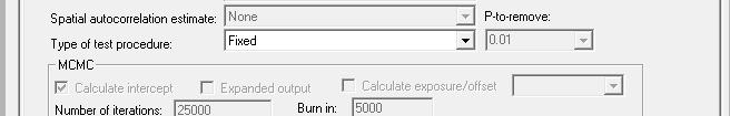
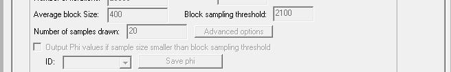
91 Fgure Up. 2.10: Regresson I Setup Page

92 dependent varable. A keystroke trck s to clck on the frst letter of the varable that wll be the dependent varable and the routne wll go to the frst varable wth that letter. Independent Varables There s another box for defnng the ndependent varables. The user must choose one or more ndependent varables. In the routne, there s no lmt to the number. Keep n mnd that the varables are output n the same order as specfed n the dalogue so a user mght want to thnk how these should be dsplayed. Type of Dependent Varable There are fve optons that must be defned. The frst s the type of dependent varable: Normal (OLS) or Skewed (Posson). The default s a Posson. At ths pont, these are the only choces that are avalable though we wll be addng a bnomal and multnomal choce soon. Type of Dsperson Estmate The second opton that must be defned s the type of dsperson estmate to be used. The choces are Gamma, Posson, Posson wth lnear correcton (NB1), and Normal (automatcally defned for the OLS model). The default s Gamma. Soon, we wll be addng a log lnear and possbly another dsperson parameter to the routne. Type of Estmaton Method The thrd opton s the type of estmaton method to be used: Maxmum Lkelhood (MLE) or Markov Chan Monte Carlo (MCMC). The default s MLE. These methods were dscussed above and n appendces C and D. Spatal Autocorrelaton Estmate Fourth, f the user accepts an MCMC algorthm, then another choce s whether to run a spatal autocorrelaton estmate along wth t (a Condtonal Autoregressve functon, or CAR). Ths can only be run f the dependent varable s Posson and the dsperson parameter s Gamma. If the spatal autocorrelaton estmate s run, then the model becomes a Posson-Gamma-CAR whle f the spatal autocorrelaton estmate s not run the model remans a Posson-Gamma. Type of Test Procedure The ffth, and last opton, s whether to run a fxed model or a backward elmnaton stepwse procedure (only wth the normal or an MLE Posson model). Wth a fxed model, the total model s estmated and the coeffcents for each of the varables are estmated at the same tme. Wth the backward elmnaton stepwse procedure, all the varables n the model ntally but are removed one at a tme, based on the probablty level for remanng n the model. 87

93 If the fxed model s chosen, then all ndependent varables wll be regressed smultaneously. However, f the stepwse backward elmnaton procedure s selected, the user must defne a p-to-remove value. The choces are: 0.1, 0.05, 0.01, and The default s Tradtonally, 0.05 s used as a mnmal threshold for sgnfcance. We put n 0.01 to make the model strcter; wth the large datasets that typcally occur n polce departments, the less strct 0.05 crteron would not exclude many ndependent varables. But, the user can certanly use 0.05 nstead. MCMC Choces If the user chooses the MCMC algorthm to estmate ether a Posson-Gamma or a Posson- Gamma-CAR model, then several decsons have to be made. Number of Iteratons Specfy the number of teratons to be run. The default s 25,000. The number should be suffcent to produce relable estmates of the parameters. Check the MC Error/Standard devaton rato and the G-R statstc to be sure these are below 1.05 and 1.20 respectvely. Burn n Iteratons Specfy the number of ntal teratons that wll be dropped from the fnal dstrbuton (the burn n perod). The default s 5,000. The number of burn n teratons should be suffcent for the algorthm to reach an equlbrum state and produce relable estmates of the parameters. Check the MC Error/Standard devaton rato and the G-R statstc to be sure these are below 1.05 and 1.20 respectvely. Block Samplng Threshold The MCMC algorthm wll be run on all cases unless the number of records exceeds the number specfed n the block samplng threshold. The default s 6,000 cases. Note that f you run the MCMC for more cases than ths, calculatng tme wll ncrease substantally. For the non-spatal Posson-Gamma model, the ncrease s lnear. However, for the spatal Posson-Gamma model, the ncrease s exponental. Further, we have found that we cannot calculate the spatal model for more than about 6,000 cases. Average Block Sze Specfy the number of cases to be drawn n each block sample. The default s 400 cases. Note that ths s an average. Actual samples wll vary n sze. The output wll dsplay the expected sample sze and the average sample sze that was drawn. Number of Samples Drawn Specfy the number of samples to be drawn. The default s 25. We have found that relable estmates can be obtaned from 20 to 30 samples especally f the sequence converges quckly and even 88

94 10 samples can produce meanngful results. Obvously, the more samples that are drawn, the more relable wll be the fnal results. But, havng more samples wll not necessarly ncrease the precson beyond 30. Calculate Intercept The model can be run wth or wthout an ntercept (constant). The default s wth an ntercept estmated. To run the model wthout the ntercept, uncheck the Calculate ntercept box. Calculate Exposure/Offset If the model s a rsk or rate model (see equatons Up through Up. 2.78), then an exposure (offset) varable needs to be defned. Check the Calculate exposure/offset box and dentfy the varable that wll be used as the exposure varable. The coeffcent for ths varable wll automatcally be 1.0. Advanced Optons There s also a set of advanced optons for the MCMC algorthm. Fgure Up show the advanced optons dalogue. We would suggest keepng the default values ntally untl you become very famlar wth the routne. Intal Parameters Values The MCMC algorthm requres an ntal estmate for each parameter. There are default values that are used. For the beta coeffcents (ncludng the ntercept), the default values are 0. Ths assumes that the coeffcent s not sgnfcant and s frequently called a non-nformatve pror. These are dsplayed as a blank screen for the Beta box. However, estmates of the beta coeffcents can be substtuted for the assumed 0 coeffcents. To do ths, all ndependent varable coeffcents plus the ntercept (f used) must be lsted n the order n whch they appear n the model and must be separated by commas. Do not nclude the beta coeffcents for the spatal autocorrelaton, Φ, term (f used). For example, suppose there are three ndependent varables. Thus, the model wll have four coeffcents (the ntercept and the coeffcents for each of three ndependent varables). Suppose a pror study had been done n whch a Posson-Gamma model was estmated as: Y = e X1 2.1X X3 (Up. 2.80) The researcher wants to repeat ths model but wth a dfferent data set. The researcher assumes that the model usng the new data set wll have coeffcents smlar to the earler research. Thus, the followng would be specfed n the box for the betas under the advanced optons: 4.5, 0.3, -2.1, 3.4 (Up. 2.81) 89

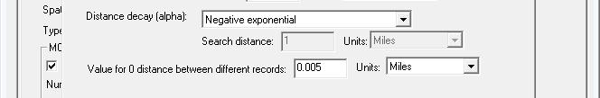
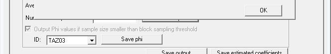
95 Fgure Up. 2.11: Advanced Optons for MCMC Posson-Gamma-CAR Model

96 The routne wll then use these values for the ntal estmates of the parameters before startng the MCMC process (wth or wthout the block samplng method). The advantage s that the dstrbuton wll converge more quckly (assumng the model s approprate for the new data set). Rho (ρ) and Tauph (τ ϕ ) The spatal autocorrelaton component, Φ, s made up of three separate sub-components, called Rho (ρ), Tauph (τ ϕ ), and Alpha (α, see formulas Up Up. 2.72). These are addtve. Rho s roughly a global component that apples to the entre data set. Tauph s roughly a neghborhood component that apples to a sub-set of the data. Alpha s essentally a localzed effect. The routne works by estmatng values for Rho and Tauph but uses a pre-defned value for Alpha. The default ntal values for Rho and Tauph are 0.5 and 1 respectvely. The user can substtute alternatve values for these parameters. Alpha(α) Alpha (α) s the exponent for the dstance decay functon n the spatal model. Essentally, the dstance decay functon defnes the weght to be appled to the values of nearby records. The weght can be defned by one of three mathematcal functons. Frst, the weght can be defned by a negatve exponental functon where Weght = e α*d(j) (Up. 2.82) where d(j) s the dstance between observatons and α s the value for alpha. It s automatcally assumed that alpha wll be negatve whether the user puts n a mnus sgn or not. The user nputs the alpha value n ths box. Second, the weght can be defned by a restrcted negatve exponental whereby the negatve exponental operates up to the specfed search dstance, whereupon the weght becomes 0 for greater dstances Up to Search dstance: Weght = e α*d(j) for d(j) 0, d(j) d p (Up. 2.83) Beyond search dstance: 0 for d(j) > d p (Up. 2.84) where d p s the search dstance. The coeffcent for the lnear component s assumed to be 1.0. Thrd, the weght can be defned as a unform value for all other observatons wthn a specfed search dstance. Ths s a contguty (or adjacency) measure. Essentally, all other observatons have an equal weght wthn the search dstance and 0 f they are greater than the search dstance. The user nputs the search dstance and unts n ths box. For the negatve exponental and restrcted negatve exponental functons, substtute the selected value for α n the alpha box. 91

97 Dagnostc Test for Reasonable Alpha Value The default functon for the weght s a negatve exponental wth a default alpha value of -1 n mles. For many data sets, ths wll be a reasonable value. However, for other data sets, t wll not. Reasonable values for alpha wth the negatve exponental functon are obtaned wth the followng procedure: 1. Decde on the measurement unts to be used to calculate alpha (mles, klometers, feet, etc). The default s mles. CrmeStat wll convert from the unts defned for the Prmary Fle nput dataset to those specfed by the user. 2. Calculate the nearest neghbor dstance from the Nna routne on the Dstance Analyss I page. These may have to be converted nto unts that were selected n step 1 above. For example, f the Nearest Neghbor dstance s lsted as 2000 feet, but the desred unts for alpha are mles, convert 2000 feet to mles by dvdng the 2000 by Input the dependent varable as the Z (ntensty) varable on the Prmary Fle page. 4. Run the Moran Correlogram routne on ths varable on the Spatal Autocorrelaton page (under Spatal Descrpton). By lookng at the values and the graph, decde whether the dstance decay n ths varable s very sharp (drops off quckly) or very shallow (drops off slowly). 5. Defne the approprate weght for the nearest neghbor dstance: a. Assume that the weght for an observaton wth tself (.e., dstance = 0) s 1.0. b. If the dstance decay drops off sharply, then a low weght for nearby values should be gven. Assume that any observatons at the nearest neghbor dstance wll only have a weght of 0.5 wth observatons further away beng even lower. c. If the dstance decay drops off more slowly, then a hgher weght for nearby values should be gven. Assume that any observatons at the nearest neghbor dstance wll have a weght of 0.9 wth observatons further away beng lower but only slghtly so. d. An ntermedate value for the weght s to assume t to be A range of alpha values can be solved usng these scenaros: a. For the sharp decay, alpha s gven by: α = ln(0.5)/nn(dstance) (Up. 2.85) 92

98 where NN(dstance) s the nearest neghbor dstance. b. For the shallow dstance decay, alpha s gven by: α = ln(0.9)/nn(dstance) (Up. 2.86) where NN(dstance) s the nearest neghbor dstance. c. For the ntermedate decay, alpha s gven by: α = ln(0.75)/nn(dstance) (Up. 2.87) where NN(dstance) s the nearest neghbor dstance. These calculatons wll provde a range of approprate values for α. The dagnostcs routne automatcally estmates these values as part of ts output. Value for 0 Dstances Between Records The advanced optons dalogue has a parameter for the mnmum dstance to be assumed between dfferent records. If two records have the same X and Y coordnates (whch could happen f the data are ndvdual events, for example), then the dstance between these records wll be 0. Ths could cause unusual calculatons n estmatng spatal effects. Instead, t s more relable to assume a slght dfference n dstance between all records. The default s mles but the user can modfy ths (ncludng substtutng 0 for the mnmal dstance). Output The output depends on whether an MLE or an MCMC model has been run. Maxmum Lkelhood (MLE) Model Output The MLE routnes (Normal, Posson, Posson wth lnear correcton, MLE Posson-Gamma) produce a standard output whch ncludes summary statstcs and estmates for the ndvdual coeffcents. MLE Summary Statstcs The summary statstcs nclude: Informaton About the Model 1. The dependent varable 2. The number of cases 3. The degrees of freedom (N number of parameters estmated) 93

99 4. The type of regresson model (Normal (OLS), Posson, Posson wth lnear correcton, Posson-Gamma) 5. The method of estmaton (MLE) Lkelhood Statstcs 6. Log lkelhood estmate, whch s a negatve number. For a set number of ndependent varables, the more negatve the log lkelhood the better. 7. Akake Informaton Crteron (AIC) adjusts the log lkelhood for the degrees of freedom. The smaller the AIC, the better. 8. Bayesan Informaton Crteron (BIC), sometmes known as the Schwartz Crteron (SC), adjusts the log lkelhood for the degrees of freedom. The smaller the BIC, the better. 9. Devance compares the log lkelhood of the model to the log lkelhood of a model that fts the data perfectly. A smaller devance s better. 10. The probablty value of the devance based on a Ch-square wth k-1 degrees of freedom. 11. Pearson Ch-square s a test of how closely the predcted model fts the data. A smaller Ch-square s better snce t ndcates the model fts the data well. Model Error Estmates 12. Mean Absolute Devaton (MAD). For a set number of ndependent varables, a smaller MAD s better. 13. Quartles for the Mean Absolute Devaton. For any one quartle, smaller s better. 14. Mean Squared Predctve Error (MSPE). For a set number of ndependent varables, a smaller MSPE s better. 15. Quartles for the Mean Squared Predctve Error. For any one quartle, smaller s better. 16. Squared multple R (for lnear model only). Ths s the percentage of the dependent varable accounted for by the ndependent varables. 17. Adjusted squared multple R (for lnear model only). Ths s the squared multple R adjusted for degrees of freedom. Over-dsperson Tests 18. Adjusted devance. Ths s a measure of the dfference between the observed and predcted values (the resdual error) adjusted for degrees of freedom. The smaller the adjusted devance, the better. A value greater than 1 ndcates over-dsperson. 19. Adjusted Pearson Ch-square. Ths s the Pearson Ch-square adjusted for degrees of freedom. The smaller the Pearson Ch-square, the better. A value greater than 1 ndcates over-dsperson. 20. Dsperson multpler. Ths s the rato of the expected varance to the expected mean. For a set number of ndependent varables, the smaller the dsperson multpler, the better. In a pure Posson dstrbuton, the dsperson should be 1.0. In practce, a rato greater than 10 ndcates that there s too much varaton that s unaccounted for n the model. Ether add more varables or change the functonal form of the model. 94

100 21. Inverse dsperson multpler. For a set number of ndependent varables, a larger nverse dsperson multpler s better. A rato close to 1.0 s consdered good. MLE Indvdual Coeffcent Statstcs For the ndvdual coeffcents, the followng are output: 22. The coeffcent. Ths s the estmated value of the coeffcent from the maxmum lkelhood estmate. 23. Standard Error. Ths s the estmated standard error from the maxmum lkelhood estmate. 24. Pseudo-tolerance. Ths s the tolerance value based on a normal predcton of the varable by the other ndependent varables. See equaton Up Z-value. Ths s asymptotc Z-test that s defned based on the coeffcent and standard error. It s defned as Coeffcent/Standard Error. 26. p-value. Ths s the two-tal probablty level assocated wth the Z-test. Markov Chan Monte Carlo (MCMC) Model Output The MCMC routnes (MCMC Posson-Gamma, Posson-Gamma-CAR) produce a standard output and an optonal expanded output. The standard output ncludes summary statstcs and estmates for the ndvdual coeffcents. MCMC Summary Statstcs The summary statstcs nclude: Informaton About the Model 1. The dependent varable 2. The number of records 3. The sample number. Ths s only output when the block samplng method s used. 4. The number of cases for the sample. Ths s only output when the block samplng method s used. 5. Date and tme for sample. Ths s only output when the block samplng method s used 6. The degrees of freedom (N number of parameters estmated) 7. The type of regresson model (Lnear, Posson, Posson wth lnear correcton, Posson- Gamma, Posson-Gamma-CAR) 8. The method of estmaton 9. The number of teratons 10. The burn n perod 11. The dstance decay functon used for a Posson-Gamma-CAR model. Ths s output wth the Posson-Gamma-CAR model only. 12. The block sze s the expected number of records selected for each block sample. The actual number may vary. 95

101 13. The number of samples drawn. Ths s output when the block samplng method used. 14. The average block sze. Ths s output when the block samplng method used. 15. The type of dstance decay functon. Ths s output for the Posson-Gamma-CAR model only. 16. Condton number for the dstance matrx. If the condton number s large, then the model may not have properly converged. Ths s output for the Posson-Gamma-CAR model only. 17. Condton number for the nverse dstance matrx. If the condton number s large, then the model may not have properly converged. Ths s output for the Posson-Gamma- CAR model only. Lkelhood Statstcs 18. Log lkelhood estmate, whch s a negatve number. For a set number of ndependent varables, the smaller the log lkelhood (.e., the most negatve) the better. 19. Devance Informaton Crteron (DIC) adjusts the log lkelhood for the effectve degrees of freedom. The smaller the DIC, the better. 20. Akake Informaton Crteron (AIC) adjusts the log lkelhood for the degrees of freedom. The smaller the AIC, the better. 21. Bayesan Informaton Crteron (BIC), sometmes known as the Schwartz Crteron (SC), adjusts the log lkelhood for the degrees of freedom. The smaller the BIC, the better. 22. Devance compares the log lkelhood of the model to the log lkelhood of a model that fts the data perfectly. A smaller devance s better. 23. The probablty value of the devance based on a Ch-square wth k-1 degrees of freedom. 24. Pearson Ch-square s a test of how closely the predcted model fts the data. A smaller Ch-square s better snce t ndcates the model fts the data well. Model Error Estmates 25. Mean Absolute Devaton (MAD). For a set number of ndependent varables, a smaller MAD s better. 26. Quartles for the Mean Absolute Devaton. For any one quartle, smaller s better. 27. Mean Squared Predctve Error (MSPE). For a set number of ndependent varables, a smaller MSPE s better. 28. Quartles for the Mean Squared Predctve Error. For any one quartle, smaller s better. Over-dsperson Tests 29. Adjusted devance. Ths s a measure of the dfference between the observed and predcted values (the resdual error) adjusted for degrees of freedom. The smaller the adjusted devance, the better. A value greater than 1 ndcates over-dsperson. 30. Adjusted Pearson Ch-square. Ths s the Pearson Ch-square adjusted for degrees of freedom. The smaller the Pearson Ch-square, the better. A value greater than 1 ndcates over-dsperson. 96

102 31. Dsperson multpler. Ths s the rato of the expected varance to the expected mean. For a set number of ndependent varables, the smaller the dsperson multpler, the better. In a pure Posson dstrbuton, the dsperson should be 1.0. In practce, a rato greater than 10 ndcates that there s too much varaton that s unaccounted for n the model. Ether add more varables or change the functonal form of the model. 32. Inverse dsperson multpler. For a set number of ndependent varables, a larger nverse dsperson multpler s better. A rato close to 1.0 s consdered good. MCMC Indvdual Coeffcent Statstcs For the ndvdual coeffcents, the followng are output: 33. The mean coeffcent. Ths s the mean parameter value for the N-k teratons where k s the burn n samples that are dscarded. Wth the MCMC block samplng method, ths s the mean of the mean coeffcents for all block samples. 34. The standard devaton of the coeffcent. Ths s an estmate of the standard error of the parameter for the N-k teratons where k s the burn n samples that are dscarded. Wth the MCMC block samplng method, ths s the mean of the standard devatons for all block samples. 35. t-value. Ths s the t-value based on the mean coeffcent and the standard devaton. It s defned by Mean/Std. 36. p-value. Ths s the two-tal probablty level assocated wth the t-test. 37. Adjusted standard error (Adj. Std). The block samplng method wll produce substantal varaton n the mean standard devaton, whch s used to estmate the standard error. Consequently, the standard error wll be too large. An approxmaton s made by multplyng the estmated standard devaton by where n s the average sample sze N of the block samples and N s the number of records. If no block samples are taken, then ths statstc s not calculated. 38. Adjusted t-value. Ths s the t-value based on the mean coeffcent and the adjusted standard devaton. It s defned by Mean/Adj_Std. If no block samples are taken, then ths statstc s not calculated. 39. Adjusted p-value. Ths s the two-tal probablty level assocated wth the adjusted t- value. If no block samples are taken, then ths statstc s not calculated. 40. MC error s a Monte Carlo smulaton error. It s a comparson of the means of m ndvdual chans relatve to the mean of the entre chan. By tself, t has lttle meanng. 41. MC error/std s the MC error dvded by the standard devaton. If ths rato s less than.05, then t s a good ndcator that the posteror dstrbuton has converged. 42. G-R stat s the Gelman-Rubn statstc whch compares the varance of m ndvdual chans relatve to the varance of the entre chan. If the G-R statstc s under 1.2, then the posteror dstrbuton s commonly consdered to have converged. n 97

103 43. Spatal autocorrelaton term (Ph, ϕ) for Posson-Gamma-CAR models only. Ths s the estmate of the fxed effect spatal autocorrelaton effect. It s made up of three components: a global component (Rho, ρ); a local component (Tauph, τ φ ); and a local neghborhood component (Alpha, α, whch s defned by the user). 44. The log of the error n the model (Taups). Ths s an estmate of the unexplaned varance remanng. Taups s the exponent of the dsperson multpler, e τψ. For any fxed number of ndependent varables, the smaller the Taups, the better. Expanded Output (MCMC Only) If the expanded output box s selected, addtonal nformaton on the percentles from the MCMC sample are dsplayed. If the block samplng method s used, the percentles are the means of all block samples. The percentles are: th percentle th percentle th percentle th percentle th percentle (medan) TH percentle th percentle th percentle th percentle The percentles can be used to construct confdence ntervals around the mean estmates or to provde a non-parametrc estmate of sgnfcance as an alternatve to the estmated t-value n the standard output. For example, the 2.5 th and 97.5 th percentles provde approxmate 95 percent confdence ntervals around the mean coeffcent whle the 0.5 th and 99.5 th percentles provde approxmate 99 percent confdence ntervals. The percentles wll be output for all estmated parameters ncludng the ntercept, each ndvdual predctor varable, the spatal effects varable (Ph), the estmated components of the spatal effects (Rho and Tauph), and the overall error term (Taups). Output Ph Values (Posson-Gamma-CAR Model Only) For the Posson-Gamma-CAR model only, the ndvdual Ph values can be output. Ths wll occur f the sample sze s smaller than the block samplng threshold. Check the Output Ph value f sample sze smaller than block samplng threshold box. An ID varable must be dentfed and a DBF output fle defned. 98

104 Save Output The predcted values and the resdual errors can be output to a DBF fle wth a REGOUT<root name> fle name where rootname s the name specfed by the user. The output s saved as a dbf fle under a dfferent fle name. The output ncludes all the varables n the nput data set plus two new ones: 1) the predcted values of the dependent varable for each observaton (wth the feld name PREDICTED); and 2) the resdual error values, representng the dfference between the actual /observed values for each observaton and the predcted values (wth the feld name RESIDUAL). The fle can be mported nto a spreadsheet or graphcs program and the errors plotted aganst the predcted dependent varable (smlar to fgure Up. 2.3). Save Estmated Coeffcents The ndvdual coeffcents can be output to a DBF fle wth a REGCOEFF<root name> fle name where rootname s the name specfed by the user. Ths fle can be used n the Make Predcton routne under Regresson II. Dagnostc Tests The regresson module has a set of dagnostc tests for evaluatng the characterstcs of the data and the most approprate model to use. There s a dagnostcs box on the Regresson I page (see fgure Up. 2.10). Dagnostcs are provded on: 1. The mnmum and maxmum values for the dependent and ndependent varables 2. Skewness n the dependent varable 3. Spatal autocorrelaton n the dependent varable 4. Estmated values for the dstance decay parameter alpha, for use n the Posson-Gamma- CAR model 5. Multcolnarty among the ndependent varables Mnmum and Maxmum Values for the Varables The mnmum and maxmum values of both the dependent and ndependent varables are lsted. A user should look for nelgble values (e.g., -1) as well as varables that have a very hgh range. The MLE routnes are senstve to varables wth very large ranges. To mnmze the effect, varables are nternally scaled when beng run (by dvdng by ther mean) and then re-scaled for output. Nevertheless, varables wth extreme ranges n values and especally varables where there are a few observatons wth extreme values can dstort the results for models. 7 A user would be better choosng a more balanced varable than usng one where one or two observatons determnes the relatonshp wth the dependent varable. 7 For example, n Excel, two columns of random numbers from 1 to 10 were lsted n 99 rows to represent two varables X1 and X2. The correlaton between these two varables over the 99 rows (observatons) was An addtonal row was added and the two varables gven a value of 100 each for ths row. Now, the correlaton between these two varables ncreased to 0.89! The pont s, one or two extreme values can dstort a statstcal relatonshp. 99

105 Skewness Tests As we have dscussed, skewness n a varable can dstort a normal model by allowng hgh values to be underestmated whle allowng low values to be overestmated. For ths reason, a Posson-type model s preferred over the normal for hghly skewed varables. The dagnostcs utlty tests for skewness usng two dfferent measures. Frst, the utlty outputs the g statstc (Mcrosoft, 2003): g n 3 [( X X ) / s] ( n 1)( n 2) (Up. 2.88) where n s the sample sze, X s observaton, X s the mean of X, and s s the sample standard devaton (corrected for degrees of freedom). The sample standard devaton s defned as: s ( X X ) ( n 1) 2 (Up. 2.89) The standard error of skewness (SES) can be approxmated by (Tabachnck and Fdell, 1996): SES 6 (Up. 2.90) n An approxmate Z-test can be obtaned from: g Z( g) (Up. 2.91) SES Thus, f Z s greater than or smaller than -1.96, then the skewness s sgnfcant at the p.05 level. An example s the number of crmes orgnatng n each traffc analyss zone wthn Baltmore County n The summary statstcs were: X = s = n = 325 Therefore, 3 [( X X ) / s]

106 325 g * * SES Z ( g) The Z of the g value shows the data are hghly skewed. The second skewness measure s a rato of the smple varance to the smple mean. Whle ths rato had not been adjusted for any predctor varables, t s usually a good ndcator of skewness. Ratos greater than about 2:1 should make the user cautous about usng a normal model. If ether measure ndcates skewness, CrmeStat prnts out a message ndcatng the dependent varable appears to be skewed and that a Posson or Posson-Gamma model should be used. Testng for Spatal Autocorrelaton n the Dependent Varable The thrd type of test n the dagnostcs utltes s the Moran s I coeffcent for spatal autocorrelaton. The statstc was dscussed extensvely n chapter 4. If the I s sgnfcant, CrmeStat outputs a message ndcatng that there s defnte spatal autocorrelaton n the dependent varable and that t needs to be accounted for, ether by a proxy varable or by estmatng a Posson-Gamma-CAR model. A proxy varable would be one that can capture a substantal amount of the prmary reason for the spatal autocorrelaton. One such varable that we have found to be very useful s the dstance of the locaton from the metropoltan center (e.g., downtown). Almost always, populaton denstes are much hgher n the central cty than n the suburbs, and ths dfferental n densty apples to most phenomena ncludng crme (e.g., populaton densty, employment densty, traffc densty, events of all types). It represents a frst-order spatal effect, whch was dscussed n chapters 4 and 5 and s the result of other processes. Another proxy varable that can be used s ncome (e.g., medan household ncome, medan ndvdual ncome) whch tends to account for much clusterng n an urban area. The problem wth ncome as a proxy varable s that t s both causatve (ncome determnes spatal locaton) as well as a byproduct of populaton denstes. The combnaton of both ncome and dstance from the metropoltan center can capture most of the effect of spatal autocorrelaton. An alternatve s to use the Posson-Gamma-CAR model to flter out some of the spatal autocorrelaton. As we dscussed above, ths s useful only when all obvous spatal effects have already been ncorporated nto the model. A sgnfcant spatal effect only means that the model cannot explan the addtonal clusterng of the dependent varable. 101

107 Estmatng the Value of Alpha (α) for the Posson-Gamma-CAR Model The fourth type of test produced by the dagnostcs utlty s an estmate of a plausble value for the dstance decay functon alpha, α, n the Posson-Gamma-CAR model. The way the estmate s produced was dscussed above and s based on assgnng a proportonal weght for the dstance assocated wth the nearest neghbor dstance, the average dstance from each observaton to ts nearest neghbor (see chapter 6). Three values of α are gven n dfferent dstance unts, one assocated wth a weght of 0.9 ( a very steep dstance decay, one assocated wth a weght of 0.75 (a moderate dstance decay), and one assocated wth a weght of 0.5 (a shallow dstance decay). Users should run the Moran Correlogram and examne the gra ph of the drop off n spatal autocorrelaton to assess what type of decay functon most lkely exsts. The user should choose an α value that best represents the dstance decay and should defne the dstance unts for t. Multcollnearty Tests The ffth type of dagnostc test s for multcollnearty among the ndependent predctors. As we have dscussed n ths chapter, one of the major problems wth many regresson models, whether MLE or MCMC, s multcollnearty among the ndependent varables. To assess multcollnearty, the pseudo-tolerance test s presented for each ndependent varable. Ths was dscussed above n the chapter (see equaton Up. 2.18). Lkelhood Ratos One test that we have not mplemented n the regresson I module s the lkelhood rato because t s so smple. A lkelhood rato s the rato of the log lkelhood of one model to that of another. For example, a Posson-Gamma model run wth three ndependent varables can be compared wth a Posson- Gamma model wth two ndependent varables to see f the thrd ndependent varable sgnfcantly adds to the predcton. The test s very smple. Let L C be the log lkelhood of the comparson model and let L B be the log lkelhood of the baselne model (the model to whch the comparson model s beng compared). Then, LR = 2(L C L B ) (Up. 2.92) 2 LR s dstrbuted as a statstc wth K degrees of freedom where K s the dfference n the number of parameters estmated between the two models ncludng the ntercepts. In the example above, K s 1 snce a model wth three ndependent varables plus an ntercept (d.f. = 4) s beng compared wth a model wth two ndependent varables plus an ntercept (d.f.=3). 102

108 Regresson II Module The Regresson II module allows the user to apply a model to another dataset and make a predcton. Fgure Up show the Regresson II setup page. The Make predcton routne allows the applcaton of coeffcents to a dataset. Note that, n ths case, the coeffcents are beng appled to a dfferent Prmary Fle than that from whch they were calculated. For example, a model mght be calculated that predcts robberes for The saved coeffcent fle then s appled to another dataset, for example robberes for There are two types of models that are ftted normal and Posson. For the normal model, the routne fts the equaton: Y = β 0 + β 1 X β k X k (Up. 2.93) whereas for the Posson model, the routne fts the equaton: E(Y / X k ) = λ = e β0 + β1x βkxk + [Φ] (Up. 2.94) wth β 0 beng the ntercepted (f calculated), β 1. β k beng the saved coeffcents and Φ s the saved Ph values (f the Posson-Gamma-CAR model was estmated). Notce that there s no error n each equaton. Error was part of the estmaton model. What were saved was only the coeffcents. For both types of model, the coeffcents fle must nclude nformaton on the ntercept and each of the coeffcents. The user reads n the saved coeffcent fle and matches the varables to those n the new dataset based on the order of the coeffcents fle. If the model had estmated a general spatal effect from a Posson-Gamma-CAR model, then the general Φ wll have been saved wth the coeffcent fles. If the model had estmated specfc spatal effects from a Posson-Gamma-CAR model, then the specfc Φ values wll have been saved n a separate Ph coeffcents fle. In the latter case, the user must read n the Ph coeffcents fle along wth the general coeffcent fle. 103

109 Fgure Up. 2.12: Regresson II Setup Page