Standard Normal, Inverse Normal and Sampling Distributions
|
|
|
- Simon Gallagher
- 5 years ago
- Views:
Transcription
1 Standard Normal, Inverse Normal and Sampling Distributions Section 5.5 & 6.6 Cathy Poliak, Ph.D. Office in Fleming 11c Department of Mathematics University of Houston Lecture Cathy Poliak, Ph.D. Office in Fleming 11c Section (Department 5.5 & 6.6of Mathematics University of Houston Lecture ) / 56
2 Outline 1 Using the z-table 2 Inverse Normal 3 Sums of Random Variables 4 Sampling Distributions 5 Sampling Distribution of X 6 Finding Probabilities for X 7 Approximating the Binomial Distribution 8 Proportions 9 Sampling Distribution of ˆp Cathy Poliak, Ph.D. cathy@math.uh.edu Office in Fleming 11c Section (Department 5.5 & 6.6of Mathematics University of Houston Lecture ) / 56
3 Introduction Questions Let a random variable X have a Normal distribution with mean µ = 10 and standard deviation σ = 2. For the following questions determine what is the proper way to solve these probabilities. 1. P(X < 7.25) 2. P(X 5) a) pnorm(7.25,10,2) c) pnorm(7,10,2) b) 1-pnorm(7.25,10,2) d) dnorm(7.25, 10, 2) a) pnorm(5, 10, 2) c) 1 - pnorm(4, 10, 2) b) 1 - pnorm(5, 10, 2) d) dnorm(6, 10, 2) 3. P(9 X 11) a) pnorm(11, 10, 2) - pnorm(8, 10, 2) b) pnorm(11, 10, 2) - 1- pnorm(9, 10, 2) c) pnorm(11, 10, 2) - pnorm(9, 10, 2) d) dnorm(11, 10, 2) - dnorm(9, 10, 2) Cathy Poliak, Ph.D. cathy@math.uh.edu Office in Fleming 11c Section (Department 5.5 & 6.6of Mathematics University of Houston Lecture ) / 56
4 Normal Distribution Calculations Area under a Normal curve represent proportions (probability) of observations within a range of values. There is no easy way to find the area under a Normal curve. We use a table or software that calculates the desired areas. The table we use is Z-table It uses a cumulative proportion. A cumulative proportion is the proportion (probability) of observations in a distribution that lie at or below a given value. This is Φ(z). When the distribution is given by a density curve, the cumulative proportion is the area under the curve to the left of a given value. Cathy Poliak, Ph.D. cathy@math.uh.edu Office in Fleming 11c Section (Department 5.5 & 6.6of Mathematics University of Houston Lecture ) / 56
5 Using The Z-table The vertical margin are the left most digits of a z-score. The top margin is the hundredths place of a z-score. The numbers inside the table represents the area from to that z-score. Remember that the standard Normal density curve is symmetric and the total area is equal to 1. Note: R can calculate these probabilities and also some calculators. Without having to convert to z-scores. Cathy Poliak, Ph.D. cathy@math.uh.edu Office in Fleming 11c Section (Department 5.5 & 6.6of Mathematics University of Houston Lecture ) / 56
6 P(Z 1.52) P(Z -1.52) Cathy Poliak, Ph.D. Office in Fleming 11c Section (Department 5.5 & 6.6of Mathematics University of Houston Lecture ) / 56
 Cathy Poliak, Ph.D. cathy@math.uh.edu Office in Fleming 11c Section (Department 5.5 & 6.")
7 P(Z 1.52) = R: pnorm(-1.52) = Table A: P(Z < z) z P(Z -1.52) Cathy Poliak, Ph.D. cathy@math.uh.edu Office in Fleming 11c Section (Department 5.5 & 6.6of Mathematics University of Houston Lecture ) / 56
8 P(Z 0.95) P(Z 0.95) Cathy Poliak, Ph.D. Office in Fleming 11c Section (Department 5.5 & 6.6of Mathematics University of Houston Lecture ) / 56
9 P(Z 0.95) = R: 1 - pnorm(0.95) = Table A: P(Z < z) z P(Z 0.95)= 1 P( Z < 0.95) = = Cathy Poliak, Ph.D. cathy@math.uh.edu Office in Fleming 11c Section (Department 5.5 & 6.6of Mathematics University of Houston Lecture ) / 56

10 P(1.3 < Z < 1.72) P(1.3 < Z < 1.72) / 56
11 P(1.3 < Z < 1.72) = R: pnorm(1.72) - pnorm(1.3) = z P(1.3 < Z < 1.72) = = / 56
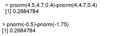
 that less than 5 ounces of")
 that between 4 and 4.")
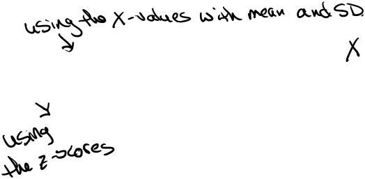
12 Example Let X = amount of juice in ounces in a orange, X N(4.7, 0.4). 1. Determine the probability (using the z-table) that less than 5 ounces of juice are in an orange. 2. Determine the probability (using the z-table) that between 4 and 4.5 ounces of juice are in an orange / 56
13
14 Finding a value when given a proportion Called inverse Normal. This is working Backwards using Z-Table. Finding the observed values when given a percent. In R: qnorm(proportion,mean,sd) / 56
15 Backward Normal calculations Using Z-Table 1. State the problem. Since, Z-Table and qnorm are based on the areas to the left of z-scores or x-scores, always state the problem in terms of the area to the left of x. Keep in mind that the total area under the standard Normal curve is Use Table A to find c. This is the value from the table not a value that we calculate. 3. Unstandardized to transform the solution from the z-score back to the original x scale. Solving for x using the equation gives the equation x = σ(c) + µ. c = x µ σ / 56


 = 0.006 3.")
16 Examples to Work "Backwards" with the Normal Distribution Find the value of c so that: 1. P(Z < c) = P(Z > c) = P( c < Z < c) = / 56
17
18 MPG for Prius The miles per gallon for a Toyota Prius has a Normal distribution with mean µ = 49 mpg and standard deviation σ = 3.5 mpg. 25% of the Prius have a MPG of what value and lower? 1. We want c, such that P(Z < c) = That is we want to know what z-score cuts off the lowest 25%. P( Z <?) =0.25 z / 56
19 Find c such that P(Z < c) = From Table A, find something close to 0.25 inside the table. z P(Z <?) = 0.25 (closes value is ) z = (-0.6 row column ) / 56
20 Find c such that P(Z < c) = Unstandardized: x = σ(c) + µ = 3.5( 0.67) + 49 = This means that 25% of the Prius has a mpg of less than mpg. Using R: qnorm(0.25,49,3.5) = / 56


21 Top 10% Suppose you rank in the 10% of your class. If the mean GPA is 2.7 and the standard deviation is 0.59, what is your GPA? ( Assume a Normal distribution) 1. We want c, such that P(Z > c) = That is we want to know what z-score cuts off the highest 10%. P(Z >?) = 0.10 z / 56
22 Find c such that P(Z > c) = From Table A, the areas are below or to the left of a z-score thus we want to find something close to 0.90 inside the table. z P(Z <?) = 0.90 (close value is ) z = 1.28 (1.2 row column ) / 56
23 Find c such that P(Z > c) = Unstandardized: x = σ(c) + µ = 0.59(1.28) = This means that your gpa is if you rank at the 10% of your class. In R: qnorm(0.9,2.7,0.59) = / 56

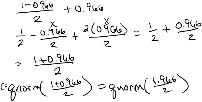
24 Example Let X = amount of juice in ounces in a orange, X N(4.7, 0.4). 1. Determine the third quartile. 2. Determine the 95th percentile / 56
25 Recall E(X + Y ) If X and Y are two different random variables, then the expected value (mean) of the sums of the pairs of the random variable is the same as the sum of their means: µ X+Y = E(X + Y ) = E(X) + E(Y ) = µ X + µ Y. This is called the addition rule for means. The expected value (mean) of the difference of the pairs of the random variable is the same as the difference of their means: µ X Y = E(X Y ) = E(X) E(Y ) = µ X µ y / 56
 + Var(Y ) = σ2 X + σ2 Y σ 2 X Y = Var(X Y ) = Var(X) + Var(Y ) = σ2 X + σ2 Y - 3339 24")
26 Recall VAR(X + Y ) If X and Y are independent random variables and σ 2 X+Y = Var(X + Y ) = Var(X) + Var(Y ) = σ2 X + σ2 Y σ 2 X Y = Var(X Y ) = Var(X) + Var(Y ) = σ2 X + σ2 Y / 56
27 If X & Y are dependent If X and Y are dependent random variables then σx+y 2 = Var(X + Y ) = Var(X)+Var(Y ) + 2cov(X, Y ) = σx 2 + σy 2 + 2cov(X, Y ) and σx Y 2 = Var(X Y ) = Var(X)+Var(Y ) 2cov(X, Y ) = σx 2 + σy 2 2cov(X, Y ) / 56

28 Example Suppose we have two independent random variables, X and Y where µ X = 10, σ X = 2, µ Y = 10 and σ Y = 2. a. Determine: µ X+Y and σ X+Y b. Suppose we want the mean of X and Y, what would be the expected value of the mean? / 56
29 Popper 12 Questions Consider one family as a population of five children. We are looking at the ages of these five children: 3, 5, 9, 11, Determine the population mean, µ, age of these children. a. 9 b. 10 c. 8.4 d Determine the population standard deviation, σ, of these children. a. 10 b. 4 c Suppose we take a sample of 2 children from this population. What would we expect the sample mean, x from the 2 children to be? a. 2 b. 8.4 c. 4 d / 56
 4 (3,9) 6 (3,11) 7 (3, 14) 8.5 (5, 9) 7 (5, 11) 8 (5, 14) 9.5 (9, 11) 10 (9, 14) 11.5 (11, 14) 12.")
30 Sampling Distribution of size 2 From the five children, we want to list out all possible pairs of size 2 and determine their mean. Ages are: 3,5, 9, 11, 14 Pairs Sample mean, x (3,5) 4 (3,9) 6 (3,11) 7 (3, 14) 8.5 (5, 9) 7 (5, 11) 8 (5, 14) 9.5 (9, 11) 10 (9, 14) 11.5 (11, 14) 12.5 The list above is a sampling distribution from a sample of 2 of x, the possible values of the sample mean. What is the mean of the sample means, µ x? What is the standard deviation of the sample means, σ x? / 56
 9.3333 (5, 9, 11) 8.3333 (5, 9, 14) 9.3333 (5, 11, 14) 10 (9, 11, 14) 11.3333 What is the mean of these means, µ x? What is the standard deviation of these means, σ x?")
31 Sampling Distribution of size 3 What about the sampling distribution of size 3 from the family of five? Sets x (3, 5, 9) (3, 5, 11) (3, 5, 14) (3, 9, 11) (3, 9, 14) (3, 11, 14) (5, 9, 11) (5, 9, 14) (5, 11, 14) 10 (9, 11, 14) What is the mean of these means, µ x? What is the standard deviation of these means, σ x? / 56
32 Sampling distribution When we describe distributions we use three characteristics: Shape Center Spread To describe the sampling distribution we can use the same three characteristics. This can be shown through histograms or numerical values / 56
33 Sampling Distribution of X Suppose that X is the sample mean of a simple random sample of size n from a large population with mean µ and standard deviation σ. X is a random variable because every time we take a random sample we will not get the same sample mean X. Thus we want to know the distribution of the sample means X. The center of the sample means (mean of the sample means) µ X is µ. Also called the expected value. The spread of the sample means (standard deviation of the sample means) σ X is σ/ n / 56

34 Sampling Distribution Example Assume that cans of Pepsi are filled so that the actual amount have a mean µ = 12 oz and a standard deviation σ = 0.09 oz. We take a sample of 25 cans and find the mean amount X in these 25 cans. What would we expect the mean to be? Would the sample mean be exactly that value? If not how far off could the sample mean be? / 56


35 Sampling Distribution Example Assume that cans of Pepsi are filled so that the actual amount have a mean µ = 12 oz and a standard deviation σ = 0.09 oz. We take a sample of 100 cans and find the mean amount X in these 100 cans. What would we expect the mean to be? Would the sample mean be exactly that value? If not how far off could the sample mean be? / 56
36 Shape of the Sample Mean Distribution If a population has a Normal distribution, then the sample mean X of n independent observations also has a Normal distribution with mean µ and standard deviation σ/ n. Central limit theorem: For any population, when n is large (n > 30), the sampling distribution of the sample mean X is approximately a Normal distribution with mean µ and standard deviation σ/ n / 56

37 Example: Amount of Pepsi Assume that cans of Pepsi are filled so that the actual amount have a mean µ = 12 oz and a standard deviation σ = 0.09 oz. Suppose that a random sample of 4 cans are examined, describe the distribution of the sample means X. Center: µ X = µ = 12 Spread: σ X = σ n = = Shape: Unknown because we do not know the original distribution and the sample size is small / 56
38 Example: Amount of Pepsi Assume that cans of Pepsi are filled so that the actual amount have a mean µ = 12 oz and a standard deviation σ = 0.09 oz. Suppose that a random sample of 100 cans are examined, describe the distribution of the sample means X. Center: µ X = µ = 12 Spread: σ X = σ n = = Shape: Normal because we have a large sample thus we can apply the Central Limit Theorem / 56


39 Finding Probabilities Assume that cans of Pepsi are filled so that the actual amount have a mean µ = 12 oz and a standard deviation σ = 0.09 oz. Suppose that a random sample of 36 cans are examined, determine the probability that a sample of 36 cans will have a sample mean amount, X of at least oz. To find this probability we need to first describe the distribution: Shape: Normal because of the Central Limit Theorem Center: E[ X] = µ x = µ = 12 Spread: SD[ X] = σ x = σ/ n = 0.09/ 36 = this is the standard deviation we use. We want to know: P( X 12.01) / 56
40 Notes about finding probabilities for X We have a sample size n. Thus the standard deviation changes by that value SD( X) = σ X = σ n. The mean stays the same. mean( X) = µ X = µ. If we know that the original distribution is Normal or we have a large enough sample (n > 30). We can use the Normal distributions to find the probabilities / 56

41 Orange Juice An orange juice producer buys all his oranges from a large orange grove. The amount of juice squeezed from each of these oranges is approximately normally distributed, with a mean of 4.70 ounces and a standard deviation of 0.40 ounce. Suppose we take a random sample of 4 oranges and determine the mean of this sample, X. 1. What is the shape of the sampling distribution of X. 2. What is the mean of the sampling distribution of X. 3. What is the standard deviation of the sampling distribution of X. 4. What is the probability that the sample mean of the 4 oranges will be at 4.5 or less? / 56
42
43 Approximation for Binomial Suppose a random variable X has a binomial distribution with p = 0.1. The following is a histogram with n = 10. n = 10, p= 0.1 Density / 56
44 Approximation for Binomial Suppose a random variable X has a binomial distribution with p = 0.1. The following is a histogram with n = 20. n = 20, p= 0.1 Density / 56
45 Approximation for Binomial Suppose a random variable X has a binomial distribution with p = 0.1. The following is a histogram with n = 50. n = 50, p= 0.1 Density / 56
46 Approximation for Binomial Suppose a random variable X has a binomial distribution with p = 0.1. The following is a histogram with n = 100. n = 100, p= 0.1 Density / 56
47 Theorem 5.3 Let X be a binomial random variable based on n trials with success probability p. Then if the binomial probability histogram is not too skewed, X has an approximate Normal distribution with µ = np and σ = np(1 p). In particular, for x = a possible value of X, P(X x) = Binom(x; n, p) (area under the normal curve to the left of x + 0.5) ( ) x np = Φ np(1 p) In practice, the approximate is adequate provided that both np 10 and n(1 p) / 56

48 Example of Normal Approximation Suppose that your mail-order company advertises that it ships 90% of its orders within three working days. Suppose you take a simple random sample of 100 orders: 1. What is the probability that 86 or fewer of the orders are shipped on time? 2. What is the probability that more than 95 of the orders are shipped on time? / 56
49 Sample Proportions The population proportion is p a parameter. In some cases we do not know the population proportion, thus we use the sample proportion, ˆp to estimate p. The sample proportion is calculated by: ˆp = X n X = the number of observations of interest in the sample or the number of "successes" in the sample. n = the sample size or number of observations / 56

50 Example According to the National Retail Federation, 34% of taxpayers used computer software to do their taxes. A sample of 50 taxpayers was selected what do we expect the sample proportion ˆp to be? Of we take other samples will the sample proportions always be the same value? If not what would ˆp be off by? / 56

51 Sample Distribution of n = / 56
52 Sample Distribution of n = / 56
53 Shape of the distribution of ˆp Notice from the previous histograms that it appears to have a Normal distribution. We can use the Normal distribution as long as np 10 the number of successes are at least 10 and n(1 p) 10 the number of failures are at least / 56
54 Center of the distribution of ˆp The center is the mean (expected value): µˆp = p the proportion of success. ˆp = X n where X is the number of successes out of n observations. Thus X has a binomial distribution with parameters n and p. The mean of X is: µ X = E(X) = np Thus by rule 1b for means, the mean of ˆp is: ( ) X µˆp = E(ˆp) = E = µ X n n = np n = p / 56
55 Spread of the distribution of ˆp The spread is the standard deviation σˆp = The variance of X is: p(1 p) n. σ 2 X = Var(X) = np(1 p) By rule 1b for variance, the variance of ˆp is: ( ) X σ 2ˆp = Var (ˆp) = Var = Var(X) np(1 p) p(1 p) n n 2 = n 2 = n athy Poliak, Ph.D. cathy@math.uh.edu Office in Fleming 11c Section (Department 5.5 & 6.6of Mathematics University of Lecture Houston 9) / 56
 at least 10.")
56 Assumptions The sampled values must be random and independent of each other. This can be tested by 10% Condition: The sample size must be no larger than 10% of the population. The sample size, n must be large enough. This can be be tested by Success / Failure Condition: The sample size has to be big enough so that both np and n(1 p) at least / 56
57 Example for distribution of ˆp According to the National Retail Federation, 34% of taxpayers used computer software to do their taxes. A sample of 125 taxpayers was selected. What is the distribution of ˆp, the sample proportion of the 125 taxpayers that used computer software to do their taxes? 1. Check if we can use the Normal distribution. p = 0.34, n = 125 np = 125(0.34) = 42.5 n(1 p) = 125(1 0.34) = 125(0.66) = 82.5 Both np and n(1 p) are greater than 10 so we can use the Normal distribution. 2. The mean is: µˆp = p = If we take a sample we "expect" 34% to have used computer software to do their taxes. 3. The standard deviation is: σˆp = p(1 p) n = 0.34(1 0.34) 125 = / 56
58 Example continued According to the National Retail Federation, 34% of taxpayers used computer software to do their taxes. A sample of 125 taxpayers was selected. What is the probability that between 28% and 40% of the taxpayers from the sample of 125 used computer software to do their taxes? 1. We want: P(0.28 < ˆp < 0.40) / 56

59 Facebook Example The Social Media and Personal Responsibility Survey in 2010 found the 69% of parents are "friends" with their children on Facebook. A random sample of 140 parents was selected and we determined the proportion of parents from this sample, ˆp that are "friends" with their children on Facebook. 1. What is the shape of the sampling distribution of ˆp. 2. What is the mean of the sampling distribution of ˆp. 3. What is the standard deviation of the sampling distribution of ˆp. 4. What is the probability that the sample proportion of 140 parents is greater than 72%? / 56
Inverse Normal Distribution and Approximation to Binomial
 Inverse Normal Distribution and Approximation to Binomial Section 5.5 Cathy Poliak, Ph.D. cathy@math.uh.edu Office in Fleming 11c Department of Mathematics University of Houston Lecture 16-3339 Cathy Poliak,
Standard Normal Calculations
 Standard Normal Calculations Section 4.3 Cathy Poliak, Ph.D. cathy@math.uh.edu Office in Fleming 11c Department of Mathematics University of Houston Lecture 10-2311 Cathy Poliak, Ph.D. cathy@math.uh.edu
Statistics for Business and Economics
 Statistics for Business and Economics Chapter 5 Continuous Random Variables and Probability Distributions Ch. 5-1 Probability Distributions Probability Distributions Ch. 4 Discrete Continuous Ch. 5 Probability
Normal Distribution. Notes. Normal Distribution. Standard Normal. Sums of Normal Random Variables. Normal. approximation of Binomial.
 Lecture 21,22, 23 Text: A Course in Probability by Weiss 8.5 STAT 225 Introduction to Probability Models March 31, 2014 Standard Sums of Whitney Huang Purdue University 21,22, 23.1 Agenda 1 2 Standard
Lecture 6: Chapter 6
 Lecture 6: Chapter 6 C C Moxley UAB Mathematics 3 October 16 6.1 Continuous Probability Distributions Last week, we discussed the binomial probability distribution, which was discrete. 6.1 Continuous Probability
Lecture 23. STAT 225 Introduction to Probability Models April 4, Whitney Huang Purdue University. Normal approximation to Binomial
 Lecture 23 STAT 225 Introduction to Probability Models April 4, 2014 approximation Whitney Huang Purdue University 23.1 Agenda 1 approximation 2 approximation 23.2 Characteristics of the random variable:
Lecture Slides. Elementary Statistics Tenth Edition. by Mario F. Triola. and the Triola Statistics Series. Slide 1
 Lecture Slides Elementary Statistics Tenth Edition and the Triola Statistics Series by Mario F. Triola Slide 1 Chapter 6 Normal Probability Distributions 6-1 Overview 6-2 The Standard Normal Distribution
Binomal and Geometric Distributions
 Binomal and Geometric Distributions Sections 3.2 & 3.3 Cathy Poliak, Ph.D. cathy@math.uh.edu Office in Fleming 11c Department of Mathematics University of Houston Lecture 7-2311 Cathy Poliak, Ph.D. cathy@math.uh.edu
Section Introduction to Normal Distributions
 Section 6.1-6.2 Introduction to Normal Distributions 2012 Pearson Education, Inc. All rights reserved. 1 of 105 Section 6.1-6.2 Objectives Interpret graphs of normal probability distributions Find areas
The Normal Probability Distribution
 1 The Normal Probability Distribution Key Definitions Probability Density Function: An equation used to compute probabilities for continuous random variables where the output value is greater than zero
Section 7.5 The Normal Distribution. Section 7.6 Application of the Normal Distribution
 Section 7.6 Application of the Normal Distribution A random variable that may take on infinitely many values is called a continuous random variable. A continuous probability distribution is defined by
ECON 214 Elements of Statistics for Economists 2016/2017
 ECON 214 Elements of Statistics for Economists 2016/2017 Topic The Normal Distribution Lecturer: Dr. Bernardin Senadza, Dept. of Economics bsenadza@ug.edu.gh College of Education School of Continuing and
Math 227 Elementary Statistics. Bluman 5 th edition
 Math 227 Elementary Statistics Bluman 5 th edition CHAPTER 6 The Normal Distribution 2 Objectives Identify distributions as symmetrical or skewed. Identify the properties of the normal distribution. Find
ECO220Y Continuous Probability Distributions: Normal Readings: Chapter 9, section 9.10
 ECO220Y Continuous Probability Distributions: Normal Readings: Chapter 9, section 9.10 Fall 2011 Lecture 8 Part 2 (Fall 2011) Probability Distributions Lecture 8 Part 2 1 / 23 Normal Density Function f
Data Analysis and Statistical Methods Statistics 651
 Data Analysis and Statistical Methods Statistics 651 http://www.stat.tamu.edu/~suhasini/teaching.html Suhasini Subba Rao The binomial: mean and variance Recall that the number of successes out of n, denoted
Chapter 6. The Normal Probability Distributions
 Chapter 6 The Normal Probability Distributions 1 Chapter 6 Overview Introduction 6-1 Normal Probability Distributions 6-2 The Standard Normal Distribution 6-3 Applications of the Normal Distribution 6-5
LECTURE 6 DISTRIBUTIONS
 LECTURE 6 DISTRIBUTIONS OVERVIEW Uniform Distribution Normal Distribution Random Variables Continuous Distributions MOST OF THE SLIDES ADOPTED FROM OPENINTRO STATS BOOK. NORMAL DISTRIBUTION Unimodal and
Binomial and Geometric Distributions
 Binomial and Geometric Distributions Section 3.2 & 3.3 Cathy Poliak, Ph.D. cathy@math.uh.edu Office hours: T Th 2:30 pm - 5:15 pm 620 PGH Department of Mathematics University of Houston February 11, 2016
Review of the Topics for Midterm I
 Review of the Topics for Midterm I STA 100 Lecture 9 I. Introduction The objective of statistics is to make inferences about a population based on information contained in a sample. A population is the
Week 7. Texas A& M University. Department of Mathematics Texas A& M University, College Station Section 3.2, 3.3 and 3.4
 Week 7 Oğuz Gezmiş Texas A& M University Department of Mathematics Texas A& M University, College Station Section 3.2, 3.3 and 3.4 Oğuz Gezmiş (TAMU) Topics in Contemporary Mathematics II Week7 1 / 19
Chapter 6 Continuous Probability Distributions. Learning objectives
 Chapter 6 Continuous s Slide 1 Learning objectives 1. Understand continuous probability distributions 2. Understand Uniform distribution 3. Understand Normal distribution 3.1. Understand Standard normal
Introduction to Statistics I
 Introduction to Statistics I Keio University, Faculty of Economics Continuous random variables Simon Clinet (Keio University) Intro to Stats November 1, 2018 1 / 18 Definition (Continuous random variable)
CH 5 Normal Probability Distributions Properties of the Normal Distribution
 Properties of the Normal Distribution Example A friend that is always late. Let X represent the amount of minutes that pass from the moment you are suppose to meet your friend until the moment your friend
Lecture 12. Some Useful Continuous Distributions. The most important continuous probability distribution in entire field of statistics.
 ENM 207 Lecture 12 Some Useful Continuous Distributions Normal Distribution The most important continuous probability distribution in entire field of statistics. Its graph, called the normal curve, is
Chapter 4 Continuous Random Variables and Probability Distributions
 Chapter 4 Continuous Random Variables and Probability Distributions Part 2: More on Continuous Random Variables Section 4.5 Continuous Uniform Distribution Section 4.6 Normal Distribution 1 / 28 One more
STA258H5. Al Nosedal and Alison Weir. Winter Al Nosedal and Alison Weir STA258H5 Winter / 41
 STA258H5 Al Nosedal and Alison Weir Winter 2017 Al Nosedal and Alison Weir STA258H5 Winter 2017 1 / 41 NORMAL APPROXIMATION TO THE BINOMIAL DISTRIBUTION. Al Nosedal and Alison Weir STA258H5 Winter 2017
Chapter 4 Continuous Random Variables and Probability Distributions
 Chapter 4 Continuous Random Variables and Probability Distributions Part 2: More on Continuous Random Variables Section 4.5 Continuous Uniform Distribution Section 4.6 Normal Distribution 1 / 27 Continuous
Elementary Statistics Lecture 5
 Elementary Statistics Lecture 5 Sampling Distributions Chong Ma Department of Statistics University of South Carolina Chong Ma (Statistics, USC) STAT 201 Elementary Statistics 1 / 24 Outline 1 Introduction
Lecture 8. The Binomial Distribution. Binomial Distribution. Binomial Distribution. Probability Distributions: Normal and Binomial
 Lecture 8 The Binomial Distribution Probability Distributions: Normal and Binomial 1 2 Binomial Distribution >A binomial experiment possesses the following properties. The experiment consists of a fixed
Section Sampling Distributions for Counts and Proportions
 Section 5.1 - Sampling Distributions for Counts and Proportions Statistics 104 Autumn 2004 Copyright c 2004 by Mark E. Irwin Distributions When dealing with inference procedures, there are two different
8.2 The Standard Deviation as a Ruler Chapter 8 The Normal and Other Continuous Distributions 8-1
 8.2 The Standard Deviation as a Ruler Chapter 8 The Normal and Other Continuous Distributions For Example: On August 8, 2011, the Dow dropped 634.8 points, sending shock waves through the financial community.
A random variable (r. v.) is a variable whose value is a numerical outcome of a random phenomenon.
 is a variable whose value is a numerical outcome of a random phenomenon.") Chapter 14: random variables p394 A random variable (r. v.) is a variable whose value is a numerical outcome of a random phenomenon. Consider the experiment of tossing a coin. Define a random variable
Chapter 14: random variables p394 A random variable (r. v.) is a variable whose value is a numerical outcome of a random phenomenon. Consider the experiment of tossing a coin. Define a random variable
AMS 7 Sampling Distributions, Central limit theorem, Confidence Intervals Lecture 4
 AMS 7 Sampling Distributions, Central limit theorem, Confidence Intervals Lecture 4 Department of Applied Mathematics and Statistics, University of California, Santa Cruz Summer 2014 1 / 26 Sampling Distributions!!!!!!
Introduction to Business Statistics QM 120 Chapter 6
 DEPARTMENT OF QUANTITATIVE METHODS & INFORMATION SYSTEMS Introduction to Business Statistics QM 120 Chapter 6 Spring 2008 Chapter 6: Continuous Probability Distribution 2 When a RV x is discrete, we can
Chapter 5. Continuous Random Variables and Probability Distributions. 5.1 Continuous Random Variables
 Chapter 5 Continuous Random Variables and Probability Distributions 5.1 Continuous Random Variables 1 2CHAPTER 5. CONTINUOUS RANDOM VARIABLES AND PROBABILITY DISTRIBUTIONS Probability Distributions Probability
ECO220Y Sampling Distributions of Sample Statistics: Sample Proportion Readings: Chapter 10, section
 ECO220Y Sampling Distributions of Sample Statistics: Sample Proportion Readings: Chapter 10, section 10.1-10.3 Fall 2011 Lecture 9 (Fall 2011) Sampling Distributions Lecture 9 1 / 15 Sampling Distributions
Chapter 4. The Normal Distribution
 Chapter 4 The Normal Distribution 1 Chapter 4 Overview Introduction 4-1 Normal Distributions 4-2 Applications of the Normal Distribution 4-3 The Central Limit Theorem 4-4 The Normal Approximation to the
Nicole Dalzell. July 7, 2014
 UNIT 2: PROBABILITY AND DISTRIBUTIONS LECTURE 2: NORMAL DISTRIBUTION STATISTICS 101 Nicole Dalzell July 7, 2014 Announcements Short Quiz Today Statistics 101 (Nicole Dalzell) U2 - L2: Normal distribution
No, because np = 100(0.02) = 2. The value of np must be greater than or equal to 5 to use the normal approximation.
 = 2. The value of np must be greater than or equal to 5 to use the normal approximation.") 1) If n 100 and p 0.02 in a binomial experiment, does this satisfy the rule for a normal approximation? Why or why not? No, because np 100(0.02) 2. The value of np must be greater than or equal to 5 to
1) If n 100 and p 0.02 in a binomial experiment, does this satisfy the rule for a normal approximation? Why or why not? No, because np 100(0.02) 2. The value of np must be greater than or equal to 5 to
Examples of continuous probability distributions: The normal and standard normal
 Examples of continuous probability distributions: The normal and standard normal The Normal Distribution f(x) Changing μ shifts the distribution left or right. Changing σ increases or decreases the spread.
Version A. Problem 1. Let X be the continuous random variable defined by the following pdf: 1 x/2 when 0 x 2, f(x) = 0 otherwise.
 = 0 otherwise.") Math 224 Q Exam 3A Fall 217 Tues Dec 12 Version A Problem 1. Let X be the continuous random variable defined by the following pdf: { 1 x/2 when x 2, f(x) otherwise. (a) Compute the mean µ E[X]. E[X] x
Math 224 Q Exam 3A Fall 217 Tues Dec 12 Version A Problem 1. Let X be the continuous random variable defined by the following pdf: { 1 x/2 when x 2, f(x) otherwise. (a) Compute the mean µ E[X]. E[X] x
The binomial distribution p314
 The binomial distribution p314 Example: A biased coin (P(H) = p = 0.6) ) is tossed 5 times. Let X be the number of H s. Fine P(X = 2). This X is a binomial r. v. The binomial setting p314 1. There are
Statistical Methods in Practice STAT/MATH 3379
 Statistical Methods in Practice STAT/MATH 3379 Dr. A. B. W. Manage Associate Professor of Mathematics & Statistics Department of Mathematics & Statistics Sam Houston State University Overview 6.1 Discrete
ECON 214 Elements of Statistics for Economists
 ECON 214 Elements of Statistics for Economists Session 7 The Normal Distribution Part 1 Lecturer: Dr. Bernardin Senadza, Dept. of Economics Contact Information: bsenadza@ug.edu.gh College of Education
Using the Central Limit Theorem It is important for you to understand when to use the CLT. If you are being asked to find the probability of the
 Using the Central Limit Theorem It is important for you to understand when to use the CLT. If you are being asked to find the probability of the mean, use the CLT for the mean. If you are being asked to
Statistics (This summary is for chapters 17, 28, 29 and section G of chapter 19)
") Statistics (This summary is for chapters 17, 28, 29 and section G of chapter 19) Mean, Median, Mode Mode: most common value Median: middle value (when the values are in order) Mean = total how many = x
Statistics (This summary is for chapters 17, 28, 29 and section G of chapter 19) Mean, Median, Mode Mode: most common value Median: middle value (when the values are in order) Mean = total how many = x
MAKING SENSE OF DATA Essentials series
 MAKING SENSE OF DATA Essentials series THE NORMAL DISTRIBUTION Copyright by City of Bradford MDC Prerequisites Descriptive statistics Charts and graphs The normal distribution Surveys and sampling Correlation
Review of commonly missed questions on the online quiz. Lecture 7: Random variables] Expected value and standard deviation. Let s bet...
![Review of commonly missed questions on the online quiz. Lecture 7: Random variables] Expected value and standard deviation. Let s bet...](/thumbs/83/87696499.jpg "Review of commonly missed questions on the online quiz. Lecture 7: Random variables] Expected value and standard deviation. Let s bet...") Recap Review of commonly missed questions on the online quiz Lecture 7: ] Statistics 101 Mine Çetinkaya-Rundel OpenIntro quiz 2: questions 4 and 5 September 20, 2011 Statistics 101 (Mine Çetinkaya-Rundel)
Recap Review of commonly missed questions on the online quiz Lecture 7: ] Statistics 101 Mine Çetinkaya-Rundel OpenIntro quiz 2: questions 4 and 5 September 20, 2011 Statistics 101 (Mine Çetinkaya-Rundel)
Probability Theory and Simulation Methods. April 9th, Lecture 20: Special distributions
 April 9th, 2018 Lecture 20: Special distributions Week 1 Chapter 1: Axioms of probability Week 2 Chapter 3: Conditional probability and independence Week 4 Chapters 4, 6: Random variables Week 9 Chapter
Class 16. Daniel B. Rowe, Ph.D. Department of Mathematics, Statistics, and Computer Science. Marquette University MATH 1700
 Class 16 Daniel B. Rowe, Ph.D. Department of Mathematics, Statistics, and Computer Science Copyright 013 by D.B. Rowe 1 Agenda: Recap Chapter 7. - 7.3 Lecture Chapter 8.1-8. Review Chapter 6. Problem Solving
Normal distribution Approximating binomial distribution by normal 2.10 Central Limit Theorem
 1.1.2 Normal distribution 1.1.3 Approimating binomial distribution by normal 2.1 Central Limit Theorem Prof. Tesler Math 283 Fall 216 Prof. Tesler 1.1.2-3, 2.1 Normal distribution Math 283 / Fall 216 1
LESSON 7 INTERVAL ESTIMATION SAMIE L.S. LY
 LESSON 7 INTERVAL ESTIMATION SAMIE L.S. LY 1 THIS WEEK S PLAN Part I: Theory + Practice ( Interval Estimation ) Part II: Theory + Practice ( Interval Estimation ) z-based Confidence Intervals for a Population
A continuous random variable is one that can theoretically take on any value on some line interval. We use f ( x)
") Section 6-2 I. Continuous Probability Distributions A continuous random variable is one that can theoretically take on any value on some line interval. We use f ( x) to represent a probability density
Section 6-2 I. Continuous Probability Distributions A continuous random variable is one that can theoretically take on any value on some line interval. We use f ( x) to represent a probability density
STAT Chapter 5: Continuous Distributions. Probability distributions are used a bit differently for continuous r.v. s than for discrete r.v. s.
 STAT 515 -- Chapter 5: Continuous Distributions Probability distributions are used a bit differently for continuous r.v. s than for discrete r.v. s. Continuous distributions typically are represented by
Section Distributions of Random Variables
 Section 8.1 - Distributions of Random Variables Definition: A random variable is a rule that assigns a number to each outcome of an experiment. Example 1: Suppose we toss a coin three times. Then we could
Lecture 9. Probability Distributions. Outline. Outline
 Outline Lecture 9 Probability Distributions 6-1 Introduction 6- Probability Distributions 6-3 Mean, Variance, and Expectation 6-4 The Binomial Distribution Outline 7- Properties of the Normal Distribution
Chapter 6: Random Variables and Probability Distributions
 Chapter 6: Random Variables and Distributions These notes reflect material from our text, Statistics, Learning from Data, First Edition, by Roxy Pec, published by CENGAGE Learning, 2015. Random variables
Counting Basics. Venn diagrams
 Counting Basics Sets Ways of specifying sets Union and intersection Universal set and complements Empty set and disjoint sets Venn diagrams Counting Inclusion-exclusion Multiplication principle Addition
Example - Let X be the number of boys in a 4 child family. Find the probability distribution table:
 Chapter8 Probability Distributions and Statistics Section 8.1 Distributions of Random Variables tthe value of the result of the probability experiment is a RANDOM VARIABLE. Example - Let X be the number
Lecture 9. Probability Distributions
 Lecture 9 Probability Distributions Outline 6-1 Introduction 6-2 Probability Distributions 6-3 Mean, Variance, and Expectation 6-4 The Binomial Distribution Outline 7-2 Properties of the Normal Distribution
STAT 201 Chapter 6. Distribution
 STAT 201 Chapter 6 Distribution 1 Random Variable We know variable Random Variable: a numerical measurement of the outcome of a random phenomena Capital letter refer to the random variable Lower case letters
Statistics and Probability
 Statistics and Probability Continuous RVs (Normal); Confidence Intervals Outline Continuous random variables Normal distribution CLT Point estimation Confidence intervals http://www.isrec.isb-sib.ch/~darlene/geneve/
AMS7: WEEK 4. CLASS 3
 AMS7: WEEK 4. CLASS 3 Sampling distributions and estimators. Central Limit Theorem Normal Approximation to the Binomial Distribution Friday April 24th, 2015 Sampling distributions and estimators REMEMBER:
7 THE CENTRAL LIMIT THEOREM
 CHAPTER 7 THE CENTRAL LIMIT THEOREM 373 7 THE CENTRAL LIMIT THEOREM Figure 7.1 If you want to figure out the distribution of the change people carry in their pockets, using the central limit theorem and
MA 1125 Lecture 18 - Normal Approximations to Binomial Distributions. Objectives: Compute probabilities for a binomial as a normal distribution.
 MA 25 Lecture 8 - Normal Approximations to Binomial Distributions Friday, October 3, 207 Objectives: Compute probabilities for a binomial as a normal distribution.. Normal Approximations to the Binomial
Variance, Standard Deviation Counting Techniques
 Variance, Standard Deviation Counting Techniques Section 1.3 & 2.1 Cathy Poliak, Ph.D. cathy@math.uh.edu Department of Mathematics University of Houston 1 / 52 Outline 1 Quartiles 2 The 1.5IQR Rule 3 Understanding
The Binomial Distribution
 The Binomial Distribution Properties of a Binomial Experiment 1. It consists of a fixed number of observations called trials. 2. Each trial can result in one of only two mutually exclusive outcomes labeled
Statistics for Business and Economics: Random Variables:Continuous
 Statistics for Business and Economics: Random Variables:Continuous STT 315: Section 107 Acknowledgement: I d like to thank Dr. Ashoke Sinha for allowing me to use and edit the slides. Murray Bourne (interactive
The Normal Approximation to the Binomial
 Lecture 16 The Normal Approximation to the Binomial We can calculate l binomial i probabilities bbilii using The binomial formula The cumulative binomial tables When n is large, and p is not too close
Class 12. Daniel B. Rowe, Ph.D. Department of Mathematics, Statistics, and Computer Science. Marquette University MATH 1700
 Class 12 Daniel B. Rowe, Ph.D. Department of Mathematics, Statistics, and Computer Science Copyright 2017 by D.B. Rowe 1 Agenda: Recap Chapter 6.1-6.2 Lecture Chapter 6.3-6.5 Problem Solving Session. 2
What was in the last lecture?
 What was in the last lecture? Normal distribution A continuous rv with bell-shaped density curve The pdf is given by f(x) = 1 2πσ e (x µ)2 2σ 2, < x < If X N(µ, σ 2 ), E(X) = µ and V (X) = σ 2 Standard
Section The Sampling Distribution of a Sample Mean
 Section 5.2 - The Sampling Distribution of a Sample Mean Statistics 104 Autumn 2004 Copyright c 2004 by Mark E. Irwin The Sampling Distribution of a Sample Mean Example: Quality control check of light
6. THE BINOMIAL DISTRIBUTION
 6. THE BINOMIAL DISTRIBUTION Eg: For 1000 borrowers in the lowest risk category (FICO score between 800 and 850), what is the probability that at least 250 of them will default on their loan (thereby rendering
Sampling & populations
 Sampling & populations Sample proportions Sampling distribution - small populations Sampling distribution - large populations Sampling distribution - normal distribution approximation Mean & variance of
Continuous Distributions
 Quantitative Methods 2013 Continuous Distributions 1 The most important probability distribution in statistics is the normal distribution. Carl Friedrich Gauss (1777 1855) Normal curve A normal distribution
The Binomial Probability Distribution
 The Binomial Probability Distribution MATH 130, Elements of Statistics I J. Robert Buchanan Department of Mathematics Fall 2017 Objectives After this lesson we will be able to: determine whether a probability
STUDY SET 2. Continuous Probability Distributions. ANSWER: Without continuity correction P(X>10) = P(Z>-0.66) =
 = P(Z>-0.66) =") STUDY SET 2 Continuous Probability Distributions 1. The normal distribution is used to approximate the binomial under certain conditions. What is the best way to approximate the binomial using the normal?
STUDY SET 2 Continuous Probability Distributions 1. The normal distribution is used to approximate the binomial under certain conditions. What is the best way to approximate the binomial using the normal?
Central Limit Theorem, Joint Distributions Spring 2018
 Central Limit Theorem, Joint Distributions 18.5 Spring 218.5.4.3.2.1-4 -3-2 -1 1 2 3 4 Exam next Wednesday Exam 1 on Wednesday March 7, regular room and time. Designed for 1 hour. You will have the full
Normal Cumulative Distribution Function (CDF)
") The Normal Model 2 Solutions COR1-GB.1305 Statistics and Data Analysis Normal Cumulative Distribution Function (CDF 1. Suppose that an automobile muffler is designed so that its lifetime (in months is
The Normal Model 2 Solutions COR1-GB.1305 Statistics and Data Analysis Normal Cumulative Distribution Function (CDF 1. Suppose that an automobile muffler is designed so that its lifetime (in months is
Chapter 7. Sampling Distributions and the Central Limit Theorem
 Chapter 7. Sampling Distributions and the Central Limit Theorem 1 Introduction 2 Sampling Distributions related to the normal distribution 3 The central limit theorem 4 The normal approximation to binomial
1. Covariance between two variables X and Y is denoted by Cov(X, Y) and defined by. Cov(X, Y ) = E(X E(X))(Y E(Y ))
 and defined by. Cov(X, Y ) = E(X E(X))(Y E(Y ))") Correlation & Estimation - Class 7 January 28, 2014 Debdeep Pati Association between two variables 1. Covariance between two variables X and Y is denoted by Cov(X, Y) and defined by Cov(X, Y ) = E(X E(X))(Y
Correlation & Estimation - Class 7 January 28, 2014 Debdeep Pati Association between two variables 1. Covariance between two variables X and Y is denoted by Cov(X, Y) and defined by Cov(X, Y ) = E(X E(X))(Y
= 0.35 (or ˆp = We have 20 independent trials, each with probability of success (heads) equal to 0.5, so X has a B(20, 0.5) distribution.
 equal to 0.5, so X has a B(20, 0.5) distribution.") Chapter 5 Solutions 51 (a) n = 1500 (the sample size) (b) The Yes count seems like the most reasonable choice, but either count is defensible (c) X = 525 (or X = 975) (d) ˆp = 525 1500 = 035 (or ˆp = 975
Chapter 5 Solutions 51 (a) n = 1500 (the sample size) (b) The Yes count seems like the most reasonable choice, but either count is defensible (c) X = 525 (or X = 975) (d) ˆp = 525 1500 = 035 (or ˆp = 975
Chapter 5. Sampling Distributions
 Lecture notes, Lang Wu, UBC 1 Chapter 5. Sampling Distributions 5.1. Introduction In statistical inference, we attempt to estimate an unknown population characteristic, such as the population mean, µ,
Statistics 511 Supplemental Materials
 Gaussian (or Normal) Random Variable In this section we introduce the Gaussian Random Variable, which is more commonly referred to as the Normal Random Variable. This is a random variable that has a bellshaped
Section Random Variables and Histograms
 Section 3.1 - Random Variables and Histograms Definition: A random variable is a rule that assigns a number to each outcome of an experiment. Example 1: Suppose we toss a coin three times. Then we could
Sampling and sampling distribution
 Sampling and sampling distribution September 12, 2017 STAT 101 Class 5 Slide 1 Outline of Topics 1 Sampling 2 Sampling distribution of a mean 3 Sampling distribution of a proportion STAT 101 Class 5 Slide
Lecture 5 - Continuous Distributions
 Lecture 5 - Continuous Distributions Statistics 102 Colin Rundel January 30, 2013 Announcements Announcements HW1 and Lab 1 have been graded and your scores are posted in Gradebook on Sakai (it is good
Stat 213: Intro to Statistics 9 Central Limit Theorem
 1 Stat 213: Intro to Statistics 9 Central Limit Theorem H. Kim Fall 2007 2 unknown parameters Example: A pollster is sure that the responses to his agree/disagree questions will follow a binomial distribution,
Chapter 4 Random Variables & Probability. Chapter 4.5, 6, 8 Probability Distributions for Continuous Random Variables
 Chapter 4.5, 6, 8 Probability for Continuous Random Variables Discrete vs. continuous random variables Examples of continuous distributions o Uniform o Exponential o Normal Recall: A random variable =
Homework: Due Wed, Nov 3 rd Chapter 8, # 48a, 55c and 56 (count as 1), 67a
, 67a") Homework: Due Wed, Nov 3 rd Chapter 8, # 48a, 55c and 56 (count as 1), 67a Announcements: There are some office hour changes for Nov 5, 8, 9 on website Week 5 quiz begins after class today and ends at
Homework: Due Wed, Nov 3 rd Chapter 8, # 48a, 55c and 56 (count as 1), 67a Announcements: There are some office hour changes for Nov 5, 8, 9 on website Week 5 quiz begins after class today and ends at
Math Week in Review #10. Experiments with two outcomes ( success and failure ) are called Bernoulli or binomial trials.
 are called Bernoulli or binomial trials.") Math 141 Spring 2006 c Heather Ramsey Page 1 Section 8.4 - Binomial Distribution Math 141 - Week in Review #10 Experiments with two outcomes ( success and failure ) are called Bernoulli or binomial trials.
Math 141 Spring 2006 c Heather Ramsey Page 1 Section 8.4 - Binomial Distribution Math 141 - Week in Review #10 Experiments with two outcomes ( success and failure ) are called Bernoulli or binomial trials.
Statistics 431 Spring 2007 P. Shaman. Preliminaries
 Statistics 4 Spring 007 P. Shaman The Binomial Distribution Preliminaries A binomial experiment is defined by the following conditions: A sequence of n trials is conducted, with each trial having two possible
18.05 Problem Set 3, Spring 2014 Solutions
 8.05 Problem Set 3, Spring 04 Solutions Problem. (0 pts.) (a) We have P (A) = P (B) = P (C) =/. Writing the outcome of die first, we can easily list all outcomes in the following intersections. A B = {(,
Lecture 3. Sampling distributions. Counts, Proportions, and sample mean.
 Lecture 3 Sampling distributions. Counts, Proportions, and sample mean. Statistical Inference: Uses data and summary statistics (mean, variances, proportions, slopes) to draw conclusions about a population
Statistics (This summary is for chapters 18, 29 and section H of chapter 19)
") Statistics (This summary is for chapters 18, 29 and section H of chapter 19) Mean, Median, Mode Mode: most common value Median: middle value (when the values are in order) Mean = total how many = x n =
Statistics (This summary is for chapters 18, 29 and section H of chapter 19) Mean, Median, Mode Mode: most common value Median: middle value (when the values are in order) Mean = total how many = x n =
Basic Data Analysis. Stephen Turnbull Business Administration and Public Policy Lecture 4: May 2, Abstract
 Basic Data Analysis Stephen Turnbull Business Administration and Public Policy Lecture 4: May 2, 2013 Abstract Introduct the normal distribution. Introduce basic notions of uncertainty, probability, events,
11.5: Normal Distributions
 11.5: Normal Distributions 11.5.1 Up to now, we ve dealt with discrete random variables, variables that take on only a finite (or countably infinite we didn t do these) number of values. A continuous random
A random variable (r. v.) is a variable whose value is a numerical outcome of a random phenomenon.
 is a variable whose value is a numerical outcome of a random phenomenon.") Chapter 14: random variables p394 A random variable (r. v.) is a variable whose value is a numerical outcome of a random phenomenon. Consider the experiment of tossing a coin. Define a random variable
Chapter 14: random variables p394 A random variable (r. v.) is a variable whose value is a numerical outcome of a random phenomenon. Consider the experiment of tossing a coin. Define a random variable
Probability Distributions II
 Probability Distributions II Summer 2017 Summer Institutes 63 Multinomial Distribution - Motivation Suppose we modified assumption (1) of the binomial distribution to allow for more than two outcomes.
Activity #17b: Central Limit Theorem #2. 1) Explain the Central Limit Theorem in your own words.
 Explain the Central Limit Theorem in your own words.") Activity #17b: Central Limit Theorem #2 1) Explain the Central Limit Theorem in your own words. Importance of the CLT: You can standardize and use normal distribution tables to calculate probabilities
Activity #17b: Central Limit Theorem #2 1) Explain the Central Limit Theorem in your own words. Importance of the CLT: You can standardize and use normal distribution tables to calculate probabilities