STOCK RETURN PREDICTABILITY IN EMERGING MARKETS

Transcription

1 COPENHAGEN BUSINESS SCHOOL MASTER THESIS STOCK RETURN PREDICTABILITY IN EMERGING MARKETS AUTHORS Mathias Gaarde Cand. Merc: Applied Economics and Finance Henrik Apall Cand. Merc: Finance and Strategic Management DATE OF SUBMISSION SUPERVISOR Paul D. Deng NUMBER OF CHARACTERS

2 ABSTRACT This thesis tests for predictability of stock return in a set of twenty emerging markets. Stock return predictability is arguably without doubt the most intensely debated issue of empirical asset pricing. In the recent two decades many financial economist have argued that return prediction is present, and that it stems from counter cyclical variation in expected returns. Influenced by this, we have chosen a comprehensive set of twelve conditional variables. In addition to test the predictive ability of each specific variable in a univariate analysis, we also employ a combination forecast. This has recently been used by Rapach, Stauss and Zhou (2010) and proved to significantly enhance the predictive ability of 15 conditional variables. This is also in line with our finding. 2

3 ABBREVITIONS - EM Emerging Markets - EMH Efficient Market Hypothesis - IS In-of-Sample - OOS Out-of-Sample - MSCI Morgan Stanley Capital International - WDI World Development Indicators - GNI Gross National Income - QPHL Quality at the Personal Habit Level - ECF Expected Cash Flow - IPI Industrial Production Index - OLS Ordinary Least Square - PC Principal Component - TB Treasury Bill - HAC Heteroscedasticity Autocorrelation Consistent - ARCH Autoregressive Conditional Heterscedasticity - IV Implied Variance - RV Realized Variance - VIX Volatility Index - JB Jarque Bera - ADF Augemented Dicky Fuller - DGP Data Generating Process - CF Combination Forecast - 6MM 6 Months Momentum - 12MM 12 Months Momentum - MR Mean Reversion - DY Dividend-Yield - PE Price-Earnings - PB... Price-to-Book - EX Exchange - CPI Consumer Price Index - RMMR... Real Money Market Ratio - BDI Baltic Dry Index - OG Output Gap - VRP Variance Risk Premium 3

4 Contents ABSTRACT...2 ABBREVITIONS...3 PART I 7 1. INTRODUCTION RESEARCH QUESTION DELIMITATION STRUCTURE DATA EMERGING MARKETS DEFINING EMERGING MARKETS EMERGING MARKET INDEXES BENEFITS OF INVESTING IN EMERGING MARKETS RISKS OF INVESTING IN EMERGING MARKETS COUNTRY ALLOCATION CORRELATION PART II 27 5 RETURN PREDICTABILITY MARKET EFFICIENCY AND PREDICTABILITY TIME VARIANT EXPECTED RETURN CONSTANT EXPECTED RETURN PSYCHOLOGICAL EFFECTS ON PREDICTABILITY CONDITIONING VARIABLES PREDICTION VARIABLES FUNDAMENTAL VALUATION FACTORS Dividend-Price Ratio (DY) Price-To-Earnings Ratio (PE) Price-to-Book Ratio (PB) MACROECONOMIC FACTORS

5 6.3.1 Interest Rates (RMMR) Inflation (CPI) Exchange Risk (EX) Output Gap TECHNICAL FACTORS Momentum (6MM & 12MM) Mean Reversion GLOBAL FACTORS Variance risk premium (VRP) Baltic Dry Index (BDI) PART UNIVARIATE ANALYSIS METHODOLOGY ECONOMETRIC ISSUES IN-SAMPLE VERSUS OUT-OF-SAMPLE PREDICTABILITY UNIVARIATE ANALYSIS RESULTS PREDICTIVE ABILITY OF THE INDIVIDUAL VARIABLES PART COMBINATION FORECASTS METHODOLOGY OUT-OF-SAMPLE COMBINATION FORECAST REUSULTS COUNTRY ALLOCATION CONCLUSION

6 REFERENCE LIST 112 SCIENTIFIC PAPERS BOOKS 121 PAPERS OF RELEVANCE INTERNET SOURCES APPENDIX Critical McCracken values MSF-F & ENC-NEW (Conditioning Variables) MSF-F & ENC-NEW (Countries) Jaque Bera Tests Restricted, Buy & Hold MSCI Emerging Market Index Weights Prediction Annualised Return Annualised Strategy Prediction Annualized Conditioning Variables Correlation Matrix Country Correlation Matrix Datastream ID Codes

7 PART I 1. INTRODUCTION This section will present background information regarding predictability in stock market return. Several theories and empirical results will be presented, to help increase the readers perceptive of our thesis. Over the past 30 years researchers have found significant evidence of stock return predictability. It is without doubt the most intensely debated issue of empirical asset pricing. The rise of new equity markets in Europe, Latin America, Asia and the Middle East and Africa provide investors with new investment opportunities, where low correlation between emerging markets and developed market give rise to diversification benefits. This combined with higher expected returns have triggered global investor s interest. Investors are attracted by the idea of reducing the unconditional portfolio risk without sacrificing expected returns. In the years before 1980, it was generally assumed among scholars that asset prices followed a random walk. No investor could gain excess return by predicting the future return in a given market or asset. It was believed that all information was publicly available and incorporated in the asset price. Fama (1970) describes this as the efficient market hypothesis (EMH). However, almost 30 years later, Campbell et al (1997), suggested that stock prices are to a certain extent predictable, and that they do not follow a random walk. Through time, there has been found evidence of return prediction in several studies. Some attribute to market inefficiency, while other say it stems from time varying expected returns. DeBondt and Thaler (1985) for instance, find that profitable trading opportunities rise, given investor overreaction. This indicates that markets are inefficient, or to a certain degree, not always efficient. However, predictability does not have to imply that markets are inefficient. According to Kaul (1996), changes in time varying risk premia may create 7

8 predictability in efficient markets. This is also supported by Ferson and Harvey (1991), where they imply that; Investors judgment of required rate of return is reflected by predictability. A study of global factors by Ferson and Harvey (1991, 1994) investigated if the global variables had predictive power in various markets. Their research aimed to investigate world market index, world interest rates, consumption, risk premium, unexpected inflation and changes in slope of the yield curve. Their study indicated that the world market index is the most significant factor, followed by real interest rates. It further proved that return predictability occurred from the time varying nature of risk premiums; hence expected or required return, across the business cycle. Their study also showed that near the peak of the business cycle the expected return was lowest. The Business Cycle is a relative broad term, related to fluctuation in economic activity. As indicated by Stock and Watson (2003), business cycles fluctuations in developed markets may have moderated in recent decades. In EMs, this trend are to some extent contrary, contractions are deeper, more frequent and increasingly characterized by their large volatility and dramatic counter cyclical current account reversals, the so called sudden death. Expansions are also more sizable and volatile among EM compared to industrial economies. Pesaran and Timmerman (1995, 2000) reveal a clear business cycle variation using several factors, like dividend yield, interest rates and other macroeconomic variables. Their study indicates that economic factors used for prediction may change over time. Return predictability was found to vary with the volatility of returns. In calm markets stocks seemed to have low predictability and in volatile markets the predictability increased. Stock return predictability was not only dependent on the business cycle, but was also affected by shocks. Thus, this indicates that stock returns may be more predictable in EM compared to developed markets. This is also what Harvey (1995) found. He concluded that that emerging equity markets have higher explanatory power and much more predictable returns than developed markets. Emerging markets exhibit stronger mean reversion properties compared to developed markets, with a higher degree of autocorrelation. This 8

9 together with the growing importance of emerging markets and their increasing economic activity motivates an empirical examination of possible stock return predictability in these markets. The empirical analysis is based on a sample of 20 countries, mainly from the MSCI Emerging Markets Index. The majority of research on stock return predictability focuses on developed markets. In our thesis we will link these variables against emerging markets to forecast future returns. In this thesis we aim to investigate forecasting predictability of stock returns in emerging markets, based on fundamental valuation, macroeconomic, technical and global variables. We will try to extend empirical litterateur by including a set of different variables where a both the global variables are nearly unexplored in predicting stock returns in emerging markets. The variables are: Fundamental Valuation; Price- Dividend ratio, Price-to-Earnings ratio, Book-to-Market ratio. Macroeconomic; Interest Rate, Inflation, Output-Gap, Exchange Rate (trade weighted index). Technical; Mean Reversion, Six and Twelve months Momentum. Global; US Variance Risk Premium and Baltic Dry Index. Empirical studies typically follow one out of two approaches. The first approach is to examine stock return predictability by a cross sectional investigation, which explain the relationship among fundamental variables. (Dividend yield, earnings yield, book-to-market, etc). Fama and French (1992) and Lakonishok (1994) use this approach in their research. The other approach is using time series to examine stock return predictability. This approach has been used by: Chen et al. (1986) and Fama and French (1993). In our thesis we use a time series approach based on in-of-sample (IOS) and out-of-sample (OOS) tests. The following sections in this chapter will cover, research questions and delimitation, while the last part presents the structure of the thesis. 9

10 1.2 RESEARCH QUESTION As made clear in the introduction there are large amount of literature which investigate return prediction. The evidence is elusive, but most point to the fact that predictability actually exists. This indication is mainly based on the evidence that expected return is time varying in a predictable manner. In this thesis we are mostly inspired by the work done by Rapach, Stauss and Zhou (2010), and the emergence of new predicting variables and forecasting techniques. In response to Goyal and Welch (2008) multiple regression model, Rapach et al (2010) found that by combining individual forecasts they were able to deliver significant OOS gains relative to the historical average. But, as both of these studies are an example of, most studies are conducted on western economies and US in particular. Equity investors which only invest in one country or segment will not optimize risk adjusted return, based on basic financial theory. During the last decades many investors have perceived the risks related to investing in emerging markets as too high. These risks have to some extent decreased, however even so there are still some well-known risk factors like lack of liquidity, which makes investors reserved. Due to the limited number of studies and the interesting characteristics of emerging markets, we find it very interesting to do a study of return prediction in emerging markets. Thus, the purpose of this thesis is to investigate statistical and economical evidence of return prediction in emerging markets, by using a comprehensive set of well tested predicting variables. This leads us to the following key question, with additional sub questions: Are we able to predict stock returns in emerging markets? -And if statistical forecast ability is found, can a US investor exploit it to consistently deliver abnormal return? Why are emerging markets interesting, and what are the benefits of investing in emerging markets? What does the theoretical and empirical work say about return predictability? 10

11 1.3 DELIMITATION There is no clear definition of what constitutes an EM. In this thesis we have based our selection of EM from the MSCI index and covered as many emerging markets as possible, which amounts to17; the others are excluded due to limited data. In addition we have included Argentina, Israel and Pakistan. Argentina is by some classified as an EM and by the MSCI as a frontier market. But due to an estimated growth rate of 7.5% and coupled with fact that its GDP is ranked the 24 largest in the world, we find it important to include it in this analysis. Israel, have until recently been classified as an EM, and Pakistan is by both FTSE and Dow Jones list classified as EM. The time period analyzed in this thesis spans form Q till Q3 2011, for those with available data. For the in-sample analysis the whole sample is used, whereas for the out-ofsample test data from Q is applied. For some countries the data starts as late as Q Thus, countries which only has available data from Q and onwards are excluded in this research. The reason for this is that as stock return are assumed to be time varying, it is important to cover ass many business cycles as possible to increase the robustness of the results. In addition it is of interest to limit the small sample bias 2. The selection of the theoretical variables is obviously the most important factor, as it determents the power of the model. Through extensive literature review, we have chosen 12 predicting variables, which include global-, technical-, macroeconomic- financial variables. These have been chosen as they are both theoretical appealing and have previously showed good empirical results. It`s hard to advocate for why just these variables are included in this analysis. There may be other variables which may have better or equal theoretical and empirical foundation. But to limit the scope of the thesis we have chosen to look at these twelve variables. Also, as Bilson, Brailsford and Hooper (2001) 1 See table 1 for summarized data with time frame. 2 See discussion on econometric problems chapter

12 states: "the selection of the initial factors is ultimately subject to criticism on the grounds of subjectivity and the arbitrary nature of the selection process". We will in this thesis divide the test for return prediction in two different sections. The first section will deal with how the variables individually are able to predict stock returns in EM. In the return prediction literature different methodologies are used to evaluate the predictive ability of conditional variables. In this thesis we apply an inter-temporal time series analysis with use of ordinary least square (OLS) regressions. Some articles also make non- parametric methods or allow predictive variables to exhibit non-linear patterns. However, this is considered out of scope for this dissertation, and in addition Goyal and Welch (2008) points out that some of these models are bound to work both in in-sample (IS) and out-of-sample (OOS). The variables we use have proved to predict stock returns both IS and OOS. Therefore we do not exclude those that did not prove IS significant. In the second section we want to look at how the variables perform taking into account the information from all the variables in to one forecast for each country. As noted earlier, in an article from 2008 Welch and Goyal looked at a comprehensive set of 15 well known predictive variables, they find poor IS and OOS return predictability for each of the individual variables. Rapach et al. (2010) respond to this by combining the information from the individual predictions and find that combinations of those same variables used by Goyal and Welch, were able to generate consistent and significant OOS forecasts relative to historical average. Models which are employing a large number of predictors could be divided in two avenues, combination forecasts and factor models. The former combines a number of individual models using different weighting schemes, whereas the latter makes it possible to find summarized measures of the volatility of a large number of predictors, Hang and Lee (2009) call this combination of information. The same authors provide an interesting comparison of forecast combination and information combination, with use of a common set of twelve well known predictive variables (same as Goyal and Welch, 2004). They find that forecast combination typically outperforms information combination with respect to forecasting the equity premium. This is consistent with findings from Stock & Watson (2004). They test the combination forecast against a dynamic factor principal 12

13 component (PC) forecast, and find that the combination forecasts typically outperform the PC forecast. However this is contrary to the findings done by Neeley et al. (2011). Thus, this confirms that there is no common perception which is shared by all academics. Therefore, to look at both perceptions would be interesting, but to limit the scope of the thesis, we have chosen to look at combination forecasts. This is also the procedure that Rapach et al. (2010) follow, which we are mostly inspired by. Moreover, we employ a simple trading strategy to see if the conditional variables are able to deliver consistently abnormal returns for a real time investor. To compare the trading strategies we use risk adjusted returns, calculated with the use of Sharpe ratios. As stated in the problem statement we look from an US investor s perspective. So as a risk free rate we use the US 3-month Treasury bill, instead of applying sovereign debts for each respective EM. Sovereign debt in EM has by Merill Lynch been perceived as equally safe (safer) compared to US TB 3, thus we would argue that it would not influence the conclusion of our thesis. Furthermore as we make use of shorting, we assume that there are not imposed shorting restrictions. We apply a transaction cost gathered from Sutcliffe (1997). He found that a roundtrip on the FTSE -100 costs 0,116%. This might be considered low but, we assume equal costs. This dissertation focus on short term returns prediction on a quarterly horizon. This is chosen instead of long term forecast. Longer forecasts will in many cases, exhibit higher explanatory power, relative to short term forecasts. This is due to the fact that many of the variables that are used are highly persistent. So if the variables are able to predict in a small scale, the predictability will add up over time resulting in higher explanatory power. However as Hodrick (1992) notes, if one adjusts for overlapping returns there are close to no difference between long- and short forecast horizon. We use HAC standard errors, but to limit the technical aspect of the thesis we do not adjust for overlapping returns. However, as the number of overlapping observations is reasonably few (only three)

14 Furthermore some of our variables have proved best at quarterly horizon, (e.g. variance risk premium) and for industrial production only quarterly data are available 4, we find it best to use quarterly data. For simplicity it is generally assumed in most empirical finance that the general OLS assumptions are fulfilled. This is also the case for this thesis. However, the most prominent econometric issues in relation to stock prediction are discussed in part 5.2, where relevant tests are performed as well. 1.4 STRUCTURE To answer the research questions outlined above, this thesis is organized into four parts. The first part gives and introduction to stock return predictability and a general understanding of emerging markets from an investor s perspective. The second part introduces the theoretical framework of return predictability, where we further outline the theoretical motivation for each chosen predictive variable. Part three are two folded. First we present the econometric framework used in the univariate analysis and discuss econometric issues related to forecasting models. Then we explore the empirical findings of the variables that should predict returns in emerging markets. In the fourth and last part we use a combination forecast approach, recently applied by Rapach et al. (2010). We explain why combination forecasts are theoretical appealing, outline the theoretical framework and explore the empirical findings. 4 to avoid linearly interpolated observations 14

15 2. DATA As noted we incorporated 20 EM in our analysis based on the MSCI index, and in addition we have added Israel, Argentina and Pakistan. Of this we have five Latin American countries (Argentina, Brazil, Chile, Colombia and Mexico), nine Asian countries (China, India, Indonesia, Malaysia, Pakistan, Philippines, Taiwan, Thailand and South Korea), one Middle Eastern country (Israel), four European countries (Poland, Hungary, Czech Republic and Turkey) and one African country (South Africa). All data that are used in this thesis are collected from DataStream 5, and gathered on a quarterly basis. In addition, as we look from a US investor perspective all returns are denominated and measured in US dollar. This also helps to negate the influence of domestic inflation. To collect US denominated returns, the IFC delivers the longest time span, so when data from IFC is not available the MSCI is used (data then starts from Q1 1994, which is sat as the limit). In some cases, too expand the sample window backwards; readjusted local returns are used for the first say one till two years. Thus, they are calculated back to US dollar returns, with based on the exchange rate at the end of the quarter. Hence, as the local (TOTMK) index is used, index returns are calculated on a bit different criteria, an in addition turnover has not been taken into account. Even so, as this only spans for the first observations, we would advocate that it would not significant affect the credibility of our results. For the conditional variables, different sources are used. This had to be the case, due to the fact that EM data, in respect to both time span and information, have limited data available. Table 1 reports summary statistics for return data for each of the 20 EM. The figures are based on nominal log quarterly returns. As we can see from the table the returns are very volatile, where Turkey and Brazil exhibits the highest volatility, this is about seven more 5 See appendix 12 for DataStream identification codes 15

16 than US 6. Of the EM`s which offer the highest return, Colombia stands out in particular due to the relatively modest volatility, during the sample period. Furthermore, as seen from the table, persistency of the returns seems not to be of concern during this sample. Table 1 Definition of returns Within the literature, researchers generally adopt log-return in the predictive model. However in their research article on stock prediction from 2008, Campbell and Thomson used simple return and found that the forecasts tended to under-predict returns when log where used. Goyal and Welch`s (2008) argues that simple return would generally improve the predictive power of most models (for their data set, IS significant models increased from eight to eleven). They further argued, based on opinions from Geert Bekaert, that if returns are truly log-normal, part of their increased explanatory power could be attributed to the ability of those (three) variables to predict volatility. Even so, we will in the 6 Handbook of macroeconomics, Volume 1, part 3 p (longer time span) 16

17 following lean to the opinion of Goyal and Welch and express return in continuous compounded form. Furthermore, another issue raised is whether to express return in real, excess or nominal values. Lewellen (2004) used both nominal and excess (measured net of one month T. bill) when predicting returns with financial ratios (aim of the article is to adjust for small sample bias). From the results nominal and excess return produce very similar results overall, but in periods where there existed a correlation between T-Bill and the predicting variables (in this case, DY) the nominal return proved more stable. Furthermore Rapach et al (2005) tested both excess return (net of short term interest rate) and real return (net of CPI), and fund that they both showed very similar results. Thus in the following we will define return as continuous compounded nominal returns, which are formally expressed as; Rt= Pt +Pt-1 where pt is the log of the EM index at time t, and Rt the continuous compounded return for a specific EM, in nominal returns. 17

18 3. EMERGING MARKETS This first part will introduce emerging markets and describe how these countries are characterized. This will provide the reader with a basic knowledge of how the different EM functions in order to understand why EM is interesting for a global investor. The chapter is divided into several sections, where each section explains the foundation of emerging markets, categorized by different areas of importance. 3.1 DEFINING EMERGING MARKETS The designation emerging market is associated with the World Bank. For a country to be considered emerging, its per capita GDP has to fall below a certain barrier that changes through time. The term emerge, indicates that a country matures from a less-developed status to the group of developed countries, known as convergence. Emerging markets are nations that have an increase in social or business activity, size, or level of sophistication in the process of rapid growth and industrialization. Many of these countries have, through an increase in domestic consumption, developed strong domestic economies. They are less reliant on developed countries since their trade is growing intra-regional with countries nearby. Emerging markets are also improving their domestic finance by increasing foreign currency reserves and lowering government debt. Booming infrastructure has provided new roads and bridges in these countries, with development come`s increased demand of consumer goods, like computers and new technology. These countries pursue faster growth and are expanding trade and investment with the rest of the world. Emerging markets constitute approximately 80% of the global population, and represent about 20% of the world's economies. Because emerging markets are not stable, investors see these countries as high-risk investment opportunities. 18

19 3.2 EMERGING MARKET INDEXES History is important in studying these markets. Paradoxically, many complain about the lack of data on emerging markets. This is probably due to the fairly short histories available in standard databases. There are primarily two emerging market indexes. The International Finance Corporation s Emerging Market Database (IFC), which provides data from 1976, and Morgan Stanley Capital International (MSCI), where data begins approximately ten years later. We will in this thesis focus on the MSCI index when introducing our analysis in later chapters. The MSCI is designed to measure performance in global emerging markets based on equity, and is a float-adjusted market capitalization index. Morgan Stanley defines a stock market as emerging based on several criteria s (Bodie et al., 2005): Income per capita. The political situation and stability Capital restrictions and liquidity. Deregulation and privatization. Since the MSCI index was introduced in 1988, it has evolved from about 1% of the global equity opportunity set, to 14% in Covering over 2,600 securities in 21 markets, the index consists of the following 21 emerging market country indices: Brazil, Chile, China, Colombia, Czech Republic, Egypt, Hungary, India, Indonesia, South Korea, Malaysia, Mexico, Morocco, Peru, Philippines, Poland, Russia, South Africa, Taiwan, Thailand, and Turkey. The countries studied in this thesis were picked based on the top emerging markets, which had data available, representing more than 92% of the MSCI index, (Appendix 6). In addition, as mentioned earlier, we have added Argentina, Israel and Pakistan. To understand why investors are willing to include emerging markets into their portfolio, the next section will reveal the benefits of investing in these markets. 19

20 3.3 BENEFITS OF INVESTING IN EMERGING MARKETS From a standpoint of diversification for a U.S investor, this part will attempt to explain the benefits of investing into emerging markets as part of an international portfolio. Diversifying across assets, industries and countries has been the main aim for many investors, generally because of diversification benefits. There are basically three advantages by investing in foreign stocks. They are better risk diversification, higher rate of return, and improved economic environment. Helmut Reisen (2000) explains international diversification in the way that it reduces risk better than domestic diversification because securities exhibit stronger correlations as a result of their joint exposure to country specific shocks. The benefits therefore result in reduced risk in markets that are uncorrelated or negatively correlated. The benefits of international diversification depend on the correlations between the returns of the domestic and the foreign assets. To diversify internationally in emerging markets, exposes opportunities to countries that have enormous growth potential. Forecasts made by Goldman Sachs Global ECS (2010), estimates that emerging markets will grow to command 59% of world output by Although these markets are considered relatively risky, their performance is generally less correlated with developed markets, indicating possibilities to reduce overall risk by diversifying in an international portfolio. The idea is to benefit from those world economies that are doing well by spreading investments across various countries. However, the level of diversification benefits in general depends on various portfolio constraints, such as investors' ability to take short positions. Emerging markets makes it possible for an investor to hedge against possible losses. If for example a more established market is losing value, emerging markets can supply profitable investments through an international diversified portfolio. Investors are increasingly looking towards opportunities to reduce uncertainty. Emerging markets is a viable option of domestic and traditional stocks. Emerging markets provide value and potential of gains compared with reasonable risks. Investing across the world in 20

21 emerging markets can benefit investors, and provide extensive gains in markets that are not available domestically. Emerging markets have in the first half of the 1990s offered low correlation with developed markets, high rates of returns and high risk. However since the 1990s the performances of emerging markets have changed. Several financial crises and integration with developed markets have reduced the benefits that emerging markets had in earlier years. But even though benefits of investing in emerging markets have changed, the potential returns in these markets have remained higher than those in developed markets. Following Barry et al. (1998), the general conclusion is that an investor will gain a higher return and lower volatility in an overall portfolio over time, if emerging markets stocks are included by representing their country-level indices. Quoted from Barry, Peavy and Rodriguez Financial Analysts Journal, 1998; Capital markets in developing countries have become an important asset class. These emerging markets are commonly associated with high returns, high volatility, and diversification benefits for investors in developed markets. According to the World Development Indicators (WDI) emerging market capitalization has increased drastically in the recent years, growing from approximately $2 trillion in the year of 1995, to more than $12.87 trillion in WDI also report that in 2009 developing markets account for roughly 84% of the world s population with a 26.8% of the world s gross national income (GNI). In 2008 emerging markets exhibited a GDP growth rate of 7% compared to 2% growth globally. This trend and potential for high growth rate in emerging markets, is believed to continue into the future. The recent recession of the financial crisis, beginning in 2007, has had a strong impact on the global economy, reflecting the growth rate in developed markets as well as in emerging markets. A common wall-street saying is When the U.S stock market sneezes, the rest of the world catches a cold. Reinhart and Reinhart (2010) suggest that for growth rates to exhibit the same increase as before the recent financial crisis may take as much as a decade. In emerging markets country differences has a larger role, in contrast to developed markets, where industries play the largest role. Historically speaking, it is well known that a portfolio of U.S stocks alone experience higher average volatility than a portfolio 21

22 diversified with U.S and non-u.s stocks. According to C.B Philips, F.M Kinniry and Y. Zilbering in the October 2010 edition of Vanguard; In the most recent time period emerging markets captured most of the cash moving into international equities, 66% over 1 year and 97% over 3 years, versus 30% over 5 years and 25% over 10 years. Of the $149 billion that flowed into emerging market stocks over the past decade, 83% arrived during the last 5 years. They further imply that if U.S stocks outperform emerging markets over a period of time, investors will reallocate their investments back to the U.S stock markets, which will create a new round of buying high and selling low. An article written by R. Ackerman Nov in Financial planning, notes that within 2030, predictions reveal that 93% of the global middle class per World Bank data, will come from emerging markets, an increase from 56% now. As mentioned above, emerging markets have had a growth rate of approximately 7% compared to 2% globally inducing that within a few decades emerging markets will prevail more resultant. Companies in developed countries have recognized that emerging markets has cheaper labor and are therefore moving their workforce to the developing world. For countries as America this reduces the job market, but is good for investors that have diversified into emerging markets. As noted earlier, the benefits of diversifying a portfolio in emerging markets is to increase return while reducing risk. However, the cycle of financial crises, bubbles, bull and bear markets and market booms, can on long-term cases break down these benefits. Over certain short periods of time, emerging markets have shown results in the invested portfolio with reduced return while the volatility has increased. As explained by Y. Tokat and N. W. Wicas in Vanguard 2004, it is a must for investors when investing into emerging markets to decide on the appropriate allocation, and on expectations of their long-run riskadjusted returns compared to potential regret of their invested portfolio underperforming benchmarks as well as peer-group averages over shorter investment horizons. Emerging stock markets are dynamic, but represent a small set of investment opportunities worldwide. Tokat and Wicas further note that gains or losses in these markets are not unusual to be as high as 80%. 22

23 In 1993, the Thai stock market experienced an exceptional good return of 113.8% return, a few years later over a period between 1996 and 1997 the stock market followed with a combined loss of 86.7%. This shows how strongly linked these markets are, and how dependent they are on developing economically regarding long-term risks and long-term rewards for investors. 3.4 RISKS OF INVESTING IN EMERGING MARKETS Investing in general is always a risky business. When investing, there is always a probability that you can lose the whole amount. Even the most stable companies may face tremendous volatility. As mentioned in the previous section, emerging markets offer numerous benefits to an investor. However, there are several risks that should be considered when investing in these countries. This section will provide short information regarding different risks that an investor may account in regions like emerging markets. These risks do not affect foreign investors alone, but to residents as well. Even though these risks may occur, some are less likely to happen. FOREIGN EXCHANGE RATE RISK When investing in foreign stocks, returns will typically be produced in the countries local currency. Investors will then need to convert this currency back to their own domestic currency; hence U.S dollars in our perspective. Fluctuation in currencies may therefor impact the investments total return. An investor will for example experience a net loss when converting its investment returns back to U.S dollars if the value of a local stock increases with 3% while the real depreciates by 6%. An investor should therefor always take exchange rate risk into consideration when investing in foreign countries. 23

24 INSIDE TRADING Inside trading is an important subject in the world of finance; hence it will not be discussed in detail in our thesis. Although most countries in the world today claim to enforce laws that prohibit insider trading, investment manipulation do occur. Insider trading may reveal market inefficiencies and may be an issue when investing in less developed countries. LESS LIQUIDITY Developed markets are in general more liquid than those found in the emerging world. The imperfection between these markets results in price uncertainty and higher broker fees. Investors investing in illiquid markets, risk facing problems with orders that may not be filled at the right current price. Investor may also experience that only unfavourable levels of the transactions are going through. Brokers may also charge a higher commission due to striving efforts to find other counterparties to trade with. ADDITIONAL RISK FACTORS Compared to developed economies, governance systems in emerging markets are sometimes weaker, whereby the government or management s opinions are greater than the shareholders. This is however changing, and more countries are evolving. Corporate bankruptcy is also more common in countries outside the developed world. To best prepare against possible risk factors and increase the benefits of investing in emerging markets, each investor should weigh all types of possible risk factors. However, this section reveals just a few factors and will not be further discussed in detail. 24

25 4 COUNTRY ALLOCATION In this part we will discuss why emerging country allocation is relevant. This question will be answered through a study of the literature and a correlation analysis. EMERGIGN MARKET INVESTMENT The fundamental approach for an investor is to obtain a highest possible risk adjusted return. The variance of individual assets contributes less to the variance of the portfolio as the number of assets increase, because the variance moves against the average covariance of the assets. As long as the average covariance can be diminished, the total variance can be reduced. One way is to reduce risk by investing in a variety of assets that are not perfectly correlated. Smoothening out unsystematic risk in a portfolio will lead to positive performance of some investments, which will neutralize the negative performance of others. Therefore benefits will only hold if the securities in the portfolio are not perfectly correlated. Diversification benefits can be gained by investing in emerging markets because they tend to be less closely correlated with domestic investments. An economic downturn in the U.S. may not affect an emerging country in the same way, and thereby protect against losses, reducing the overall risk of the portfolio. Emerging markets are often characterized by higher volatility than developed markets. In emerging markets the volatility is marked by frequent sudden changes in variance. However, they are faced with higher returns than developed markets. For monthly returns, C.R. Harvey (1995) finds support for higher volatility as well as higher returns in emerging markets than developed markets. 25

26 4.1 CORRELATION WITHIN Correlation gives an indication of how closely the different countries are linked to each other. Correlations within domestic markets are typically higher than across national markets according to empirical studies. Based on returns measured in U.S dollars from , Elton, Gruber, Brown and Goetzmann (2007) have drawn randomly two 100- security portfolios from the NYSE and found that the correlation coefficient is as high as 0,95. Earlier studies made by Divecha et al. (1992) found that over a five-year period that the average correlation within developed markets is positive, as opposed to emerging markets where correlation is negative in 32% of the cases. BETWEEN In the same study as mentioned above, Divecha et al. (1992) found that average correlation between emerging markets are 0.07, while in developed markets the correlation is In our correlation matrix we find an average correlation of 0.46, this is displayed in Appendix This is higher than what was found in the study done by Divecha et al 8, and might be explain by the fact globalization has increased integration between these markets, and that the world s markets and business move more in tandem. This have been based on a dramatically increase in technological advances, structural changes like reduction of international barriers and the creation of economic blocks, such as the European Union. Study made by Goetzmann, Li, and Rouwenhorst (2005) argues, that correlations among developed markets are currently near a historical high; indicating that significant benefits can be obtained through international diversification in emerging markets. 7 See table 1 for the time period used in the estimation. 8 Our correlation matrix are based on US returns, so if one uses local returns is reasonable to find lower correlation 26

27 PART II 5 RETURN PREDICTABILITY Over the last three decades numerous studies have asked whether stock returns can be predicted, and whether it is reasonable to assume that predictability stems from variation in expected return over time. This chapter investigates the beginning of predictability of asset returns and seeks to give the reader a fundamental overview of return prediction theory. Furthermore, understanding the theories offers information that can be used to develop a good forecasting model, and motivates to choice of conditional variables. 5.1 MARKET EFFICIENCY AND PREDICTABILITY The efficient market hypothesis (EMH) does not accept the existence of forecasting. From EMH it follows that all available information is, at any point of time, fully reflected in the asset price. Thus, any new information would immediately be reflected in prices. Participants that induce the efficient market hypothesis believe that in a stable economy it is not possible to predict future returns, if it was; investors would use them to generate unlimited profits. Predictability of asset prices in time-series has been one of the most debated subjects for a long time. As stated by Cremers (2002); Stock return predictability is arguably the most hotly debated issue of empirical asset pricing in the last decade and a half. Despite the argument of EMH, many forecasters seem not to be completely convinced. If available information could predict stock prices, this would make it possible to profit from this predictability. Investor would use this information as an opportunity, until all information was reflected in prices. At this point, new information would further drive future price changes. Another interpretation to the hypothesis is that since information is unpredictable, so are asset prices. Jensen (1978) defines market efficiency as; 27

28 A market is efficient with respect to information set Ωt if it is impossible to make economic profits by trading on the basis of information set Ωt The EMH was developed by Eugene Fama and published in his Ph.D. in the 60s. In 170 he published a review of both theory and evidence, and included the definition of the three forms of financial market efficiency, which are: Weak Form If information only consists of past and current asset prices, as well as dividends, the efficient market hypothesis is said to be in its weak form. This is the least restrictive hypothesis. If current prices reflect all information contained in historical prices, predictability based on past prices, data does not exist. While technical analysts claim to successfully use past price changes to predict future price changes for individual time series and thereby beat the market, the EMH weak form claims that technical analysis cannot be used to predict. Semi-Strong Form The semi-strong form extends the weak form by including all publically available information. Information regarding financial and economic variables and information such as news reported in financial press and corporate announcements. This means that neither technical nor fundamental analysis can be used to achieve superior gains. Strong Form The strong form of market efficiency states all information in the market, including both public and private information. Even investors possessing insider information could not be give the advantage to predict prices. Regardless the amount information and research investors have access to, profits exceeding normal returns cannot be made. It is a very restrictive hypothesis and is not in general expected to hold, since it will require access to all private information. In our thesis we do not deal with private information, and it is therefore not relevant. 28

29 The efficient market theory reached its height during the 1970s. It was a new idea that occupied the center of attention of many academics. One of the academics was Jensen (1978) who expressed that: I believe there is no other proposition in economics which has more solid empirical evidence supporting it than the Efficient Market Hypothesis". Shiller (1984) and Summers (1986) explains that arbitrage opportunity through mispricing or predictability would quickly disappear due to arbitrageurs. As new information becomes available to the market participants, price changes will reflect this information, and if this information were completely unpredictable, excess return by forecasting future return would not be possible. In recent time, many researchers still believe that the weak and semi-strong efficient market hypothesis still holds and that predictability technical and fundamental information does exist. In 1973 Burton Malkiels published the first book about random walk; A Random Walk Down Wall Street. The book attracted a great deal of attention and gave excitement to a wider audience. Since the traditional emerging market hypothesis assumes that expected returns are constant, it has been argued by Samuelsen (1965, 1973) that the expected risk premium should be constant over time. Mehra & Prescott (1985) further supported this theory by presenting empirical evidence equity premium has been quite constant over time. This evidence made a general acceptance by academics to conclude that constant risk premium made asset prices follow a random walk. This implies that the random walk is Markov processes. The price at time t is the relevant information for the price at time t+1. Since the price at t+1 is random, the hypotheses of the random walk rules out the predictability component. There has also been a growing study of literature on using macroeconomics variables to predict stock and bond returns, for example Fama and French (1988), Campbell (1987) and Balvers, Cosimano and McDonald (1990). Variables such as aggregate production growth, yield spreads between government bonds, unexpected inflation and dividend yields have shown to be empirically useful when forecasting bond and stock returns. The empirical 29

30 studies usually follow one of two approaches. The first study approach examines the predictability of stock returns over time, using time series analysis (e.g. Chen et al. 1986; Fama and French, 1993). The second study examines the predictability of stock returns by a cross-sectional investigation of the relationship between fundamental variables; such as dividend yield (DY), earnings yield (EY), cash flow yield, book-to-market value and size (e.g. Fama and French, 1992; Lakonishok et al., 1994). 5.2 TIME VARIANT EXPECTED RETURN In traditional capital market theory it is assumed that expected return is constant over time. However, research has shown that expected return varies over time and that it has a clear business-cycle pattern. It is reported evidence from the stock market that returns are negatively serially correlated. Poterba and Summers (1987) reject the hypothesis that stock prices follow a random walk based on variance ratio tests, and Fama and French (1988) find evidence that there is significant autocorrelation in long-horizon returns. Fama and French results support the existence of mean reversion effect. Leroy (1973), Lucas (1978), and Mlchener (1982) imply that serial correlation of return does not alone imply violation of market efficiency. Nevertheless, evidence conclude that equilibrium models of rational asset pricing tend to be rejected corresponding to mean reversion in stock prices. Chen, Roll and Ross (1986), Fama and French (1989) and Chen (1991) explains when business conditions are assiduously poor, agents require a higher premium to stimulate investment in risky assets, therefore the excepted premia is higher. When business conditions are strong, expected premia are low, since agents can be stimulated to invest at much lower premia. According to Ferson and Harvey (1991) predictability reflects the rational updating of investors assessment of required rate of return. Predictability may arise in efficient markets from rational changes in time varying risk premia. Fama and French (1988) and Balvers er al. (1990) have a wider explanation regarding the negative relation between economic conditions and expected return. They argue that when people have high income relative to wealth, the aggregate output is high, and the business cycle is at its peak. According to Modigliani and Brumbergs (1955) Life Cycle Permanent 30

31 Income (LCPI) hypothesis, people tend to invest in order to smooth their consumption over time. When income is low, hence low output; people should have low tendency to save, and thereby low investment, here the opposite is the case when income is high. The hypothesis can be formulated; when economic conditions are good (poor) investments are high (low), future capital stock is high (low) and when capital is low (high) in marginal productivity, financial asset returns should be low (high). Furthermore, optimizing an inter-temporal utility function regarding consumption is the overall investment objective. If marginal utility of consumption is constant, consumers should require the same expected return when substitute consumption for investment. But if it s not constant expected return must be time variant. Campbell and Cochrane (1999) extend the theory by including risk aversion to be time variant. The model economy adds habit persistence to the standard consumption-based specification, to generate time-varying expected returns. Consumption goes down and reduces the quality at the personal habit level (QPHL) when bad shocks arise, risk aversion rises, stock prices decline and expected returns rise. It explains how this trend increases as consumers form a slow moving habit. Consumption is higher when the economy is in a good state, than if it was in a bad state. In turbulent economic times of recession, risk aversion increases and consumption decreases, while in good times, risk aversion decreases and consumption increases. For investors to substitute consumption with investment requires a higher expected return, since they bear additional risk. However in good times, this additional risk is reduced since investors are less risk averse. Empirical studies from literate find evidence that predictability of stock returns does arise from market inefficiencies. For instance, DeBondt and Thaler (1985) find that investor overreaction can give rise to profitable trading opportunities. The fact that it is possible to exploit irrational investor behavior would indicate that markets are not always efficient. According to Chen, Roll and Ross (1986), stock market returns are systematically affected by macro-economic variables, the twist in the yield curve (long bond yields minus short term interest rate), industrial production and risk premium (spread between high yield and long term government bonds), and to a lesser extent, expected and unexpected 31

32 inflation. Since consumption opportunities are linked to output, and this is consistent with conventional macroeconomic models, the output is therefore serially correlated and predictable. Investors attempt to smooth consumption; they adjust their required rate of return for financial assets to maximize their utility. The predictability of the output and the linkage between returns and output should then have a predictable component that is related to aggregate output. This framework is consistent with the general notion of market efficiency in predictability of returns, since variation in consumption will increase when attempting to exploit the predictability, thus decreasing expected utility. Ferson and Harvey (1991, 1994) investigates the power in predicting changes in returns in various markets based on world interest rates, unexpected inflation, risk premium and change in the slope of the yield curve etc. The world index is of these variables the most significant factor, followed by real interest rates. Furthermore, they find evidence that predictability of returns arise from time-varying nature of risk premiums, expected or required return, across the business cycle. Expected return is shown to be lowest near the business cycle peak. Pesaran and Timmerman (1995, 2000) showed that factors such as dividend yield (DY), interest rates and other macroeconomic variables exhibit a clear business cycle variation. When volatility of returns varies, the predictability of returns tends to vary. It appears that stocks have low predictability during calm markets, and increased predictability in volatile markets change or times of regime change. It reveals that predictability of stock returns does not only depend on the business cycle, but also the magnitude of shocks. There is a close link between theories and empirical findings of predictability. Time variant expected return to business cycles are closely linked to theories mentioned above. This implies that if business cycles are predictable, expected return would have a predictable component as well as stock prices. Since consumers have a tendency to smoothen their consumption and there is a low level of variability in government expenditures, business cycles are somewhat predictable. 32

33 5.3 CONSTANT EXPECTED RETURN As Fama and French (1988a), and other academics have noted, it is important to emphasize that intertemporal model predictability is not necessarily inconsistent with the concept of market efficiency. Counter cycle variation in expected return implies that the price of risk varies, and it is the price that can be predicted. Markets can be considered efficient since risk adjusted return remains unpredictable. It is therefore helpful to see why risk adjusted return have to be unpredictable with a constant risk premium. If expected return is to be greater than zero: EtRt+1 = K > 0, then prices will follow a sub martingale where EtPt+1 = (1 + K)Pt. This implies that the expected return is greater than zero and any return below or above this level is unpredictable: Et[Rt+1 - K] = 0 (5.1) The expected return is zero when the abnormal return is a fair game process according to LeRoy (1989). Based on available information no active trading strategies can generate expected return higher than K, if the abnormal return is a fair game. If we take time variant expected return into consideration, this relation can in the following formulation be expressed as: Et [ ( ) ( ) = 0 (5.2) Where Ut is the marginal utility of consumption, and tp is the time variant expected return., will represent the time variant preference for substitution of consumption for investment, if Ut varies over time. Then the equation reduces to Et[Rt+1 - K] = 0 (x.1), if Ut is constant over time. The equation shows that either way, markets can be considered efficient, since risk adjusted return is unpredictable. Fama (1991) suggest a more sensible and weaker economical version of the efficient market hypothesis (EMH); where prices are reflected by the information to a certain point where marginal benefits of acting based on information, do not exceed marginal cost. 33

34 Hirshleifer (2001) explain that predictability based on psychological behavior cannot be ruled out, which we will discuss in the next section. 5.4 PSYCHOLOGICAL EFFECTS ON PREDICTABILITY Before the rise of the modern finance, economists such as Adam Smith, Irving Fisher, John Maynard Keynes and Harry Markowitz believed that individual psychology affected prices. It is argued that in behavioral finance, psychological factors will affect at least some investor s investment decisions. This causes inefficiencies in the market because of irrational behavior. The problem related to psychological behavior is to detect statistically return patterns. Conceivably investors mistakenly fear that other investors have started trading aggressively, resulting in the momentum effect from arbitrageurs. A quote commented by Lawrence Peter "Yogi" Berra, a former baseball player, about a popular restaurant, explains the psychological behavior stated above. No one goes to that restaurant anymore, because it s too crowded. Other possible reason that may affect psychological behavior is relevance of information; it may be ignored, missing or misused by everyone, because signals are not equally shared and investors have different interpretation. To determine the peaks and troughs is not always possible to determine, so an investor may get in to early and thereby make a large loss before the imbalance is offset. It has also been argued by several economists that since errors are independent across individuals, equilibrium will therefore cancel it out. In the next chapter, conditioning variables will be presented. We will shortly introduce each classes of predictive variables (Fundamental, Macroeconomic and Technical), and then describe each variable in detail. 34

35 6 CONDITIONING VARIABLES In this section we will present the following conditioning variables that are included in our study. The discussion will be based on theoretical and empirical appeal kept in general terms. Several studies revel empirical evidence that will be introduced in this section. We will further reveal how each variable is conducted into our research, by including different equations that build the foundation of our analysis. 6.1 PREDICTION VARIABLES Over the past 30 years, a lot has been learned about emerging markets. Emerging markets have attracted a lot of attention from investors. It has been partially identified as being segmented from global capital markets and local factors rather than global factors have therefore been seen as the primary source of to explain equity return variation in emerging markets. Serra (2000) argues and concludes that returns in emerging markets are driven mainly by country factors. However in the last decade emerging markets have had an increasing integration with developed markets. Several attempts have been made to identify which factors are most important among emerging markets for country selection. Bekaert et al. (1997) examines over a period between 1985 and 1996 a set of country specific risk attributes. Factors such as trade to GDP or earnings to price have measured post significant return in long-short portfolios. Kargin (2002) examines a strategy that is long-only and where his results are based on book-to-market ratio, return on equity, plus a persistence variable. Over the period from 1991 to 2001, he outperforms the equally value-weighted emerging markets indexes, having the highest regression forecast with an equally weighted portfolio where eight countries where included. According to Harvey (1995), emerging equity markets have much higher explanatory power than developed market returns; hence emerging market returns are more predictable than developed markets returns. As mentioned, we investigate 20 emerging market countries. In term of market capitalization they represent more than 92% of the MSCI emerging market index. The goal 35

36 of the asset allocation is to get the best possible expected return and risk profile. The realization of this analysis depends on the relative predictive ability revealed by each variable. Our analysis is based on 12 predictive variables. The predictive variables are divided into four classes: Fundamental Valuation Macroeconomic Technical Global 6.2 FUNDAMENTAL VALUATION FACTORS In our thesis we use three fundamental valuation ratios; Dividend-to-price (DY), Price-toearnings, Price-to-book value. A short introduction to valuation factors will help to increase and understand the importance of these factors. Valuation ratios have been argued to track time variation in business cycle risk, as variations in economic conditions reflect symmetric changes in valuation ratios (Fama & French 1989). This implies that good times lead to high valuation, while bad times lead to low valuation. In the bottom of a recession investors are only willing to hold stocks if they receive a higher risk premium. The basic strength of the corporations is taken into account regarding information in valuation ratios. Dividends or earnings are included in the denominator, while the numerator reveals the aggregated stock price; hence information can be abstracted about market price of the fundamentals. Price-earnings and dividend-price can therefore according to Rozeff (1984) be seen as a proxy for the market risk premium. According to Campbell and Shiller (2001); using valuation ratios as prediction variables, it is important to understand what a valuation ratio implies about mean reversion. First we need to accept some definitions: First we accept the foundation that valuation ratios will within historical range, continue to fluctuate in the future, and that it will not move permanently outside or get caught at one extreme historical range. When the valuation ratio is at a level of extreme, either if it is numerator or denominator, it has to be restored by moving against a more normal level. Comparing 36

37 these ratios based on the numerator or the denominator, should give signs of forecast ability. This can further be linked to the random walk theory. If we imply that the random walk will not move beyond historical range or get caught in the current extreme, it thereby indicates that the dividend-price ratio will predict future growth in dividends Dividend-Price Ratio (DY) One of the most extensively studied variables in predictability literature is the dividendprice (DY) ratio. It is the most popular variable in fundamental analysis. Investor s expectation of a higher stock price, and the firm s ability to pay dividend, depends on how the firms future earnings grow; hence, investors are willing to pay more for a share of a stock, if the firms earnings growth is higher and thereby have a higher potential to pay dividend. The dividend-price ratio is often used as a reflection of the outlook for dividends: The dividend-price ration should be high, when forecast of dividends decrease of grow abnormally slowly. Alternatively, the dividend-price ratio is used as a reflection to the rate where future dividends are discounted to the price today: The divided-price ratio is high, when discount rates are high. This means that the dividend-price ratio should have both these interpretations at once, according to Campbell and Shiller (1988a). Their paper is very influential, where they test a dividend-ratio model by relating it to the dividend-price ratio D/P to expected future values in one period; discount rate r and growth rate g of dividends, over succeeding periods. The model is a dynamic version of Gordon (1962) model; D/P = r-g. The dividend yield has received a lot of attention, since their expectations are directly linked to future stock return via accounting identities. Campbell and Shiller (1988a) further explain the dividend price as; ( ) (6.1) In this equation the log of a share price in a period t, is pt. The dividend log that each share pays out it the dt. The log return is rt+1 and the difference operator is Δ. ( ) ( ) (6.2) 37

38 The dividend price of the mean log ratio is p d, and according to Rangvid (2006); ( ) (6.3) To summarize, the dynamic Gordon model permits variables and future uncertain values or r and g. It links the ratios of dividend price with market expectations, about returns in future assets and rates of future dividend growth. Since dividend growth exhibits fairly little variation when accounted for in the dividend price ratio for volatility, according to empirical evidence, dividend price will therefore come from variation in the future expected asset return. Further evidence implies that dividend price ratio exhibits too little variation in expected real interest rates to be able to account for the volatility. This evidence, by Fama & French (1998b) and later Lettau & Ludvigson (2003), conclude that dividend price will most possible capture the variation in expected risk return. According to their theory, they argue that dividends are discounted at a higher rate, since positive shocks to the expected return may lead to contradictory corrections of the current price. This is necessary for the higher expected return to take place and is achieved by enabling an increase in the future price. Therefore it is likely to say that the dividend price ratio, DY, should be able to predict future returns, and the dividend yield should therefore be related positively with future returns. In our thesis we define the equation as; ( ) ( ) (6.4) Where dividend per share is Dt at time t, the number of shares is Nt at time t, the constitutes in the index is n numbers and Pt is defined as the unadjusted share price in time t. 9 9 Definition from DataStream 38

39 6.2.2 Price-To-Earnings Ratio (PE) The price-to-earnings ratio is one of the most examined forecasting variables. Several academics have published research papers that have documented that stock prices will lead to accounting earnings. These papers conclude that information is provided by prices, and reveal earnings ahead of time, that capture events by affecting security prices with a lag. Studies of the P/E ratios support these findings. According to Beaver and Morse (1978) the P/E ratios shows more than predicting future earnings changes, they also find evidence that identify transitory aspects of current earnings. When prices are set by investors, they exploit information. This provides an indication if current earning represent future earnings, and a prediction of the future earnings, indicating that financial statements contains information in prices regarding future earnings. If we take two additional assumptions into consideration, the Gordon model can express the price-earnings. The payout ratio has to be constant (q) and dividend is a linear function of earnings (6.5). In equation (6.6) r represent the discount rate and g represent the growth weight. (6.5) ( ) ( ) (6.6) Equation (6.2) is formulated by Balke and Wohar (2001), and simplifies the basic Gordon (1962) model. It expects that real discount factor and real dividend growth to be constant over time. Several papers have been written above the stock return predictability of the P/E ratio. The P/E effect has shown evidence of market inefficiency, and is explained by the ratio measuring risk in relation to expected (future) returns. In a research done by Ou and Penman (1989), they find that P/E ratios also predict stock returns, since accounting numbers contain the same information about future earnings. The predictability is not due to accounting items capturing differential risk indentified in the P/E ratio. It captures future earnings information in financial statements with a lag. 39

40 Compared to dividend yield, price earnings tend to less predictive. However, empirical results show that the ratio is still a good predictor. Research done by Bekaert, Erb, Harvey and Viskanta (1997); use the P/E ratio for selecting portfolio in emerging markets. The ratio finds consistent and good results. In this report, P/E is defined as; PEt = ( ) ( ) (6.7) At time t, Pt is the unadjusted share price. Nt is the numbers of shares issued at time t. Earnings per share is Et at time t. 10 Any negative number of earning per share is zero in the equation. This equation should be expected to give a negative coefficient and the PE is negative related to future returns Price-to-Book Ratio (PB) Book-to-market ratio captures information regarding future returns that other variables such as dividend yields and interest yields spread do not. Book- to-market ratios predictability seems to stem from the relationship between future earnings and book value. Fama and French (1992) showed that book-to-market ratio could explain cross sectional variation in stock returns of individual stocks. After their publication, the book-to-market ratio emerged as a strong contender to determinant expected returns. According to Berk (1995) and Sharathchandra and Thompson (1994), they argue that information regarded the book-to-market ratio reveals expected future returns since book value proxies for the expected cash flow. The ratio of a cash flow is the ratio of the book-to-market, hence proxy of the current price level. The book-to-market ratio changes since the price level changes as the discount rate changes. An increase in the book-to-market ratio reflects the decrease in market value and is produced by an increase in the discount rate because expected cash flow is held constant. The relation between the book-to-market ratios and future returns 10 Definition from DataStream 40

41 could therefore explain the positive relationship. AS we use the definition from DataStream and use the price to book ratio, hence, coefficients are expected to be negative. ( ) ( ( ) ) (6.8) Where: P = latest daily price, NOSH = latest number of shares, 1308 = book value per share and BP = Price to book ratio 6.3 MACROECONOMIC FACTORS Macroeconomic variables are in general good candidates to forecast expected stock return. Several studies document that there exists a relationship between equity market returns and macroeconomic variables, and that macroeconomic variables can predict stock returns. Since macroeconomic variables influence a firms expected cash flow and the way these cash flows are discounted, it is not surprising that macro variables are seen as predictable factors. Many find support in strong evidence of predictability with the use of macroeconomic variables, while others find no evidence. See for example Balvers et al. (1990) and Flannery & Protopapadakis (2002). In the macroeconomic literature, macroeconomic variables have been largely applied to forecast business cycles. In dynamic asset pricing models, macroeconomic variables can be measures as state variables, since they are regarded as proxies for consumption risk and investment opportunity changes. According to Harvey (1988), Fama & French (1989), Chen (1991) with others, the term spread and credit spread forecast recession periods by capturing short-term cyclical business conditions. Polk et al (2006) argue that term spread ought to predict excess returns on stocks since it predicts excess returns on long-term bonds. If expected return in long term assets move together, the term spread should be able to forecast excess stock returns, since stocks are long term assets. 41

42 Studies made by Rapach, Wohar and Rangvid (2005) show strong evidence that short term interest rates is the variable that displays best evidence of return predictability. In our study we focus on interest rates as one important macroeconomic variable. Further Fama (1981) notices that unobserved negative shock in real economy growth encourage higher short-term interest rate, by increased current and expected future inflation rate. Macroeconomic variables such as; inflation, interest rates, industrial production, term spreads, real activity etc, are all closely linked to business cycles. Some researchers show more evidence than others. Iin this thesis we use a set of four macro variables; Interest rates, inflation, exchange rate and output gap Interest Rates (RMMR) Interest rate related variables have by several academics been seen as the most robust predictive variable. Through present value calculation interest rates can be related to stock prices. PV = ( ) (6.9) The lower the discount factor implies a lower interest rate, hence a higher stock price. Predictive ability is likely to stem from the relation with real economy and expected return, because variations in interest rates are small, with reverence to variation in stock prices. To dampen or boost the economic growth Central banks uses interest rates as a changing factor. Fama (1975) find evidence that even though it is hard to predict market inflation, relationship between current interest rates and past inflation rates exists. This is in favor with the Fisherian view. Fisher concludes; We have found evidence, general and specific... that price changes do, generally and perceptibly, affect the interest rate in the direction indicated by a priori theory. But since forethought is imperfect, the effects are smaller than the theory requires and lag behind price movements, in some periods, very greatly. (p. 451) 42

43 This view is inconsistent with a well-functioning, "efficient", market, since all relevant information is used correctly in an efficient market when setting prices. Fama (1975) explains this relationship; If the inflation rate is to some extent predictable, and if the one-period equilibrium expected real return does not change in such a way as to exactly offset changes in the expected rate of inflation, then in an efficient market there will be a relationship between the one-period nominal interest rate observed at a point in time and the one-period rate of inflation subsequently observed. However, if the inflation rate is predictable, this relationship does not exist, hence the market is inefficient. Relevant information is overlooked about future inflation when the nominal interest rate is set. Harvey (1995) use short term interest rate to successfully predict stock return in EM. This is also with other studies conducted on developed markets. Rapach et al. (2005) used nine different macroeconomic variables and found short term interest rate proved to be the best predictor. Inspired by them we calculate the short term interest rate as the difference between the nominal interest rate and the 12-month backward-locking moving average. Since the economy is likely to be stimulated by decreasing interest rates, it will have a positive effect on returns. Therefore negative coefficients in inflation are expected Inflation (CPI) The investigation done by Fama (1981) about the relation between inflation and stock return has been known as the Fama Hypothesis. It reveals that the negative correlation between stock returns and inflation is not causal. They are driven in opposite directions anticipated by real activity. Geske and Roll (1983) argue that macroeconomic events affect stock returns to cause changes in inflation. When economic conditions are anticipated to change, stock prices respond by declining, the government will therefore be likely to run a deficit. Expected 43

44 inflation will rise; in extent that deficit is monetized. According to Brandt & Wang (2003); with bonds and stocks in a cross-sectional analysis, inflation is valid in determinant of riskaversion, hence if inflation rise unexpected, negative shocks in non-financial and real financial wealth will lead to higher risk-aversion. Sharpe (2002) examines the relation between expected return and expected inflation. He found that stock prices decline when inflation increases, which lead to a considerable increase in, expected return. In our thesis, the first difference in log levels defines inflation of the Consumer Price Index (CPI): ( ) ( ) (6.10) Since we focus on studying the short-run, it is expected to have a negative relation. Our equation will make the consumer price index stationary Exchange Risk (EX) Exchange rate as well as stock price plays important roles in influencing the development of a country s economy. Throughout the last decades exchange and trade systems for most emerging markets have gone through a liberalization process. These changes have enlarged the diversity of investment opportunities, risk of investment decision and portfolio diversification process, as well as increased volatility of exchange rates. Thus, understanding the relationship can help predict future trend and stock prices. The literature as identified three different types of risk related to exchange rate volatility: economic, translation and transaction. The two latter terms relates to the risk of book value and liabilities denominated in foreign currencies, whereas economic exposure is the sensitivity of a company s value to exchange rate movements. At a corporate level, the firms 44

45 future cash flow will change with fluctuations in exchange rate, hence the value of the firm. 11 Volatility in exchange rate affects the competitiveness of companies through their impact on output and input prices. When the exchange rate appreciates, exporters will lose their competitiveness in international markets, following a decline in profits and hence fall in stock price. The opposite is then the case if the exchange rate depreciates. Thus it will have an adverse effect on importers and exporters. But even though the economic theory suggests that exchange rate movements have an impact on stock price, there is no consensus both on empirical and theoretical terms regarding the direction of this relationship. Wu (2000) explains the positive and negative relationship between stock price and exchange rate by real interest rate and an inflationary disturbance. According to real interest rate disturbance, capital inflow rise and exchange rate decrease when real interest rate increases. Since higher interest rate reduces the present value of cash flows, stock price will decline. The negative relationship is explained by the inflationary disturbance. That is, when inflation increase, the exchange rate rise following expectation of higher inflation, which again results in lower stock prices as the investors demand a higher risk premium. Aydemir and Demirhan (2009) explore this relationship in the Turkish market, and finds that there exists a bi-directional causal relationship between exchange rate and stock indices return. While there is a negative association from the national 100, service, financial and industrial indices, the relationship is positive from technology indices. However based on the all stock indices they found a negative relationship. So, as technology only has a small fraction of the capital weighed index return in most emerging market, we expect to find a negative relationship. This is also the most common finding empirically. However as there are no clear consensus based on theory, we will not adjust the sign of ex

46 Following Bilson, Brailsford and Hooper (2001) we estimate the exchange rate variable as the trade weighted index. The latter term is the weighted average of exchange rate of home and foreign currencies, with the weight of each foreign currency equal to its share in the trade. We further measure the change in log values Output Gap The Output gap, also known as the GDP gap, is a production based macroeconomic variable. It is a strong predictor of stock returns, especially U.S stock returns. The output gap is a prime business cycle indicator; however, it does not include levels of market prices, thereby removing suspicion that returns are predictable because of fad in prices being cleaned away. Both in-sample (IS) and out-of-sample (OOS) returns are forecasted by the output gap, and it is found to be quite robust, according to Cooper and Priestley (2009). They further explain how the output gap, prior to other predictive variables, have several priori advantages. The output gap, in contrast to financial market variables, does not contain levels of asset prices. This is significant with research done by Cochrane (2005); Suspicion regarding stock return predictability and fad in prices being cleaned away is removed when using nonfinancial marked based variables. It is unlikely that stock mispricing affect stock return predictability through the output gap. Further, while other predictions in macroeconomic variables use consumption data, the output gap only focuses on production related data, hence a classical business cycle variable. The output gab captures predictive evidence regarding risk premium variation over the business cycle. Based on the findings in Cooper and Priestley (2009), their results in both in-sample (IS) and out-of-sample (OOS) are statistical significant with a negative relation between expected return at short-horizons and the output gap. As a result of their theories, we estimate that significant coefficient in the output gap should be negative. The output gap is estimated from the Federal Reserve total Industrial Production Index (IPI) at a monthly frequency. 46

47 According to Cooper and Priestley (2009) there are four ways to calculate the output gap. Out of the four ways, we choose to use the gap that is most widely used in macroeconomics. See: Clarida, Gali, and Gertler (2000), and Fuhrer and Rudebusch (2004). The gap equation presented captures a slowly changing trend by employing a linear trend and quadratic trend. This is referred to as the quadratic trend according to Cooper and Priestley (2009). (6.11) Yt is the industrial production log, while t is the time trend (1,2,3 ), and vt is the output gap that represent an error term. As in Cooper & Priestley (2009), the full sample is used when estimating the deterministic trend coefficients. The out-of-sample test estimates the coefficients on the trend term recursively, this ensures that the gap estimate at time t only uses parameter and data estimates available for the investor at time t. In the in-sample test, single estimates is used for the a, b, and c, parameters, while in out-of-sample tests new estimates is obtained regarding these parameters for each month after an initial estimation period. 6.4 TECHNICAL FACTORS According to the efficient market hypothesis, the weak form is the least restrictive. It states, as mentioned earlier; if current prices reflect all information contained in historical prices, predictability based on past prices, data does not exist. Technical analysts claim to successfully use past price changes to predict future price changes for individual time series and thereby beat the market. When using technical analysis to predict stock return a couple of assumptions are made. First of all it assumes that history repeats itself, thus under similar kinds of inputs the stocks act in similar manner. Secondly it assumed that market moves in trends, and that prices go with it rather than against it. This implies 47

48 searching for patterns in price such as mean reversion, momentum and calendar effects, that investors and traders believe it to be profitable. Technical analysis is useless by definition if the market hypothesis of the weak form holds. The most popular and frequently mentioned research papers on this field of technical variables are Fama and French (1988a), and Poterba and Summers (1988). The latter found evidence of positive autocorrelation in stock returns over short horizons, indicating to some extent of momentum in stock indices. While in long horizons they found negative autocorrelation, indicating long term mean reversion. We use two different technical variables in our thesis; six and twelve-month momentums and mean reversion. Each variable will be introduced in the following sections Momentum (6MM & 12MM) Momentum stems from empirical findings that stocks which have done well in recent periods, will continue to do well in the recent future. According to the efficient market hypothesis it is impossible to find a significant relationship between the price history of a stock and its future expected return, but several papers have. Poterba and Summers (1988) found positive autocorrelation in equity returns on short horizon in the US ( ). Jagadeesh and Titman (1993) found that momentum strategies gave abnormal returns on one percent from 1965 till In later research from 2001 the same authors found that momentum profits have continued through the 90`s, which suggests that their former research were not a result of data snooping bias. These results are also in line with Serra (2004) which examined momentum strategies in EM, using lags up to 52 weeks. Although these results have been well accepted, the source and the interpretation of the results are widely debated. Some have argued that it s a strong sign of inefficient markets, while others have advocated that the returns are either compensation of risk or in fact just a product of data mining. Another set of authors, eg, Barberis, Shleifer, and Vishny (1998), Daniel, Hirshleifer, and Subrahmanyam (1998), and Hong and Stein (1999), have present behavioral models. The models are based on the idea that momentum profits occur due to 48

49 an inherent bias in the way investors interpret information and momentum is created as investors overact to information. Conrad and Kaul (1998) argue that the probability of these momentum strategies could be entirely explained by the cross sectional variation in expected returns rather than to any predictable time series variation. This implies that momentum strategies should yield positive return on average even if the expected returns on stocks are constant over time. 12 However, over all, as Sierra (2002) notes, there is mixed evidence of the profitability of momentum strategies that bet on short term reversals, nevertheless there is growing evidence on the importance of momentum in predicting returns, both in US and EM. In our thesis we use momentum as a variable to see if it is significant to emerging markets. It is interesting to see if momentum can give a behavioral explanation to predict future stock returns, since monitoring style exposure is required for controlling risk in any portfolio. The timeframe in which momentum strategies are functional is hard to say. But as shown in both Jagadeesh and Titman (1993, 2001)) and Rouwenhorst (1999) for developed markets, momentum returns can accrue gradually up to 12 month. We choose two different time periods of momentum to see if we can identify patterns of return from recent past, and in line Jagadeesh and Titman (1993, 2001)) and Rouwenhorst (1999 we expect a positive relationship both a six- and twelve month horizon. But, as Sierra (2004) notes, it is very difficult to establish when the short term ends and the same goes for the medium and long term. In line with most of the extant the literature, we define momentum as: ( ) ( ) (6.12) ( ) ( ) (6.13) 12 Jegadeesh, N., & Titman, S. (2001). Profitability of Momentum Strategies: An Evaluation of Alternative Explanations. The Journal of Finance, 56, 2,

50 6.4.2 Mean Reversion In financial research, time series of equity prices have attracted much attention; whether stock prices can be characterized as a random walk or as a mean reverting process. If a mean reverting process is to be followed by stock prices, the price level would tend to return to its original trend path over time. By using this information based on past returns, investors may be able to forecast future returns. Debondt and Thaler (1985) were the first to document overreaction in stock returns on a long-term period. They found that stocks which had performed poorly during the previous three to five years, would most likely perform better the next three to five years. Their results indicate that stock prices contain a strong mean reverting component and do not follow a random walk. According to their theory, periods of negative return should be followed by a positive period of return, and negative betas are therefore expected. According to Fama and French (1988), evidence of mean reversion in U.S equity market is reported using long horizon regression. Research by Wu and Gilliand (2000), reveal evidence MR across eighteen developed markets. In later years Chaudhuri and Wu (2004) exploit cross-sectional information in the period between 1985 and 2002 and found MR evidence in 17 emerging markets. This is also in line with findings by Kortas, L Her and Roberge (2004), which used MR in emerging markets with great success. Based on the research of Kortas, L Her and Roberge (2004), this thesis is inspired to follow their approach. Our primary interest using this variable is to test if stock prices in emerging markets can reveal forecasts in future returns. ( ) ( ) (6.14) This equation defines the mean reversion as total return, over a period of 36 months. It is important to imply that we use the last 36 months. Hopefully this will reveal a trend path that would help forecast future returns. 50

51 6.5 GLOBAL FACTORS As emerging markets have become more integrated with the developed markets especially during the last decade we include two global variables in our thesis, VRP and BDI Variance risk premium (VRP) One well known factor to capture the short term variation in equity return is the stock market volatility, which refers to the variation in stock price during a period of time. Volatility is usually seen as a measure of risk, and is often perceived as way to determine the vulnerability of the stock market. There exists an asymmetric relationship between stock returns and stock return volatility, so when the stock price fall, volatility increases more than when stock prices increases (Karolyi, 2001). Pindyk (1984) finds that an unexpected increase in volatility today leads to an upward revision of future expected volatility and risk premium, which further increase discounting rate of future expected cash flows and hence lower stock prices. This is consistent with Corradi, Distaso, and Mele (2010) who finds that stock market volatility and volatility risk premiums (VRP) relate to business cycle, and that VRP are strongly countercyclical. VRP is commonly measured as the difference between implied variance (IV) and realized variance (RV), where the variance swap strike being is greater than RV on average. Contrary, recent work by Han and Zhou (2010) find that there exists a positive relationship between VRP and stock returns. This cannot be explained by the relation between stock return and volatility, as high volatility stocks tend to have high VRP but low returns. They explain that the positive relationship may reflect a link between VRP and investor risk aversion. This explanation assumes that the representative investor for one stock can have different risk aversion than the representative for another stock, i.e. exists investor market segmentation. If the investor has higher risk aversion, then both the VRP and expected stock return would be larger See Han and Zhou for further elaboration 51

52 Bollerslev, Marrone, Xu and Zhou (2011) also find a positive relationship. Further they also find that short-run predictability pattern of stock return from VRP is robust across some major industrialized financial markets, and that the US VRP actually produced better pattern than using VRP at domestic level. Thus, to use US VRP as a global variable to predict EM returns seems reasonable. According to most of the recent work, we define our VRP as IV-RV. Where RV is quantified as the squared of the last three month returns on the S&P 500, as earlier experiments shows using daily or weekly data does not gain much more power (Bollerslev et. al. 2011). The IV is quantified as the squared return of the CBOE (Chicago board of option exchange) volatility index (VIX), which is created in such a way that it approximates the 30-day variance swap rate of the S&P 500. This has proved to be a much better approximation to the risk neutral expectation of the future return variation than the one based on inversion of the standard Black-Scholes formula (Bollerslev, Tauchen, Zhou, 2009). This measure of VRP has also proved to be a much better in predicting stock returns than IV or RV alone. Furthermore, Bollerslev et. al. (2009, 2011) also find that VRP have most predictive power at or near quarterly horizon. In line with the work by Bollerslev et al. (2009, 2011) and Han & Zhou (2010) we expect a positive relationship, where high (low) values of VRP are associated with high (low) stock returns Baltic Dry Index (BDI) The Baltic Dry Index (BDI) is a number that is issued daily by the London based Baltic Exchange. The index tracks international shipping prices worldwide, based on various dry bulk cargoes and is not restricted to Baltic Sea countries. It indirectly measures supply and demand globally for the commodities shipped aboard dry bulk carriers. Since dry bulk function as raw material, the index is seen as an efficient indicator of future economic growth and production. It is calculated as a weighted average of the Baltic Exchanges indexes. The BDI is especially useful since it contains no speculative content. By implementing the growth rate of the BDI as a global variable, we thereby test if the index has predictive ability against each emerging stock market in our thesis. The BDI as a 52

53 predictive variable has been poorly examined in earlier research; it may therefore provide new significant information to predict future stock markets. The shipping industry is in general relative predictable and inflexible, since changes in demand for raw materials worldwide, reflects changes in shipping costs. Stopford (2009) provides more information regarding the shipping industry in an in-depth analysis. An increased interest in the BDI has been driven by this link to global demand, and has been seen as an important indicator of economic activity. Empirical and theoretical studies have stressed the importance of this link, including research by Fama (1990), Moller and Rangvid (2009). The following analysis on BDI is supported by research from Bakshi, Panayotov and Skoulakis (2011). We wish to investigate the predictive power of the BDI growth rate for emerging stock markets. The importance of the BDI growth rate can be divided into two findings. First, it exhibits statistically significant and positive relation to the global stock returns, industry production growth and the commodity returns. According to Bakshi, Panayotov and Skoulakis (2011), a higher BDI growth rate will have a positive and statistically significant impact on commodity returns. Based on their findings, significant coefficients on the BDI variable should be positive. Second, the BDI growth rate predictability is supported in statistical terms, IS (in-sample) and OOS (out-of-sample), and metrics of economic importance. Movements in BDI growth rate have proved capture variation in the financial and the real sector, and appear stable in and across a multitude of the world economies. The BDI has been extremely affected by the financial crisis in the year of On May 20, 2008 the index was recorded at 11,793, within 2 months the index had dropped to astonishing 775, showing how unstable the market was. When the BDI increases, there is a stronger demand for commodities. This indicates that one could expect an increase in demand of finish goods, approximately 6 to 12 months from now. According to Joe Brusuelas, Chief U.S economist at IDEA global, The Baltic Dry Index is a respectable proxy to interpret how the growth in emerging markets is 53

54 developing. The BDI is an economic indicator that looks forward in the way that it helps in predicting and anglicizing data based on economic activities that are going on in present time. Unlike other indicators, the BDI is never revised ex-post and is mostly clear of speculative content. As the BDI has not been extensively examined, it may provide new information in relevance of this thesis. 54

55 PART 3 7 UNIVARIATE ANALYSIS This part deals with the univariate test of return predictability. First the econometric methodology is described, in- sample and out of sample respectively. Secondly, potential econometric issues are addressed. Thirdly the difference in in-sample and out-of-sample predictability is discussed and fourthly the results will be outlined and discussed. 7.1 METHODOLOGY In this section we will outline the predictive model used to predict stock returns. Throughout the last decades academics have used a vast scale off different model specifications to test for stock return prediction. Some use non-parametric methods or allow predictive variables to exhibit non-linear patterns. However, specification becomes a vital issue when considering these types of models. Also as Goyal and Welch (2008) points out, some of these models are bound to work both in in-sample and out-of-sample. In the following we will make use of the most common procedure, linear ordinary-leastsquare (OLS). This framework could further be divided in two different approaches, the multivariate- and univariate regression model. In the former model we have Z>1 predictive variables, where Z is the predictive variable, where the latter model tests the predictive power of one single predictive variable (Z=1). The univariate regression model is a commonly applied framework. It has typically been used to test the predictability of some well-known technical and macroeconomic variables, such as the dividend ratio, price-earnings ratio, industrial production and others, see e.g Rapach & Wohar (2006), Rapach et al. (2005, 2010) and Cambell & Shiller (1998). Furthermore it is also commonly applied when testing bond return, exchange rate movements and fixed income, see e.g. Kilian & Taylor (2003), and Cochrane & Piazzesi (2005). This is also the chosen approach for this thesis. 55

56 In this thesis, we undertake an extensive analysis of in-sample (IS) and out-of-sample (OOS) tests of stock return predictability based on several financial variables. The data includes periods from 1990 to second quarter of 2011 (for those with available data). This period is chosen as most countries have limited data before 1990, and also due to the fact that especially since the 1990s, emerging markets has developed more into open markets, and become more integrated with the developed world. As we add global factors to our model, the period before this epoch are therefore not as interesting for our study. In-Sample We will follow most of the extant literature, and use the linear predictive regression model, written as: (7.1) Where yt is the nominal log stock return denominated in US dollars from period t-1 to t, and is the nominal log stock return from period t to t+k. Zt is the variable believed to predict stock return, and is the error term. Under the null hypothesis Zt does not have any predictive power over future return ( ), whereas under the alternative hypothesis Zt has predictive power ( 0). Inoue and Kilian (2002) recommend using a one-sided alternative hypothesis. But as Rangvid et. Al. points out; as the theory does not always make strong predictions about the sign of Zt so we use a twosided t-test. As we operate with quarterly returns k is three month. The in sample estimation is done as follows: Suppose we have observations for Yt and Zt for. This leaves us with usable observations to estimate the in-sample predictive regression model. The ability of Zt is then typically assessed by examining the t- statistics for, which is the OLS estimate of, together with the goodness of fit measure, R 2. Furthermore, to control for serial correlation in the error term Heteroskedasticity and 56

57 Autocorrelation Consistent standard errors (HAC) are used 14. This is further explained in the part 7.2 which deals with econometric issues. Much of the recant literature has focused of the presence of a gradual diffusion process, when including the proper lag. But as this requires more data and specific regressions on each variable is regarded as beyond the scope for this thesis. An important aspect when choosing appropriate number off lags is to take into account when the information is known, too avoid look-ahead-bias. We follow Timmerman (1995, 2000) by using the most recent data available, and we base this on the information given through DataStream. This may be seen as a limitation of the thesis, as most investor gain information before they are published in this source. But to be sure that we avoid look-ahead-bias, will use two lags (k=2) for the macroeconomic variables, except exchange rate, and one lag for the others. Out-of-Sample The OOS test of predictability is done by dividing the total sample of T observations into IS and OOS portion,. where IS spans the first R observations (for Yt and Zt) and the OOS spans the last P observation. When choosing the split, as Rapach and Wohar (2006) notes, we face a tradeoff. If we chose a relatively few OOS observations (P), it makes interference of the OOS forecasts less reliable. If we begin to early, that is set R to be few, we do not have many IS observations to estimate the predictive regression model used to make the initial OOS forecasts. This could cause increased instability in the parameters. Therefore as a reasonable compromise, and in line with Rapach and Wohar (2006), we divide the full sample in approximately two. So in our dataset the IS period (R) spans from Q to Q for those with available data, and up to Q for those with limited data. The OOS period (P) spans from Q till Q lag truncation parameter is sat to 4, see discussion on serial correlation 15 This period are independent of when the period starts, so for some countries the IS observation are less than half the sample. This is to ease the calculations for further parts. 57

58 Similar to Rapach et al (2010, 2005), Welch and Goyal (2008) and others we employ recursive (expanding) estimation window. Also, as Mccracken (2004) notes, compared to rolling schemes, recursive rolling schemes are usually more powerful. The following estimation procedure is well known in the predictive literature and described in e.g. Rapach & Wohar (2006), Rapach et al (2010) and many others. But, instead of referring to those articles we will describe it in the following section. The first out-of-sample forecast for the unrestricted predictive regression model (7.1), is estimated in the following manner. First we estimate the unrestricted predictive regression model via OLS using data available through period R; denote the OLS estimates of α, β, in equation (7.1) using data available through period R as. Using the OLS parameter estimates from equation (7.1) and ZR and YR, construct a forecast for based on the unrestricted predictive regression model using Denote the forecast error by. The initial forecast for the restricted predictive model is generated in a similar manner, except we set β=0 in equation (7.1). That is, we estimate the restricted regression model, equation (7.1) with β=0, via OLS using data available through period R in order to form the forecast, where is the OLS estimates of α in equation (7.1). Denote the forecast error corresponding to the restricted model as In order to generate a second set of forecasts, we update the above procedure one period by using data available through period 1+R. That is, we estimate the unrestricted and restricted predictive regression models using data available through period 1+R, and we use these parameter estimates and the observations for ZR+1 to form unrestricted and restricted model forecasts for y(r+1)+k and their respective forecast errors ( ) and ( ). We repeat this process through the end of the available sample, leaving us with two sets of restricted regression models. recursive forecast errors, one each for the unrestricted and 58

59 The next step is to analyze the OOS forecast, and formally test whether the unrestricted model performs significantly better than the benchmark model. For this task we will report the Clark & MaCracken (2001) and the McCracken (2004) statistics. ENC-NEW: I general a test of encompassing assess whether ex post a linear combination of forecasts results in a statistically significant reduction in the mean square forecast error relative to the use of a particular forecast, in this case the historical average (Clements and Harvey, 2009). The test we apply was created by Clark and McCracken in Intuitively, this tests if the forecast from the benchmark historical average model encompass the forecast from the time-varying expected return model (unrestricted), then the predictive variable has no information which is valuable for OOS forecast, where the opposite is true if the historical average model do not encompass the unrestricted model. The ENC-NEW test is calculated as: ( ) (7.2) where ( ) and ( ) Under the null hypothesis, the weight attached to the unrestricted model forecast in is zero, and the HA (restricted) model forecasts encompass the unrestricted model forecasts. Under the alternative hypothesis, the weight attached to the unrestricted model forecast is greater than zero, so that the HA model forecasts do not encompass the unrestricted model forecasts (Rapach et Al. 2005). The ENC-NEW test statistic and has a non-standard distribution for which tables are provided in appendix Critical t-values are only reported with overlaps of 0.1. As the critical values are monotone the values will be rounded up (some cases down) to apply the strictest significance level. However as we have 11 excess variables relative to the restricted model, we are one column short in the test table. We use 10 as this is the maximum number of excess parameters in the table. 16 Available in Clark and McCracken (2000) 59

60 Thus, as a consequence we might reject the zero hypotheses too often. But we assume it will not affect the results considerably. Furthermore when basing interference on this test statistics when dealing with overlapping observations, k>1. McCracken recommend basing interference on bootstrap procedure. This has not been done in this thesis, to limit its technical aspect. But as we deal with only three overlapping observation, we assume as above that it will not considerably affect the credibility of our results. 17 MSE F: This test for equality of the mean-squared forecasting errors. More formally we are testing the null hypothesis that restricted model has a mean-squared forecasting error that is less than, or equal to, that of the unrestricted model. The alternative hypothesis is that the latter model has a lower MSE. The test statistic is calculated as follows: ( ) (7.3) Where ( ) and ( ) ( ) Similar to the ENC_NEW statistics are not monotone and critical t-values are only reported with overlaps of 0.1. Hence, to employ the strictest significant criteria, the same procedure as for ENC_NEW is used. But also for this statistic only 10 excess variables are displayed in the table. Further basing interference on bootstrapped procedure also recommended for this variable. So based on the same argumentation as above, we assume it will not considerably affect the credibility of our results. 17 Lettau and Ludvigson (2001) compare both bootstrapped and asymptotically c-values, and there are a minor difference, where the C-values for the bootstrapped where a bit higher. 60

61 Out-of-Sample Economic Analysis To go from a statistical OOS predictive model to a useful economic strategy could in many or most cases rule out the predictive ability of many potential predictive variables. Among the potential pitfalls are: parameter instability and transaction costs, together with the fact that it may expose the investor to idiosyncratic risk (Giot and Petitjean, 2011). To deal with these issues in the best manner, we will explore the significance of return predictability by building an investment strategy which easily can be implemented by an investor. Using data from our return forecast from model (2) denoted by,, we construct a portfolio consisting of either stock or 3 month US Treasury bill, where the latter is by,. If then the investor buys stock and sells the risk free instrument. When the opposite is true, then we short stocks and buy the risk free instrument. This is done through the end of the OOS sample. So the portfolio is readjusted every quarter through the OOS sample. The above procedure is then compared with two benchmark portfolios. The first is a passive buy and hold strategy, whereas the other are an active strategy created in the same way as the other, except we use the predictions created by the restricted model. If the restricted model or the buy and hold model delivers higher (risk adjusted) returns than the active unrestricted model, the predictive variables may not bring any added value economically. The strategies are tested throughout the whole OOS sample period. Thus the buy-and-hold strategy involves by stocks at the start of the OOS periode (Q4 1999), then hold it through the whole OOS period. The restricted involves readjusting the portfolio every quarter. All strategies are evaluated based on raw returns (net of transaction costs). The transaction cost is gathered from estimates done by Sutcliffe (1997), and recently used by Giot and Petitjean (2011) and others. Both the active strategies can easily be replicated by future contracts, and according to Sutcliffe (1997) a roundtrip on the FTSE -100 costs 0,116%. As we operate with EM this might be considered low, but as mentioned in the delimitation, to simplify we assume costs are the same, thus this is the figure we operate with. 61

62 To compare the three strategies we use risk adjusted returns as they may not bear the same risk as the passive portfolio. Although there is no universally accepted way of adjusting return for risk, we use the more familiar Sharpe ratio, which is defined as; SR (7.4) The Sharpe ratio measures the excess return or risk premium per unit of risk in a zeroinvestment strategy. The risk free rate applied is the three month Treasury bill rate (US). As it is usually applied in annual terms, our return data are readjusted in annual figures. Furthermore, in order to decide whether the Sharpe ratio of the unrestricted model is significantly different (higher) than the two other Sharpe ratios we follow a test procedure described by Schmid & Schmidt (2007). Given that the return vectors (X, Y) are normally distributed we will investigate whether the one- sided hypothesis can be rejected. The considered test statistics is; ( ) (7.5) where ( ) and denotes the Pearson correlation coefficient between X and Y. Further, the Sharpe ratio of model (2) will be compared to the highest ratio of the benchmark (restricted) and the buy-and-hold strategy, given that it proves to be higher. The null hypothesis is rejected if is greater than α-quantile of the standard normal distribution (one sided test). The econometric model used above is quite simple; however the econometric issues when testing for return prediction are manifold. This will be discussed in the next part. 62

63 7.2 ECONOMETRIC ISSUES As mentioned above there are several econometric problems related to return prediction, which are linked to each other. In the following we will discuss the most prominent issues which include; 1) persistent, predetermined predictive variables and small sample bias 2) Spurious regressions 3) Data mining 4) Overlapping data 5) Stationary and structural brakes Persistent, predetermined predictive variables and small sample bias: This is the first potential statistical pitfall discussed. The predictive variable is often assumed to follow an first order autoregressive process, AR(1). This implies that the autoregressive is close but strictly less than one. In addition they are not exogenous but lagged endogenous (predetermined). The consequences are that error term is correlated with the explanatory variable. More formally, Stambaugh (1999) explained it by two equations: (7.6) (7.7) Where Xt is the persistent predictive variable, which are assumed to follow an AR(1) process. Typically, in financial forecasting the predictive variable Xt are positively serial correlated and whose innovation ξt+1 is correlated with the innovation ŋt+1 in returns. First let s assume Xt is the dividend-price ratio, which is a well-known forecaster in empirical finance. Due to the fact that dividend behave more smoothly than stock prices, an increase in stock prices, is normally accompanied by a less than proportional increase in dividends, thus, a negative correlation between ξt+1 and ŋt+1. When this is accompanied by serial correlation in the explanatory variable, Xt will be correlated with past values of ŋt. From this it follows that variables like dividend-price are predetermined and not exogenous (Lettau and Ludvigson, 2010). In addition Ferson et al (2003) conclude that these problems are exacerbated in the presence of data mining (see discussion below). Furthermore Stambaugh (1987,1999) shows that in case of finite samples, the predictive variable will be biased upward (or downward in case of negative correlation), increasing with the degree of persistence, ɸ, resulting in over rejection of the null hypothesis using conventional critical values. The degree of bias is further explained by 63

64 ( ) ( ) (7.8) Where T is the sample size, is the covariance between the innovations and is the variance of μη. A commonly applied procedure to overcome these problems is to base interference on bootstrap procedures. This is not done due to technical limitations. However, the problem is considered more critical in long-term forecast (as the variables are slow moving, explained variance will increase or add up through time); therefore, as we operate with quarterly forecasts, to base interference on ordinary p-values should be fairly acceptable. Overlapping observations: Another potential difficulty for statistical inference with respect to return predictability arises as a result of using overlapping data. Thus this involves forecasting over long horizons. As we operate with quarterly returns based on monthly data in this thesis, number of overlapping observations is three. This is relatively few; even so it can cause a moving average error term (serial correlation), and thus makes the OLS estimates inefficient and the test biased (Hansen and Hodrick, 1980). This is due to the fact that the OLS standard error understates the variance of the least-squares estimator, β (slope coefficient). A common procedure to deal with this problem is the use of Newey and West (1987) standard errors, as these are robust to both serial correlation and hetroskedasticity. By hetroskedasticity we mean that the variance of the residuals is different. In financial data, clustered volatility, i.e high volatility is followed by high volatility or the opposite, is quite common. This is known as autoregressive conditional heterscedasticity (ARCH). In the presence of hetroskedasticity the slope is still unbiased, but will not result in minimum variance, and hence it will not be Best (only LUE). Thus HAC estimators can thus provide asymptotically valid hypothesis tests when using overlapping data and best in the presence of hetroskedasticity. In our test statistics we follow Rapach et al (2005) and use the Barnett Kernel with a lag truncation parameter of 4.5, when calculating the HAC standard errors. 64

65 Spurious regressions: When there exists significant statistical relationship, in case of no direct causal connection, the relationship is commonly referred to as spurious. As early as 1926 Yule warned that spurious relations may be found between the levels of trending time series that actually are independent. In contrast to regressions used by Yule, we use rate of return as dependent variable, which are not highly persistent. However as Ferson, Sarkissian and Simin (2003) points out; asset returns consists of expected return plus unpredictable noise. Therefore, if expected return is persistent, there are risk of finding a spurious connection between return and an independent, serial correlated explanatory variable. They suggests increasing the critical t-value of the IS regression, and conclude that many of the regressions in the literature, which are based on a single predictor, may be spurious. However, if the expected return is not persistent, spurious regressions is not a considered as a concern, even if the explanatory variable is highly persistent. As shown in figure 1, stock return only displays a small serial correlation, and hence not considered as persistent in our sample. Furthermore, Torous and Valkanov (2000) advocate that due to a low signal-noise ratio of many predicting variables makes a spurious relation between returns and a persistent explanatory variable unlikely, and in addition lead to lack OOS forecasting power. Data Mining: Searching through data material for high R2 predictors, and finding regressions with high explanatory power by pure chance, is commonly referred to as data mining. Ferson et al (2003) conclude that data mining interacts with spurious regression bias, and that the two reinforce each other. This is because highly persistent series are more likely to be found significant is search for predicting variables. As a result of this, critical values for t-statistics and R2 regressions have to increase. One commonly used procedure to resolve or minimize the problem of data mining is with use of OOS analysis, which is presumed to provide better protection against data mining than IS test. However as Lettau and Ludvigson (2010) note; it depends on how the test is implemented. Often OOS are implemented upon completion of significant IS finding, which will offer no more protection for data mining than IS procedures. The problem is that when OOS is competed the researcher knows it`s forecasting abilities, and is free to experiment with alternative 65

66 predictors, which are able to reduce MSFE. By including a predetermined set of variables we would argue that we avoid this problem. In addition the problem is considered more severe when testing for predictability in the US-market, due to the comprehensive research material. Other ways to deal with data mining is with use of sub-samples, examination of longer time series and bootstrap procedures. This is not considered in this thesis, mainly to limit the workload of this thesis. However, considering fact that all theoretical variables are based on solid theoretical foundations, and the use of OOS, we would argue that the concern of data mining is not expected to be a problem in this thesis. Normality: Most commonly used linear models assume that financial returns are normally distributed. A normal distribution is symmetric, has a kurtosis equal to two and skewness of zero (Gujarati, 2003). However, generally this is not the case for financial time series. First of all, returns series typically exhibits fat tails, where extreme values occur with a higher frequency than what is acceptable for a normal distribution. Secondly, returns tend to behave in clusters, meaning that they follow upon each other. This may also be indicator of persistence in risk. Thirdly, generally it seems like large negative returns are much more common than positive returns of similar magnitude. And lastly it is often the case that periods characterized by high volatility, are generally followed by periods with large negative returns (Franses and van Dijk, 2004). In order to test the normality assumption, we use the Jaque Bera test, which is calculated as [ ( ) ] Where n are the sample sizes, S is skewness and K is kurtosis. The JB tests the joint hypothesis that the assumption for S and K holds. The results are reported in appendix 4, where null hypothesis on normality is rejected in roughly half of the regressions. This is common finding and it may cause the non-robust test statistics. One way to deal with this is to apply non-linear models, but as noted earlier this is seen out of scope for this thesis, and in addition Goyal and Welch (2008) points out that some of these models are bound to work both IS and OOS. Thus, we will continue regardless, but this should be taken into account when interpreting the results. However, as we test the variables with a trading strategy, we have a better fundament for the creditability of our results. 66

67 Stationary and structural breaks: Structural change could be caused by persistent shifts in tastes or technology that concede with forward looking behavior (Lettau and Ludvigson, 2010). Structural breaks affect stock forecasting as the predictive variables may no longer be stationary. In statistical terms stationary refers to a variable which has a constant mean and variance over time and where the covariance between two time-periods depend only on the distance between them, and not the actual time in which the covariance is computed (Gujarati, 2003). One commonly applied way to deal with non-stationary variables is to take its first difference; this is done for several of the explanatory (see description of relevant variables for further detail). When a stationary process is contaminated with a structural break, the sum of the autoregressive coefficient will be biased towards 1. This makes it non stationary, which in turn imply that test of null hypothesis of a unit root will be biased towards non rejection. Lettau et al (2008) and Lettau and Nieuwerburgh (2007) found evidence that the dividend-price was subject to a break in its mean during the mid- 90`s. However, this evidence has to be reconciled with the evidence that these variables appeared cointegrated over the full post war sample (Lettau and Ludvigson, 2010). In order to test if the variablesare stationary we have done a unit root test which is summarized in table 2. We employ an Augemented Dicky Fuller test, assuming no time trend in the data (as they are first difference). Formally, this involves running the following regression for each information variable z and test the null hypothesis that δ = 0, against the alternative hypothesis δ < 0, which implies a stationary time series: ΔZt = A1 + δzt-1 + νt (7.9) The parameter δ equals correlations coefficient minus 1 (ρ-1) and Δ is the first difference. To address the null-hypothesis tau statistics is used, which is -2,93 (95%). Note however that as Pegan (1996) point out; that the ADF test has a limitation that it assumes that normality and that the variance exists. Based on the results from the normality test this is not fulfilled. Other tests like Kwiatkowski, Phillips, Schmidt, and Shin (KPSS), which are more robust against structural changes, are an alternative. But, as the results have no direct implication for the results, more around the discussion whether they are robust, we continue with the ADF, as it s more commonly applied. 67

68 Table 2 As seen from the table, of the valuation variables, DY and PB are most persistent, where about half of the countries exhibit a unit root. As for mean reversion the null hypothesis of non-stationary is accepted for all of the EM`s. Over all this is not unusual findings; hence results from these variables may be taken with care. Nonetheless as we perform an economic analysis from a real time investor s perspective, we would advocate that reasonable conclusions regarding their predictability in relation to the other predictors could be drawn. 68

69 7.3 IN-SAMPLE VERSUS OUT-OF-SAMPLE PREDICTABILITY There is a common awareness in applied work that in-sample prediction is less reliable than out-of-sample prediction, and that in-sample tests may be more likely to uncover forged predictability than out-of-sample tests would. In general in-sample tests have more often than out-of-sample tests rejected the null hypothesis of no predictability. Giving an impression that in-sample test generally, more often than what is suitable rejects true null hypothesis at a chosen level of significance. In 1999, Bossaerts & Hillion wrote an article questioning return predictability from in-sample tests. This was one of the first articles to be written about this area. They concluded that the Out-of-sample forecasting power of the best in-sample forecast displayed no significant proof of out-of-sample return predictability. As mentioned earlier, there have been identified several financial variables that appear to forecast future stock returns. Evidence from forecasting these variables of stock returns derives primarily from in-sample predictive regression models. While significant econometric difficulties are related to the lack of exogenous regressors and observations overlapping in predictive regression models, several researchers such as Mankiw and Shapiro (1986) Stambaugh (1986, 1999), Richardson and Stock, (1989) Nelson and Kim, (1993), Campbell (2000, p. 1523) concludes that; Despite these difficulties, the evidence for predictability survives at reasonable if not overwhelming levels of statistical significance. Most financial economists appear to have accepted that aggregate returns do contain an important predictable component. In spite of this assessment, much of the literature has relied on in-sample tests of stock return predictability. This has raised concern regarding data mining, also known as model over-fitting. Data mining and un-modeled structural breaks are phenomena that have been attributed due to higher frequency of in-sample significance. The power of a test is defined as its probability of rejecting a null hypothesis that is false. The null hypothesis is the ability to identify if there is a relationship between two measured phenomena. The basic behind hypothesis testing is to measure how probable the 69

70 particular set of collected date is, assuming that the null hypothesis is true. The null hypothesis is categorized as false when the date-set is improbable, this is usually defined when the observations are less than 5% of the time. Only a weak conclusion can be made if the data does not contradict to the null hypothesis, since the data measured gives insufficient evidence. It is also believed that an out-of-sample test provides a measure of protection against data mining, since out-of-sample observations are used when statistical models are tested and these observations are not used in estimating the statistical model itself. However, there have been fewer studies centered on out-of-sample tests of return predictability, and many have obtained negative results. Goyal and Welch (2003) are one of them. They used an outof-sample test, where they examined the dividend-price ratio for value-weighted annual excess returns in the period They found evidence of in-sample predictability, but out-of-sample exhibited little predictive ability when the dividend-price ratio was included in the model and compared to a model of constant returns. Prior to 1990, the insample was able to beat the historical average, but in out-of-sample tests the evidence disappeared. The negative results typically generated by out-of-sample tests, imply that the in-sample evidence of return predictability is spurious. However Campbell and Thomson argued that a real time investor can benefit from OOS once weak restrictions are imposed on the signs of coefficients return forecasts. As mentioned in the methodology we apply one of these restrictions. Other studies have also documented evidence of OOS predictability, e.g. Lettau & Ludvigson (2001) and Guo (2006) which found that the consumption-wealth ratio (CAY) has been able to forecast stock returns out-of-sample, Rapach and Wohar (2006) also found support for OOS predictability for short-term interest rates, term spread and equity share, and Rapach and Wohar (2010) which found evidence of OOS predictability for 15 economic by applying CF. 70

71 7.4 UNIVARIATE ANALYSIS RESULTS In this part we will present the in-sample and out-of-sample results, generated by the models described in the last session. Table 3 will present the results from the univariate analysis. In the table we will display the β-coefficient, which is the estimated parameter from the whole sample period available.to test whether the coefficient are able to explain variation in stock returns during the sample period, both the t-statistic and p-value will be displayed, together with R-square. For the OOS test (which covers Q and onwards) we will display both MSE-F and ENC NEW, discussed above. In addition, as noted in the methodology part, we also perform an economic analysis. I respect to this analysis both the Sharpe ratio and its test statisticare displayed. The comparable test statistic (either the by-and-hold or the restricted) for each country are presented in the upper part of each sub-table. In the table bold values indicate that the test statistics are significant on a 10% level, where the star represents its level of significance. 1,2,3 indicate significance level of 10%, 5% and 1 % respectively. Note that for the β coefficient a two-sided test is used, whereas for the Sharpe ratio a one- sided test is used. 71

72 Table 3 ARGENTINA Buy & Hold = MM 12MM Mean Reversion (MR) β β β t-statistic 0.4 t-statistic t-statistic p-value p-value p-value R^ R^ R^ MSE-F ** MSE-F * MSE-F ** ENC-NEW * ENC-NEW ENC-NEW * Sharpe Sharpe Sharpe Test Stat Test Stat Test Stat Dividend-Yield (DY) Price-Earnings (PE) Price-to-Book (P/B) β β β t-statistic t-statistic 1.93 t-statistic p-value p-value p-value R^ R^ R^ MSE-F MSE-F MSE-F ENC-NEW * ENC-NEW ENC-NEW Sharpe Sharpe Sharpe Test Stat *** Test Stat Test Stat Exchange (EX) Inflation (INF) Relative Money Market Rate (RMMR) β β β t-statistic t-statistic 1.46 t-statistic -3.1 p-value p-value p-value R^ R^ R^ MSE-F ** MSE-F MSE-F *** ENC-NEW ENC-NEW ENC-NEW ** Sharpe Sharpe Sharpe Test Stat *** Test Stat Test Stat Baltic Dry Index (BDI) Output Gap (OG) Variance Risk Premium (VRP) β β β t-statistic 1.5 t-statistic 0.89 t-statistic 0.72 p-value p-value p-value R^ R^ R^ MSE-F *** MSE-F MSE-F *** ENC-NEW ** ENC-NEW ENC-NEW *** Sharpe Sharpe Sharpe Test Stat Test Stat Test Stat

73 BRAZIL Buy &Hold = MM 12MM Mean Reversion (MR) β β β t-statistic t-statistic t-statistic p-value p-value 0.36 p-value R^ R^ R^ MSE-F MSE-F MSE-F ** ENC-NEW ENC-NEW ENC-NEW Sharpe Sharpe Sharpe Test Stat Test Stat Test Stat * Dividend-Yield (DY) Price-Earnings (PE) Price-to-Book (P/B) β β β t-statistic 0.34 t-statistic -1.1 t-statistic p-value p-value p-value R^ R^ R^ MSE-F MSE-F ** MSE-F ENC-NEW ENC-NEW ENC-NEW ** Sharpe Sharpe Sharpe Test Stat Test Stat ** Test Stat Exchange (EX) Inflation (INF) Relative Money Market Rate (RMMR) β β β 0 t-statistic 3.12 t-statistic 0.77 t-statistic 0.76 p-value p-value p-value R^ R^ R^ MSE-F *** MSE-F MSE-F ENC-NEW *** ENC-NEW ENC-NEW Sharpe Sharpe Sharpe Test Stat * Test Stat Test Stat Baltic Dry Index (BDI) Output Gap (OG) Variance Risk Premium (VRP) β 0.15 β β t-statistic 2.56 t-statistic t-statistic 1.08 p-value p-value p-value R^ R^ R^ MSE-F ** MSE-F *** MSE-F *** ENC-NEW *** ENC-NEW *** ENC-NEW *** Sharpe Sharpe Sharpe Test Stat Test Stat Test Stat

74 CHILE Buy & Hold = MM 12MM Mean Reversion (MR) β β β t-statistic 1.04 t-statistic 0.85 t-statistic 0.28 p-value p-value p-value R^ R^ R^ MSE-F * MSE-F MSE-F ENC-NEW ENC-NEW ENC-NEW Sharpe Sharpe Sharpe Test Stat Test Stat Test Stat Dividend-Yield (DY) Price-Earnings (PE) Price-to-Book (P/B) β β β t-statistic 1.79 t-statistic -2.7 t-statistic p-value p-value p-value R^ R^ R^ MSE-F MSE-F MSE-F ENC-NEW ENC-NEW * ENC-NEW Sharpe Sharpe Sharpe Test Stat Test Stat Test Stat Exchange (EX) Inflation (INF) Relative Money Market Rate (RMMR) β β β t-statistic 3.87 t-statistic 0.59 t-statistic p-value p-value p-value R^ R^ R^ MSE-F ** MSE-F MSE-F ENC-NEW *** ENC-NEW ** ENC-NEW Sharpe Sharpe Sharpe Test Stat Test Stat Test Stat Baltic Dry Index (BDI) Output Gap (OG) Variance Risk Premium (VRP) β β β 0 t-statistic 2.24 t-statistic t-statistic 0.45 p-value p-value p-value R^ R^ R^ MSE-F MSE-F * MSE-F *** ENC-NEW *** ENC-NEW ** ENC-NEW *** Sharpe Sharpe Sharpe Test Stat Test Stat Test Stat

75 CHINA Buy &Hold = MM 12MM Mean Reversion (MR) β β β - t-statistic 1.48 t-statistic 0.72 t-statistic - p-value p-value p-value - R^ R^ R^2 - MSE-F *** MSE-F *** MSE-F - ENC-NEW ** ENC-NEW ** ENC-NEW - Sharpe Sharpe Sharpe Test Stat Test Stat Test Stat. - Dividend-Yield (DY) Price-Earnings (PE) Price-to-Book (P/B) β β β t-statistic 0.79 t-statistic t-statistic p-value p-value p-value 0.19 R^ R^ R^ MSE-F MSE-F MSE-F ENC-NEW ENC-NEW ENC-NEW * Sharpe Sharpe Sharpe Test Stat Test Stat Test Stat Exchange (EX) Inflation (INF) Relative Money Market Rate (RMMR) β β β t-statistic t-statistic t-statistic p-value p-value 0.91 p-value R^ R^ R^ MSE-F *** MSE-F ** MSE-F ** ENC-NEW *** ENC-NEW * ENC-NEW * Sharpe Sharpe Sharpe Test Stat Test Stat Test Stat Baltic Dry Index (BDI) Output Gap (OG) Variance Risk Premium (VRP) β β β t-statistic 1.94 t-statistic t-statistic p-value p-value p-value R^ R^ R^ MSE-F *** MSE-F ** MSE-F ** ENC-NEW *** ENC-NEW ENC-NEW Sharpe Sharpe Sharpe Test Stat Test Stat Test Stat

76 COLOMBIA Buy & Hold = MM 12MM Mean Reversion (MR) β 0.07 β β t-statistic 1.03 t-statistic 0.75 t-statistic 1.31 p-value p-value p-value R^ R^ R^ MSE-F * MSE-F MSE-F * ENC-NEW * ENC-NEW *** ENC-NEW Sharpe Sharpe Sharpe Test Stat Test Stat Test Stat Dividend-Yield (DY) Price-Earnings (PE) Price-to-Book (P/B) β β 0 β t-statistic 4.79 t-statistic t-statistic -0.1 p-value p-value p-value R^ R^ R^ MSE-F *** MSE-F MSE-F ENC-NEW *** ENC-NEW ENC-NEW Sharpe Sharpe Sharpe Test Stat Test Stat Test Stat Exchange (EX) Inflation (INF) Relative Money Market Rate (RMMR) β β β 0 t-statistic 2.26 t-statistic t-statistic p-value p-value p-value R^ R^ R^2 0 MSE-F *** MSE-F ** MSE-F ENC-NEW *** ENC-NEW * ENC-NEW Sharpe Sharpe Sharpe Test Stat Test Stat Test Stat Baltic Dry Index (BDI) Output Gap (OG) Variance Risk Premium (VRP) β β β 0 t-statistic 2.46 t-statistic 0.46 t-statistic p-value p-value p-value 0.76 R^ R^ R^ MSE-F *** MSE-F MSE-F * ENC-NEW *** ENC-NEW ENC-NEW Sharpe Sharpe Sharpe Test Stat Test Stat Test Stat

77 CZECH Buy & Hold = MM 12MM Mean Reversion (MR) β β 0.03 β - t-statistic 1.81 t-statistic 0.56 t-statistic - p-value p-value p-value - R^ R^ R^2 - MSE-F ** MSE-F ** MSE-F - ENC-NEW ** ENC-NEW * ENC-NEW - Sharpe Sharpe Sharpe Test Stat Test Stat Test Stat. - Dividend-Yield (DY) Price-Earnings (PE) Price-to-Book (P/B) β β 0 β t-statistic 3.36 t-statistic 1.68 t-statistic p-value p-value p-value R^ R^ R^ MSE-F *** MSE-F MSE-F ENC-NEW *** ENC-NEW ENC-NEW * Sharpe Sharpe Sharpe Test Stat ** Test Stat Test Stat Exchange (EX) Inflation (INF) Relative Money Market Rate (RMMR) β β β t-statistic 2.53 t-statistic t-statistic -1.1 p-value p-value p-value R^ R^ R^ MSE-F *** MSE-F ** MSE-F * ENC-NEW *** ENC-NEW ** ENC-NEW Sharpe Sharpe Sharpe Test Stat Test Stat Test Stat Baltic Dry Index (BDI) Output Gap (OG) Variance Risk Premium (VRP) β β β 0 t-statistic 2.04 t-statistic t-statistic 0.68 p-value p-value p-value R^ R^ R^ MSE-F *** MSE-F ** MSE-F ** ENC-NEW *** ENC-NEW * ENC-NEW ** Sharpe Sharpe Sharpe Test Stat Test Stat Test Stat

78 HUNGARY Restricted = MM 12MM Mean Reversion (MR) β β β t-statistic 0.22 t-statistic t-statistic p-value 0.83 p-value p-value R^ R^ R^ MSE-F ** MSE-F ** MSE-F ENC-NEW * ENC-NEW ENC-NEW Sharpe Sharpe Sharpe Test Stat Test Stat Test Stat. -65 Dividend-Yield (DY) Price-Earnings (PE) Price-to-Book (P/B) β β β t-statistic 1.03 t-statistic -1.9 t-statistic p-value p-value p-value R^ R^ R^ MSE-F * MSE-F ** MSE-F ** ENC-NEW ENC-NEW ** ENC-NEW ** Sharpe Sharpe Sharpe Test Stat Test Stat Test Stat Exchange (EX) Inflation (INF) Relative Money Market Rate (RMMR) β 1.6 β β 0 t-statistic 2.07 t-statistic t-statistic p-value p-value p-value R^ R^ R^ MSE-F MSE-F * MSE-F * ENC-NEW ENC-NEW ENC-NEW * Sharpe Sharpe Sharpe Test Stat Test Stat Test Stat Baltic Dry Index (BDI) Output Gap (OG) Variance Risk Premium (VRP) β β β t-statistic t-statistic t-statistic 0.86 p-value p-value p-value R^ R^ R^ MSE-F ** MSE-F ** MSE-F *** ENC-NEW * ENC-NEW *** ENC-NEW *** Sharpe Sharpe Sharpe Test Stat Test Stat Test Stat

79 INDIA Restricted = MM 12MM Mean Reversion (MR) β 0.05 β β t-statistic 0.9 t-statistic t-statistic p-value p-value p-value R^ R^ R^ MSE-F * MSE-F MSE-F ENC-NEW ENC-NEW ENC-NEW Sharpe Sharpe Sharpe Test Stat Test Stat Test Stat Dividend-Yield (DY) Price-Earnings (PE) Price-to-Book (P/B) β β β t-statistic 2.7 t-statistic -3.2 t-statistic -2.6 p-value p-value p-value R^ R^ R^ MSE-F *** MSE-F ** MSE-F *** ENC-NEW *** ENC-NEW ** ENC-NEW *** Sharpe Sharpe Sharpe Test Stat Test Stat Test Stat Exchange (EX) Inflation (INF) Relative Money Market Rate (RMMR) β β β - t-statistic 1.2 t-statistic t-statistic - p-value p-value p-value - R^ R^ R^2 - MSE-F * MSE-F MSE-F - ENC-NEW ENC-NEW ENC-NEW - Sharpe Sharpe Sharpe Test Stat Test Stat Test Stat. - Baltic Dry Index (BDI) Output Gap (OG) Variance Risk Premium (VRP) β β β 0 t-statistic 2.33 t-statistic t-statistic 0.22 p-value p-value p-value R^ R^ R^ MSE-F *** MSE-F MSE-F ** ENC-NEW *** ENC-NEW ENC-NEW ** Sharpe Sharpe Sharpe Test Stat Test Stat Test Stat

80 INDONESIA Buy & Hold = MM 12MM Mean Reversion (MR) β β β t-statistic 1.64 t-statistic t-statistic 0.11 p-value p-value p-value R^ R^ R^ MSE-F ** MSE-F * MSE-F ENC-NEW ** ENC-NEW ENC-NEW Sharpe Sharpe Sharpe Test Stat Test Stat Test Stat Dividend-Yield (DY) Price-Earnings (PE) Price-to-Book (P/B) β β β t-statistic 2.38 t-statistic t-statistic p-value 0.02 p-value p-value 0.35 R^ R^ R^ MSE-F ** MSE-F * MSE-F ** ENC-NEW *** ENC-NEW ENC-NEW Sharpe Sharpe Sharpe Test Stat Test Stat Test Stat Exchange (EX) Inflation (INF) Relative Money Market Rate (RMMR) β β β t-statistic 3.23 t-statistic t-statistic p-value p-value p-value 0.12 R^ R^ R^ MSE-F *** MSE-F MSE-F ENC-NEW *** ENC-NEW ENC-NEW Sharpe Sharpe Sharpe Test Stat Test Stat Test Stat Baltic Dry Index (BDI) Output Gap (OG) Variance Risk Premium (VRP) β β β 0 t-statistic 4.2 t-statistic t-statistic 0.01 p-value 0 p-value p-value R^ R^ R^2 0 MSE-F *** MSE-F * MSE-F ** ENC-NEW *** ENC-NEW ** ENC-NEW ** Sharpe Sharpe Sharpe Test Stat Test Stat Test Stat

81 ISRAEL Restricted = MM 12MM Mean Reversion (MR) β β β t-statistic t-statistic t-statistic p-value p-value p-value R^ R^ R^ MSE-F MSE-F MSE-F *** ENC-NEW ENC-NEW ENC-NEW ** Sharpe Sharpe Sharpe Test Stat Test Stat Test Stat Dividend-Yield (DY) Price-Earnings (PE) Price-to-Book (P/B) β β β t-statistic 0.28 t-statistic t-statistic p-value p-value p-value R^ R^ R^ MSE-F MSE-F * MSE-F ** ENC-NEW ENC-NEW ENC-NEW ** Sharpe Sharpe Sharpe Test Stat Test Stat Test Stat Exchange (EX) Inflation (INF) Relative Money Market Rate (RMMR) β 1.53 β β t-statistic 2.17 t-statistic t-statistic 1.13 p-value p-value 0.41 p-value 0.26 R^ R^ R^ MSE-F *** MSE-F ** MSE-F ENC-NEW *** ENC-NEW ENC-NEW Sharpe Sharpe Sharpe Test Stat Test Stat * Test Stat Baltic Dry Index (BDI) Output Gap (OG) Variance Risk Premium (VRP) β β β 0 t-statistic 2.82 t-statistic 0.06 t-statistic 0.13 p-value p-value p-value R^ R^2 0 R^ MSE-F *** MSE-F MSE-F ** ENC-NEW *** ENC-NEW ENC-NEW * Sharpe Sharpe Sharpe Test Stat Test Stat Test Stat

82 MALAYSIA Buy &Hold = MM 12MM Mean Reversion (MR) β β β t-statistic 0.55 t-statistic 0.35 t-statistic p-value p-value 0.73 p-value R^ R^ R^ MSE-F * MSE-F * MSE-F ENC-NEW ENC-NEW ENC-NEW Sharpe Sharpe Sharpe Test Stat Test Stat Test Stat Dividend-Yield (DY) Price-Earnings (PE) Price-to-Book (P/B) β 0.04 β β t-statistic 1.63 t-statistic t-statistic p-value p-value p-value R^ R^ R^ MSE-F ** MSE-F * MSE-F ** ENC-NEW *** ENC-NEW * ENC-NEW *** Sharpe Sharpe Sharpe Test Stat Test Stat Test Stat ** Exchange (EX) Inflation (INF) Relative Money Market Rate (RMMR) β β β t-statistic 2.41 t-statistic t-statistic p-value p-value p-value R^ R^ R^ MSE-F MSE-F *** MSE-F ENC-NEW ENC-NEW *** ENC-NEW Sharpe Sharpe Sharpe Test Stat Test Stat ** Test Stat Baltic Dry Index (BDI) Output Gap (OG) Variance Risk Premium (VRP) β β β 0 t-statistic 3.06 t-statistic t-statistic p-value p-value p-value R^ R^ R^ MSE-F MSE-F * MSE-F * ENC-NEW *** ENC-NEW *** ENC-NEW * Sharpe Sharpe Sharpe Test Stat Test Stat Test Stat

83 MEXICO Buy &Hold = MM 12MM Mean Reversion (MR) β β β t-statistic -0.6 t-statistic -0.1 t-statistic p-value p-value p-value R^ R^ R^ MSE-F MSE-F * MSE-F ENC-NEW ENC-NEW ENC-NEW Sharpe Sharpe Sharpe Test Stat Test Stat *** Test Stat Dividend-Yield (DY) Price-Earnings (PE) Price-to-Book (P/B) β 0.04 β β t-statistic 2.59 t-statistic t-statistic p-value p-value p-value R^ R^ R^ MSE-F MSE-F * MSE-F ENC-NEW ENC-NEW ENC-NEW * Sharpe Sharpe Sharpe Test Stat Test Stat Test Stat Exchange (EX) Inflation (INF) Relative Money Market Rate (RMMR) β β β t-statistic 9.38 t-statistic 1.24 t-statistic 0.71 p-value 0 p-value p-value 0.48 R^ R^ R^ MSE-F *** MSE-F MSE-F ENC-NEW *** ENC-NEW ENC-NEW Sharpe Sharpe Sharpe Test Stat * Test Stat Test Stat Baltic Dry Index (BDI) Output Gap (OG) Variance Risk Premium (VRP) β β β 0 t-statistic 2.35 t-statistic t-statistic 0.86 p-value p-value p-value R^ R^ R^ MSE-F *** MSE-F MSE-F *** ENC-NEW *** ENC-NEW ENC-NEW *** Sharpe Sharpe Sharpe Test Stat Test Stat Test Stat

84 PAKISTAN Buy &Hold = MM 12MM Mean Reversion (MR) β β 0 β t-statistic 1.46 t-statistic 0.87 t-statistic 0.28 p-value p-value p-value R^ R^ R^ MSE-F ** MSE-F *** MSE-F ENC-NEW ** ENC-NEW *** ENC-NEW Sharpe Sharpe Sharpe Test Stat Test Stat Test Stat Dividend-Yield (DY) Price-Earnings (PE) Price-to-Book (P/B) β β β t-statistic 3.03 t-statistic -1.7 t-statistic 3.03 p-value p-value p-value R^ R^ R^ MSE-F *** MSE-F ** MSE-F ** ENC-NEW *** ENC-NEW * ENC-NEW ** Sharpe Sharpe Sharpe Test Stat Test Stat Test Stat Exchange (EX) Inflation (INF) Relative Money Market Rate (RMMR) β β β t-statistic 1.84 t-statistic t-statistic p-value 0.07 p-value p-value R^ R^ R^ MSE-F *** MSE-F *** MSE-F ENC-NEW ** ENC-NEW *** ENC-NEW Sharpe Sharpe Sharpe Test Stat Test Stat Test Stat Baltic Dry Index (BDI) Output Gap (OG) Variance Risk Premium (VRP) β 0.11 β β t-statistic 1.77 t-statistic -1.3 t-statistic 2.09 p-value 0.08 p-value p-value 0.04 R^ R^ R^ MSE-F *** MSE-F * MSE-F *** ENC-NEW *** ENC-NEW * ENC-NEW *** Sharpe Sharpe Sharpe Test Stat Test Stat Test Stat

85 PHILIPPINES Restricted = MM 12MM Mean Reversion (MR) β β β t-statistic 0.31 t-statistic 0.62 t-statistic 1.01 p-value p-value 0.54 p-value R^ R^ R^ MSE-F MSE-F * MSE-F * ENC-NEW ENC-NEW ENC-NEW Sharpe Sharpe Sharpe Test Stat Test Stat Test Stat Dividend-Yield (DY) Price-Earnings (PE) Price-to-Book (P/B) β β β t-statistic 1.42 t-statistic t-statistic -1.1 p-value p-value p-value R^ R^ R^ MSE-F *** MSE-F ** MSE-F * ENC-NEW *** ENC-NEW * ENC-NEW Sharpe Sharpe Sharpe Test Stat Test Stat Test Stat Exchange (EX) Inflation (INF) Relative Money Market Rate (RMMR) β β β t-statistic 1.52 t-statistic 0.79 t-statistic 1.18 p-value p-value p-value 0.24 R^ R^ R^ MSE-F MSE-F MSE-F ENC-NEW * ENC-NEW ENC-NEW Sharpe Sharpe Sharpe Test Stat Test Stat Test Stat Baltic Dry Index (BDI) Output Gap (OG) Variance Risk Premium (VRP) β β 0.06 β 0 t-statistic 2.61 t-statistic 0.24 t-statistic 0.73 p-value p-value p-value R^ R^ R^ MSE-F MSE-F MSE-F ** ENC-NEW *** ENC-NEW ENC-NEW ** Sharpe Sharpe Sharpe Test Stat Test Stat Test Stat

86 POLAND Restricted = MM 12MM Mean Reversion (MR) β β β - t-statistic t-statistic -0.1 t-statistic - p-value p-value p-value - R^ R^ R^2 - MSE-F * MSE-F ** MSE-F - ENC-NEW ENC-NEW * ENC-NEW - Sharpe Sharpe Sharpe Test Stat Test Stat Test Stat. - Dividend-Yield (DY) Price-Earnings (PE) Price-to-Book (P/B) β 0.02 β 0 β t-statistic 1.3 t-statistic t-statistic p-value p-value p-value R^ R^ R^ MSE-F ** MSE-F MSE-F ** ENC-NEW *** ENC-NEW ** ENC-NEW ** Sharpe Sharpe Sharpe Test Stat Test Stat Test Stat Exchange (EX) Inflation (INF) Relative Money Market Rate (RMMR) β β β t-statistic t-statistic t-statistic p-value p-value p-value R^ R^ R^ MSE-F ** MSE-F ** MSE-F ** ENC-NEW ** ENC-NEW ENC-NEW Sharpe Sharpe Sharpe Test Stat Test Stat Test Stat Baltic Dry Index (BDI) Output Gap (OG) Variance Risk Premium (VRP) β β β t-statistic 2.24 t-statistic 0.86 t-statistic 1.28 p-value p-value p-value R^ R^ R^ MSE-F *** MSE-F ** MSE-F *** ENC-NEW *** ENC-NEW ** ENC-NEW *** Sharpe Sharpe Sharpe Test Stat Test Stat Test Stat

87 SOUTH-AFRICA Restricted = MM 12MM Mean Reversion (MR) β β β t-statistic t-statistic 0.18 t-statistic p-value 0.59 p-value 0.86 p-value R^ R^ R^ MSE-F * MSE-F * MSE-F ** ENC-NEW ENC-NEW ENC-NEW Sharpe Sharpe Sharpe Test Stat ** Test Stat Test Stat Dividend-Yield (DY) Price-Earnings (PE) Price-to-Book (P/B) β β β t-statistic 2.05 t-statistic t-statistic -1.9 p-value p-value 0.17 p-value R^ R^ R^ MSE-F *** MSE-F ** MSE-F ENC-NEW *** ENC-NEW ** ENC-NEW ** Sharpe Sharpe Sharpe Test Stat ** Test Stat Test Stat Exchange (EX) Inflation (INF) Relative Money Market Rate (RMMR) β β β t-statistic 5.72 t-statistic t-statistic p-value 0 p-value p-value R^ R^ R^ MSE-F *** MSE-F ** MSE-F ENC-NEW *** ENC-NEW * ENC-NEW Sharpe Sharpe Sharpe Test Stat ** Test Stat Test Stat Baltic Dry Index (BDI) Output Gap (OG) Variance Risk Premium (VRP) β β β 0 t-statistic 3.87 t-statistic t-statistic 0.2 p-value 0 p-value p-value R^ R^ R^ MSE-F ** MSE-F ** MSE-F ** ENC-NEW *** ENC-NEW ** ENC-NEW ** Sharpe Sharpe Sharpe Test Stat Test Stat Test Stat ** 87

88 SOUTH-KOREA Restricted = MM 12MM Mean Reversion (MR) β β β t-statistic 0.23 t-statistic t-statistic -0.6 p-value p-value p-value R^ R^ R^ MSE-F MSE-F MSE-F ENC-NEW ENC-NEW ENC-NEW Sharpe Sharpe Sharpe Test Stat Test Stat Test Stat Dividend-Yield (DY) Price-Earnings (PE) Price-to-Book (P/B) β β β t-statistic 0.92 t-statistic t-statistic 0.39 p-value p-value p-value R^ R^ R^ MSE-F MSE-F ** MSE-F ** ENC-NEW ENC-NEW * ENC-NEW *** Sharpe Sharpe Sharpe Test Stat Test Stat Test Stat Exchange (EX) Inflation (INF) Relative Money Market Rate (RMMR) β β β t-statistic 0.57 t-statistic t-statistic p-value p-value p-value 0 R^ R^ R^ MSE-F ** MSE-F ** MSE-F ** ENC-NEW * ENC-NEW *** ENC-NEW ** Sharpe Sharpe Sharpe Test Stat Test Stat Test Stat Baltic Dry Index (BDI) Output Gap (OG) Variance Risk Premium (VRP) β β β 0 t-statistic 3.01 t-statistic t-statistic p-value p-value 0 p-value R^ R^ R^ MSE-F ** MSE-F *** MSE-F ENC-NEW *** ENC-NEW *** ENC-NEW *** Sharpe Sharpe Sharpe Test Stat Test Stat Test Stat

89 TAIWAN Restricted = MM 12MM Mean Reversion (MR) β β β t-statistic t-statistic t-statistic p-value p-value p-value R^ R^ R^ MSE-F MSE-F MSE-F ** ENC-NEW ENC-NEW ENC-NEW * Sharpe Sharpe Sharpe Test Stat Test Stat Test Stat Dividend-Yield (DY) Price-Earnings (PE) Price-to-Book (P/B) β β β t-statistic 1.08 t-statistic t-statistic p-value p-value p-value R^ R^ R^ MSE-F *** MSE-F ** MSE-F ** ENC-NEW *** ENC-NEW *** ENC-NEW ** Sharpe Sharpe Sharpe Test Stat Test Stat Test Stat Exchange (EX) Inflation (INF) Relative Money Market Rate (RMMR) β 2.31 β β t-statistic 2.76 t-statistic t-statistic p-value p-value p-value 0 R^ R^ R^ MSE-F * MSE-F MSE-F ** ENC-NEW *** ENC-NEW ENC-NEW ** Sharpe Sharpe Sharpe Test Stat Test Stat Test Stat Baltic Dry Index (BDI) Output Gap (OG) Variance Risk Premium (VRP) β β β 0 t-statistic 2.3 t-statistic t-statistic 0.22 p-value p-value 0.26 p-value R^ R^ R^ MSE-F ** MSE-F ** MSE-F ** ENC-NEW ** ENC-NEW ** ENC-NEW * Sharpe Sharpe Sharpe Test Stat Test Stat Test Stat

90 THAILAND Restricted = MM 12MM Mean Reversion (MR) β β β 0.01 t-statistic 0.39 t-statistic 0.57 t-statistic 0.3 p-value p-value p-value R^ R^ R^ MSE-F * MSE-F * MSE-F ENC-NEW ENC-NEW ENC-NEW Sharpe Sharpe Sharpe Test Stat Test Stat Test Stat Dividend-Yield (DY) Price-Earnings (PE) Price-to-Book (P/B) β β β t-statistic 2.09 t-statistic t-statistic -4.3 p-value p-value p-value 0 R^ R^ R^ MSE-F *** MSE-F ** MSE-F *** ENC-NEW *** ENC-NEW ** ENC-NEW *** Sharpe Sharpe Sharpe Test Stat Test Stat Test Stat Exchange (EX) Inflation (INF) Relative Money Market Rate (RMMR) β β β t-statistic 1.13 t-statistic t-statistic p-value p-value p-value R^ R^ R^ MSE-F *** MSE-F ** MSE-F ENC-NEW ** ENC-NEW ** ENC-NEW Sharpe Sharpe Sharpe Test Stat Test Stat Test Stat Baltic Dry Index (BDI) Output Gap (OG) Variance Risk Premium (VRP) β β β 0 t-statistic 4.13 t-statistic t-statistic p-value 0 p-value p-value R^ R^ R^ MSE-F ** MSE-F MSE-F ** ENC-NEW *** ENC-NEW ENC-NEW * Sharpe Sharpe Sharpe Test Stat Test Stat Test Stat

91 TURKEY Restricted = MM 12MM Mean Reversion (MR) β β β t-statistic 0.07 t-statistic t-statistic p-value p-value p-value 0.07 R^2 0 R^ R^ MSE-F MSE-F MSE-F ENC-NEW ENC-NEW ENC-NEW Sharpe Sharpe Sharpe Test Stat Test Stat Test Stat Dividend-Yield (DY) Price-Earnings (PE) Price-to-Book (P/B) β β β t-statistic 0.45 t-statistic t-statistic p-value p-value p-value R^ R^ R^ MSE-F * MSE-F *** MSE-F *** ENC-NEW ENC-NEW *** ENC-NEW *** Sharpe Sharpe Sharpe Test Stat Test Stat Test Stat Exchange (EX) Inflation (INF) Relative Money Market Rate (RMMR) β β β t-statistic 3.26 t-statistic t-statistic p-value p-value p-value R^ R^ R^ MSE-F *** MSE-F ** MSE-F * ENC-NEW *** ENC-NEW ** ENC-NEW Sharpe Sharpe Sharpe Test Stat Test Stat Test Stat Baltic Dry Index (BDI) Output Gap (OG) Variance Risk Premium (VRP) β β β 0 t-statistic 2.67 t-statistic t-statistic 0.27 p-value p-value p-value R^ R^ R^ MSE-F *** MSE-F ** MSE-F ** ENC-NEW *** ENC-NEW * ENC-NEW ** Sharpe Sharpe Sharpe Test Stat Test Stat Test Stat

92 As seen from table 3, returns in EM markets contain a predictive component, with R-square ranging from close to zero to 0.34 (EX for Mexico) and significant t-statistics. However for some coefficients the sign is not in line with our expectations. Hence, as noted in the methodology part, such coefficients are truncated to zero. Thus, through the recursive sample period the coefficients are truncated to zero for each quarter it has a sign not in line with the theory (except for exchange rate). To get a better overview of the results, the table below shows the number of significant results (on a 10% level) for the predicting variables, both IS and OOS. Table 4 3-Month Horizon IS MSE-F ENC-NEW Test Stat. Sharpe 6MM MM MR DY PE P/B EX INF RMMR BDI OG VRP Sum In general we have 236 regressions (four missing due to lack of data three for MR and one RMMR), from an IS perspective over 33% have a significant coefficient. However not all are in line with our expectation, as some coefficient display a relationship which is not in line with the theory. If we look at the OOS sample statistics, it shows much better results. As discussed in part 7.3 this is not common finding. Why this is the case is hard to interpret, but one 92

93 explanation are due to the fact that we truncated variables with the incorrect theoretical sign to zero through the OOS. Another reason that seems reasonable are that the results steams from a quite radical change in the predictors forecasting ability between the 90`s and the first decade of this century. It is common finding in the literature that many potential predictors (especially the valuation ratios) have performed quite poorly during the 90`s. This is also confirmed with findings done by Rapach et Al. (2010): Where they use a graphical device to see how the conditional variables have performed between 1965 and Besides this, another explanation may be the fact that we work with relatively few observations, the variables are quite persistent, and the fact that we work with overlapping observations. As noted earlier McCracken in fact actually recommend basing interference on bootstrap procedure when dealing with k>1. This has not been done in this thesis, which may give spurious results. Clark and McCracken (2001, 2004) found that IS tests are typically more powerful, but in some instance both ENC NEW and MSE F can have comparable power. Campbell and Thomson (2008) argue that OOS should not be used for primary analysis. Goyal and Welch (2008) disagrees and goes even further and states that OOS is considered an important regression diagnostic, if and only if it proves IS significant. Thus, to base interference on OOS test results are controversial, and some of our results may be due to spurious regressions. This is to some extent confirmed by looking at the Sharpe ratios of our trading strategy, where only 15 of the 236 regressions prove to be significant higher compared to the alternative model (buy-and-hold and restricted/historical average). Even so, with an IS significance rate of 33 percent, we dispute Goyal and Welch (2008), which conclude that most models are not IS significant. 18 We use the same device in the combination forecast. To see how a common set of variables performed in the US we refer to Rapach and Wohar (2010) 93

94 7.5 PREDICTIVE ABILITY OF THE INDIVIDUAL VARIABLES Technical: The technical variables exhibit moderate predictability abilities. Mean reversion has the lowest predictive ability compared to the other variables. One explanation for this may be the lack of power due to the limited sample size. This is in line with the findings of Chaudhuri and Wu (2004). As mentioned they found evidence of mean reversion in equity prices for EM (based on panel data), but when making interference on each country they found that traditional tests had insufficient power as the samples were too small. This is also confirmed with the fact that one of the countries, Turkey, display significant IS but not OOS results. As for the other technical variables, momentum strategies show a fairly predictive ability, especially OOS. As seen from the results, 12MM and to some extent 6MM show a negative relationship. Roughly half of the 12MM have negative beta coefficients, but none are statistically significant. Similar results were found in Sierra (2003). As he noted it is hard to establish when the short term ends, thus one may argue that imposing restrictions on the 12 MM OOS are incorrect. As for our trading strategy, the results are poor where only one Sharpe ratio proved significantly higher than the alternative (by-andhold/restricted) strategy, for all three predictive variables. Macroeconomic: The predictive ability of the macroeconomic variables varies. Surprisingly, RMMR in particular, show relatively poor forecasting ability. As mentioned, it has by many academics been seen as one of the most robust predictive variable, e.g Rapach et al (2005) which found that interest rate was the most consistent and reliable predictor across a set of developed markets. It is fair to say that this is not the case for EM. For some countries the coefficient is almost zero and for four countries it is positive; however none of the sample statistics are positive. RMMR also give poor results four our trading strategy where none of the Sharpe ratios proves to be significantly higher than our Sharpe ratio. Furthermore for Malaysia has significant IS but not OOS. 94

95 Exchange rate exhibits the best predictive ability, where 13 proves significant IS, and 17 and 16 shows significant OOS for the MSE F and ENC NEW statistics, respectively. Except for Hungary, all the IS significant regressions proves significant OOS. The most surprising findings here is that, except for three countries there are a positive relationship between EX and stock returns. This is not in line with previous literature, and give support to Wu`s (2000) hypothesis, about real interest rate disturbance. It may also be an indication of great change in EM for the last decades. Aydemir and Demirhan (2009) showed that there is a positive relationship in technology orientated markets. As the technology industry are more prominent in EM today compared to just a decade ago, our findings could be consistent with theirs. Furthermore exchange rate also proves to be the best variable with respect to our trading strategy, with four significantly higher Sharpe ratios. The output gap has a relatively fair predictive ability, at least OOS. All coefficients, except for a couple (which is not significant) are negative. This is consistent with the theory that predictability comes from time-variation in required risk premium, and as macroeconomic environment got worse, investors get more risk averse and require higher (risk) compensation. Furthermore every time it proves IS significant it also turns significant OOS, however none of the Sharpe ratios proved significantly higher. Inflation also shows a relatively fair amount of predictive ability. But not all the coefficients are in line with our expectations. In Chile there exists a positive relationship, where the MSE-F statistics proves significant OOS. The significant IS is counterintuitive, and not in line with the theory s presented by Fama (1981), Geske and Roll (1983) and others. Hence, this should be considered as spurious. But when truncated to zero is still stays significant. 95

96 Global: We have chosen VRP and BDI as Global variables. Both are quite new in the empirical literature, and display interesting and good results, at least in respect to the test statistics. Especially BDI where the forecast encompassing test display significant test statistics for all twenty EM`s. This is also in line with Bakshi et. Al. (2009). However what is not in line with their results are how the variables performs in a portfolio strategy. As seen from our results none of the Sharpe ratios proves to be higher than the alternative strategy. Actually almost half (9) give lower Sharpe ratios, this is the worst result compared to all the other explanatory variables. However, as Campbell and Thompson (2008) argue, significant OOS gains can give meaningful degree of return predictability in terms of increased annual portfolio returns for a mean variance investor 19. VRP also shows reasonable predictive ability. One interesting factor is that it proves very good OOS contrary to IS where only one country have significant beta coefficient. Why this is the case is hard to explain, but one thing is clear; it is an indication that the EM`s have changed relatively much throughout the sample period, and VRP proves to be a much better predictor for the OOS period. This could be due to globalization, as EMs has become more coupled with the US for the last decade. But, as mentioned in the introduction, whether this persists in the future is another discussion (beyond the scope of this thesis). In respect to the signs of the beta coefficient most turns out positive, consistent with the findings of Bollerslev et.al. (2009,2011) and Han & Zhou (2010). However four EM`s have negative sign, and significant OOS test statistics. Valuation: The valuation ratios show quite similar result with quite good IS and OOS return predictability. They also exhibit more predictive power than macroeconomic variables. This is usually due to measuring problems, selection bias and lack of timeliness in the data. 19 Campbell and Thompson use R^2OS to test OOS predictability, however as basis for the test statistics are quite equal to the ones we apply. 96

97 If we look at the DY it s significant both IS and OOS for eight countries. This is not in line with the findings by Rapach and Wohar (2006) and Goyal and Welch (2008). One explanation why they might perform better in EM are that firms in EM might apply a different payout policy than developed countries, as dividends are often more heavily taxed relative to capital gains in western countries compared to EM. One country as significant OOS statistics with the wrong sign, this is counterintuitive, and not in line with the theory. As for PE and PB they are significant both IS and OOS for 8, and 11 EM`s respectively. For PE two countries have significant IS with the wrong sign this is counterintuitive. They are not significant OOS after the coefficients have been truncated to zero. For PB all the IS significant coefficients prove OOS significant. Further almost all have a sign in line with the theory, except for one country, which have significant OOS. But these coefficients have, throughout the OOS period been truncated to zero. Partial Summary In this part we look at how the conditional variables have performed individually in predicting stock returns in EM. First the methodology is described, which is commonly used in empirical research. Then econometric problems are discussed. In respect to this we have performed a normality test and stationary test on the data sample used. For normality test the null hypothesis of normality is rejected in roughly half of the sample. As for the stationary test, DY, PB and MR prove to be most persistent. The results from both these tests are common findings, and we continue regardless. However it is an indication that the results must be taken with caution. Next, the results from the IS and OOS tests were displayed. It was shown that most variables exhibit a predictable component. 33% of the IS regressions prove significant where over half displayed significant OOS results. The OOS period spans from Q41999 till Q2 (or Q3) It is common to find poor forecasting results during the 90`s, so the increased predictability during the OOS forecast period may be due to a drastic change in the EM environment. However based on the Sharpe ratios of the trading strategy, the 97

98 variables have performed quite poorly. The variables that proved best statistically, BDI, showed poor results in respect to the simple trading strategy. Thus some of the results may be due to spurious regressions. Overall due to the fact that some variables are quite persistent and not fulfill the normality assumption results have to be taken with care. 98

99 PART 4 8 COMBINATION FORECASTS This part deals with the combination test of return predictability. First; why combination forecast are appealing, will be discussed. Secondly; the methodology will be described, and then lastly the results are displayed and discussed. Combination forecast In general, due to the highly uncertain, complex and constantly changing data generating process (DGP), it is exceedingly difficult to approximate expected equity returns with a single predictive regression model. In such an unstable environment, while reliance on a single variable may yield a reasonable forecast during particular periods, it is highly unlikely it will generate reliable forecast over time. In order to deal with these difficulties, improve the OOS predictability and utilize information across the different predictive variables, models employing a large number of predictors are now widely used. As noted in the delimitation, these could further be divided in two avenues, combination forecasts and factor models. We are going to make use of combination forecasts. In the macroeconomic forecasting literature forecast combinations are well known to produce superior forecasts, see e.g Bates & Ganger (1969), Diebold (1989) and Stock and Watson (1999, 2003, 2004). It is also becoming increasingly popular in central banks, where the Bank of England, The Riksbank (Sweden), Norges Bank (Norway) and Bank of Canada are among the users. It has in recent time received attention in the financial empirical literature. Rapach et al. (2010) applied a forecast combination approach in response to the general pure OOS results from multiple regressions. They found various combinations forecast from 15 individual predictive regression models, generated consistent and significant OOS gains relative to the historical average. In addition it significantly outperformed the kitchen sink model to Goyal and Welch (2008). 99

100 As pointed out as early as 1969 by Bates and Granger, combination of individual forecasts can outperform the individual forecasts themselves. To see the intuition behind forecast combination, consider two forecasts, e.g DY and RMMR which in the literature have shown to detect changes in economic conditions. The two forecasts alone are able to capture different components of the business cycle, but they may give a false signal and/or imply an implausible equity premium in others. So if the two forecasts are weakly correlated, an average of the two should be less volatile and able to track movements in stock prices more reliably. This argument can be extended to many individual predictors. As stressed in the literature the combination forecast provides an advantage at various levels. First forecast combination provides diversification, through stabilizing the individual predictive regression forecast. Analogous to including additional assets in a portfolio to reduce its variance, CF helps to reduce forecast variability. 20 In appendix 10 we have displayed the correlation matrixes for individual predictive regression models for each country. As seen from the tables the results are very mixed, where some variables have a very high correlation and others have a correlation close to minus 1 (- 0,85 between PB and reversion I Chile). But in general, the valuation- and momentum predictions exhibit high correlations, which is in line with our expectations. Another interesting fact when studying the tables is that there are relatively large differences across countries. Secondly, forecast combination may be exposed to instability, such as structural changes which only can be detected ex-post. In general, the speed at which models adopt to this tends to vary. So in such cases, combination models with different ability to changes will most likely improve on individual forecasts. Thirdly, forecast combination could be seen as a way of producing more robust forecast, in respect to specification bias and variable measurement errors of individual models. More intuitively put, due to the complexity of the DGP, individual predictive regression model may change through time and proxy for different risk premia. If the equity return is 20 To get a more comprehensive overview of the advantages of combining forecasts, see Hendry and Clements (2002), and Timmermann (2006). 100

101 correlated with different risk premia conditional on the economic cycle, predictability are time-varying. A combination forecast approach takes this aspect better into account than for instance multiple regressions with fixed parameter estimates. 8.1 METHODOLOGY There has been employed a vast scale of different combination forecast. We will use a forecast combination recently employed by Rapach, Strauss and Zhou (2010), which proved to create the best forecast. This is simply the weighted average of the N individual forecasts based on model (7.1), which formally is presented as: (8.1) Here are the ex-ante combining weights formed at time t. The weights are made based on a simple averaging of the explanatory variables throughout the OOS period 21. As emphasize earlier this procedure simulates the situation of a forecaster in real time. The combined forecast is as the individual forecast formally tested with both -and test statistics. And in addition the economic analysis will be applied. More advanced methods regarding forecast combination approaches have been applied, where the weights are allowed to change over time, e.g. Stock and Watson (2004). However, these methods have performed poorly (Timmermann, 2006), compared to the simple averaging approach. This is also the same conclusion reached by Rapach et al. (2010) and Hang & Lee (2009). Stock and Watson (2004) refer to the success of the equally weighted CF as the forecasting combination puzzle. Hang & Lee (2009) tried to explain this puzzle with use of a Monte Carlo analysis. They find that when the noise is large and the sample period, T is small one may be better off using CF-mean instead of estimating the weights. They summarize that CI (factor analysis) performs better than CF IS, but OOS CI is no longer undefeated. Furthermore they find that an equally weighted CF 21 Note that the out-of-sample periods refer to the periods used to evaluate the out-of-sample forecasts. Thus it spans from Q till Q2 (or Q3)

102 dominates all CI schemes, and note that the success may be attributed to the fact that practically the information set are often with about equally low prediction content, therefore simple average combinations is often close to optimal. 8.2 OUT-OF-SAMPLE COMBINATION FORECAST REUSULTS Before we display the statistical results we will, in line with Goyal and Welch (2008) and Rapach et.al. (2010) display a time series plots of the difference between the cumulative square prediction error for the historical average benchmark forecast and the cumulative square prediction error for the forecasts based on the combination forecasts (which have pooled information from all the forecast into one forecast). Rapach et. Al. (2010) uses this graphical device for all the individual variables as well as the CF. As seen from the univariate analysis we have not done it for the individual variables to limit the scope of the thesis. The tables are displayed in table 5. It is a graphical device that provides a visual impression of the consistency of the OOS forecasting performance from the combination forecasts over time. When the curve increases the combination forecast outperforms the historical average, while the opposite is the case when the cure decreases. The plots easily illustrate whether the CF has a lower mean square forecasting error (MSFE) than the historical average for any particular OOS period by redrawing the horizontal zero line to correspond to the start of the OOS period. Essentially, we compare the height of the curve at the beginning and end of the OOS period: if the curve is higher (lower) at the end of the out-ofsample period than at the beginning, the CF (historical average) has a lower MSFE over the OOS period. AS seen from the tables in table 5 the CF consistently dominates the historical average model. This is also in line with the findings of Rapach et. al (2010). As noted they also performed this analysis on each individual variable, and they performed rather poorly. This was mainly due to their poor forecasting performance during the 90`s. the same authors 102

103 found that CF performed considerably better during the same sample period (whole period spanned from 1965 till 2006, as noted earlier). This is consistent with our findings. One interesting thing to note is that especially during the financial boom around 2008, the slope increases significantly for all countries. Thus the MSFE of the historical average increases significantly relative to the CF, during this short time period. This is not surprising as the HA are based on a constant expected equity premium, and in that case are smooth. So from an economic perspective a problem with the HA is that it ignores the business cycles (BC) fluctuation and thus fail to incorporate macroeconomic information (Rapach et. al. 2010). Furthermore Rapach et. Al. examined the fluctuation of the CF related to NBER-dated business cycles, and found that movements in the CF are closely connected to the BC. We have not done a study of this as it is seen beyond the scope of this thesis. However, our results also give an indication of this. (See Table 5) 103

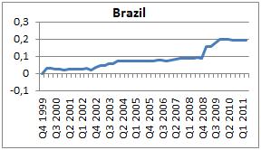
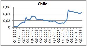
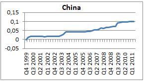
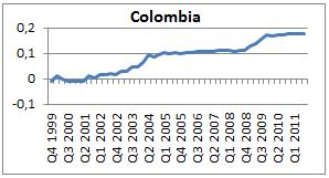
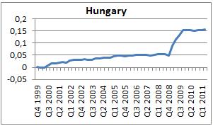
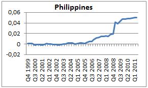
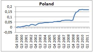
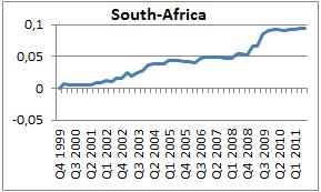
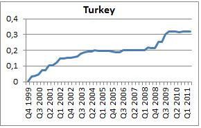
104 Table 5 104

105 Following this we will now turn to the statistical results. These are shown in table 6. First note that as in the univariate analysis we impose restrictions on the coefficients, so they are in line with what the theory predicts. However, as shown by Rapach et. Al. (2010) imposing restrictions on the slope have marginal effect on the forecast. As they notes, this may be due to the fact that CF always satisfies the theoretical restrictions. To limit the scope we have not made comparison forecast in respect to this, but based on Rapach et.al. we would argue that these restrictions have little effect in respect to the CF. As seen from the results in the table below, all the MSE F test statistics are significant. But when it comes to the ENC NEW none prove statistically significant. Thus, the HA benchmark model encompasses the CF for all countries, throughout the OOS sample period. But the MSPE is significantly lower for all the CF compared to HA. This is not common findings, and why this is the case is beyond our technical capabilities to explain. So to get a better fundament to comment on the results we can look at the Sharpe ratios. As seen from the table below, all the Sharpe ratios from the CF are higher than the alternative strategy (buy-and-hold or restricted). Furthermore in 11 of the 20 EM`s the Sharpe ratios are significantly higher when compared using the test developed by Schmid & Schmidt (2007). This could be seen as quite convincing indication that an investor is able to exploit information from these twelve conditional variables to deliver higher abnormal returns. As discussed in chapter 3 one reason why investors should invest in EM are due to the diversification gains. So in most cases a US investor is not just interested in investing in one EM, Thus, a he will in most cases look at the whole EM universe. To see how our models perform from this perspective we have looked at how the CF`s perform in this perspective, and the results are remarkably good. This are presented and discussed in part

106 Table 6 COMBINED ALL ARGENTINA BRAZIL CHILE MSE-F ** MSE-F *** MSE-F ** ENC-NEW ENC-NEW ENC-NEW Sharpe Sharpe Sharpe Test Stat * Test Stat * Test Stat * CHINA COLOMBIA CZECH MSE-F *** MSE-F *** MSE-F *** ENC-NEW ENC-NEW ENC-NEW Sharpe Sharpe Sharpe Test Stat Test Stat ** Test Stat HUNGARY INDIA INDONESIA MSE-F *** MSE-F *** MSE-F *** ENC-NEW ENC-NEW ENC-NEW Sharpe Sharpe Sharpe Test Stat * Test Stat Test Stat * ISRAEL MALAYSIA MEXICO MSE-F *** MSE-F *** MSE-F *** ENC-NEW ENC-NEW ENC-NEW Sharpe Sharpe Sharpe Test Stat * Test Stat ** Test Stat ** PAKISTAN PHILIPPINES POLAND MSE-F *** MSE-F ** MSE-F *** ENC-NEW ENC-NEW ENC-NEW Sharpe Sharpe Sharpe Test Stat Test Stat Test Stat SOUTH-AFRICA SOUTH-KOREA TAIWAN MSE-F *** MSE-F *** MSE-F *** ENC-NEW ENC-NEW ENC-NEW Sharpe Sharpe Sharpe Test Stat ** Test Stat ** Test Stat THAILAND TURKEY MSE-F *** MSE-F *** ENC-NEW ENC-NEW Sharpe Sharpe Test Stat Test Stat

107 8.3 COUNTRY ALLOCATION In this part we will use the predictions from the CF forecasts from each country. The strategy we follow is the same as the one used up to know and explained in chapter 7.1. Thus, we use data from our combined return forecast from model (8.1) denoted by,, and we construct a portfolio consisting of stock or 3 month US Treasury bill, where the latter is by,. If then the investor buys stock and sells the risk free instrument. When the opposite is true, then we short stocks and buy the risk free instrument. This is done through the end of the OOS sample. But in addition we include weights formed by the MSCI. To simplify we use the weights used by MSCI pr These are displayed in appendix 6. As we only have 17 countries of the MSCI index which include 21. We readjust the weights so they sum to 100, these are displayed in the same appendix. The rest of the countries, Argentina, Pakistan and Israel are hence excluded in this analysis. Following this if e.g. our model predicts higher returns than the US TB in Brasil 15,74% for Q then we will put 15,74% of our portfolio in Brazilian stock index, and borrow at US TB. If the returns are lower we will short 15,74% of our portfolio in Brazil and instead put our money in US TB. This will follow from all 17 EM. This strategy will then be compared against the returns from a buy-and-hold strategy. Thus we go long in the MSCI EM index throughout the whole OOS sample period, which as noted spans from Q till Q (or Q3). Note that we compare Sharpe ratios so the returns are risk adjusted. Furthermore the return constructed for the MSCI is not the real MSCI returns, as we use data gathered from different indexes (mostly IFC), the returns from the MSCI are approximated using the same weights as the MSCI EM index uses. We assume the indexes are quite comparable, but it might bias the optimal weights. But as both are gathered from the same source we would argue that it is consistent and will not affect the credibility off our findings. 107

108 As seen from our findings our strategy delivers a considerably higher return compared to just go long in the MSCI EM index. The trading strategy delivers returns of 26.4% compared to the buy-and-hold which deliver 10.8%. When risk adjusted returns are compared, the trading strategy delivers significantly higher Sharpe ratio on almost a 99% significance level (c-value equals 2.42). 22 From a theoretical asset allocation perspective, if expected return is to some extent predictable, then the optimal asset allocation strategy changes from a constant mix (benchmark) to a dynamic investment strategy, where the allocation is conditional on expected return. Our findings prove this to some extent and show that if one combines information from conditional variables into an asset allocation strategy it will enhance risk adjusted returns. Note that, to simplify, we have not included transaction costs in this analysis. It is obvious that the return would have decreased, but as the results show a significant level of 99% it is reasonable to assume that including transaction cost would not have changed the conclusion considerably. Summary In this part we have look at how the conditional variables have performed by utilize the information from all of them into one single forecast for each EM. We follow the procedure recently applied by Rapach et. Al. (2010) which proved to deliver superior OOS gains relative to individual forecasts. Consistently with their findings we find that by combining the individual predictors into a simple average CF we are able to improve the OOS forecasts. However the test statistics gives remarkably contrary results, where the MSE F proves significant for all countries and the ENC-NEW for none. These are not common 22 The results are displayed in appendix

109 findings and are beyond our technical capabilities to comment on. But by further basing interference on the Sharpe ratios all proves to higher and 11significantly higher than the alternative strategy. Furthermore as an investor in most cases is not just interested in one EM, we have looked at how our trading strategy performs investing in all EM combined. This show quite remarkably results where we, by utilizing information through the CF, are able to deliver significantly higher risk adjusted returns compared to a proxy of the MSCI index. 9. CONCLUSION During the last two decades, a great number of markets categorized as less advanced, have made an extensive improvement in their financial structure, where stock market transactions are developing and increasing faster than developed markets. These markets are revealed as emerging. This has opened new investment opportunities and due their low correlation with developed markets, investing in EM can provide increased diversification benefits for a global investor. These and other aspects important to get a fundamental overview of why EM`s are interesting are discussed in chapter 3 and 4. In this context, this thesis aims to examine evidence of stock return predictability in EM`s, and if statistical evidence is found is a US investor able to exploit this to consistently deliver higher abnormal returns. Stock return predictability is arguably without doubt the most intensely debated issue of empirical asset pricing. Over the past 30 years a growing stand of researchers have found evidence for stock return predictability. In chapter 5 we investigate the beginning of predictability of asset returns and seek to give the reader a fundamental overview of return prediction theory. Furthermore, understanding the theories offers information that can be used to develop a good forecasting model, and motivates to choice of conditional variables. 109

110 In traditional capital market theory it is assumed that expected return is constant over time. Later, however research has implied that expected return varies over time and that it has a clear business-cycle pattern. Chen, Roll and Ross (1986), Fama and French (1989) and Chen (1991) argued when business conditions are assiduously poor, agents require a higher premium to stimulate investment in risky assets, where the opposite is case when business conditions are strong. Fama and French (1988) and Balvers er al. (1990) explain this by the use of Life Cycle Permanent Income hypothesis and show that expected return must be time variant, if marginal utility is not constant. This was further extended by Campbell and Cochrane (1999) by including risk aversion to be time variant. The idea that predictability stems from counter cyclical variation in expected return offers motivation to include several different conditional variables. In this thesis we have included macroeconomic-, valuation-, technical and global variables, which in total amount to twelve. These are further explained in chapter 6, where we provide the reader with an in dept theoretical foundation of the different variables used to predict stock returns in EM. In chapter 7 we first present the theoretical framework and discuss potential econometric issues, before the empirical results, of the predictive ability of each twelve conditional are presented. In addition to both IS and OOS testing, we make use of a simple trading strategy to see if the conditional variables are able to provide information which can deliver consistently abnormal returns for a US investor. It was shown that the results are mixed; displaying an uncommon mix of relatively poor IS results, compared to OOS. It is common to find poor forecasting results during the 90`s, so the increased predictability during the OOS forecast period may be due to a drastic change in the EM environment. However based on the Sharpe ratios of the trading strategy, the variables performed quite poorly. Overall due to the fact that some variables are quite persistent and not fulfill the normality assumption, results have to be taken with care. In the last part we first look at how the conditional variables have performed by utilize the information from all of them into one single forecast for each EM. We follow the procedure recently applied by Rapach et al (2010) which proved to deliver superior OOS gains relative to individual forecasts. Consistently with their findings we find that by combining 110

111 the individual predictors into a simple average CF we are able to improve the OOS forecasts. However the test statistics gives remarkably contrary results, where the MSE F proves significant for all countries and the ENC-NEW for none. By further basing interference on the Sharpe ratios all proves to higher and 11significantly higher than the alternative strategy. Furthermore as an investor in most cases is not just interested in one EM, we have looked at how our trading strategy performs investing in all EM combined. This show quite remarkably results where we, by utilizing information through the CF, are able to deliver significantly higher risk adjusted returns compared to a proxy of the MSCI index. Overall we have found that by combining individual forecast, a US investor is able to consistently deliver abnormal returns. However whether this persists in the future is obviously hard to say. But despite a number of limitations, and some arbitrary decisions, this paper has addressed an important topic and makes a contribution to the existing literature by investigating some of the most recent developments within the field of empirical asset pricing. 111

112 REFERENCE LIST SCIENTIFIC PAPERS K. Geert Rouwenhorst (1999). Local Return Factors and Turnover in Emerging Stock Markets. The Journal of Finance, Vol. Liv, No. 4. J.Y. Campbell & J.H. Cochrane (2000). Explaining the poor performance of consumption-based asset pricing models. The Journal of Finance, Vol. Lv, No. 6. S. Michelson, E. Philipova & P. Srotova (2008). The Case For Emerging Market Funds. Journal of Business & Economic Research, Vol 6, Nr. 11 G. Bekaert & C. R. Harvey (2002). Research in emerging markets finance: looking to the future. Emerging Markets Review 3(2002) pp C.J. Neely, D. E. Rapach, J. Tu & Guofu Zhou (2010). Out-of-Sample Equity Premium Prediction: Fundamental vs. Technical Analysis. Unpublished working paper, Washington University in St. Louis H. Guo (2006). Out-of-Sample Predictability of Stock Market Returns. The Journal of Business, Vol. 79, No. 2 pp J.D. Hamilton (1989). A New Approach to the Economic Analysis of Nonstationary Time Series and the Business Cycle. The Economic Society, Vol. 57, No 2, pp R.J. Balvers, T.F. Cosimano & B. McDonald (1990). Predicting stock return in an efficient market. The Journal of Finance, Vol. 45, No. 4, pp J. Conrad & G. Kaul (1988). Time-variation in Expected Returns. The Journal of Business, Vol. 61, No. 4, pp T. Chordia & L. Shivakumar (2002). Momentum, Business Cycle and Time-Varying Expected Returns. The Journal of Finance, Vol. 57, No. 2, pp T. Sener & P.B Girma (2010). Sources Of Variability In Global Equity Returns. International Business & Economic Research Journal, Vol. 9, No. 9 A. Mele (2007). Asymmetric stock market volatility and the cyclical behavior of expected returns. Journal of Financial Economics, No. 86, pp R. Haselman (2010). Foreign banks and financial stability in emerging markets: Evidence from the global financial crisis. CEPR and Bank of Finland, Helsinki. J. Estrada (2000). The Cost Of Equity In Emerging Markets: A Downside Risk Approach. Department of Finance, Emerging Markets Quarterly, 4. A.P. Serra (2000). Country and Industry Factors in Returns: Evidence From Emerging Markets Stocks. Emerging Markets Review 1, pp D.A. Glassman & L.A. Riddick (1989). A Generalized Model Of International Portfolio Diversification: Evaluating Alternative Specifications. UCLA Working Paper 565 G. Bekaert & C.R. Harvey (1994). Time-Varying World Market Integration. Working Paper No S.G. Cecchetti, P. Lam & N.C. Mark (1988). Mean Reversion In Equilibrium Asset Prices. Working Paper No J.B. de Macedo, J.A. Goldstein & D.M Meerschwam (1982). International Portfolio Diversification: Shortterm Financial Assets and Gold. National Bureau Of Economic Research. Working paper No S.J. Khoury (2003). Country Risk and International Portfolio Diversification for the Individual Investor. Financial Services Review No. 12 pp S.R. Das & R. Uppal (2004). Systemic Risk and International Portfolio Choice. The Journal Of Finance, Vol. Lix, No

113 P. Giot & M. Petitjean (2011). On the Statistical and Economic Performance of Stock Return Predictive Regression Models: An International Perspective. Quantitative Finance, Vol. 11, No.2, pp A. Marathe & H.A. Shawky (1994). Predictability of Stock Returns and Real Output. The Quarterly Review of Economics and Finance, Vol. 34, No. 4, pp A. Timmermann & C.W.J. Granger (2004). Efficient Market Hypothesis and Forecasting. International Journal of Forcasting, 20, pp R. Morck, B. Yeung & W. Yu (2000). The Information Content of Stock Markets: Why Do Emerging Markets have synchronous Stock Price Movements? Journal of Financial Economics, 58, pp J. Estrada (2002). Systematic Risk in Emerging Markets: The D-CAPM. Emerging Markets Review, 3, pp J.Y Campbell & C. Polk (2010). Growth or Glamour? Fundamentals and Systematic Risk in Stock Returns. The Review of Financial Studies /v 23 No. 1. D.E. Rapach & M.E Wohar (2005). In-Sample vs. Out-of-Sample tests of Stock Return Predictability in the Context of Data Mining. Journal of Empirical Finance (2006) Volume: 13, Issue: 2, Pages: Neely, C.J., Rapach, D.E., Tu, J., Zhou, G. (2011). Forecasting the equity risk premium: the role of technical indicators. Federal Reserve Bank of St. Louis Working Paper C. D.E. Rapach, J.K. Strauss & G. Zhou (2009). Out-of-Sample Equity Premium Prediction: Combination Forecasts and Links to the Real Economy. The Review of Financial Studies /v 23, No. 2 D. Pettenuzzo & A. Timmermann (2011). Predictability of Stock Returns and Asset Allocation Under Structural Breaks. Journal of Econometrics. 2011, 164, C.M Bilson, T.J. Brailsford & V.J. Hooper (2001). Selecting Macroeconomic Variables as Explanatory Factors Of Emerging Stock Market Returns. Pacific-Basin Finance Journal, 9, pp A. Schrimpf (2010). International Stock Return Predictability Under Model Uncertainty. Journal of International Money and Finance, 29, pp YL. Cheung & YK. Ho. (1991). The Intertemporal Stability of the Relationships between the Asian Emerging Equity Markets and the Developed Equity Markets. Journal of Business Finance & Accounting, 18(2). I. Welch & A. Goyal (2008). A Comprehensive Look at the Empirical Performance of Equity Premium Prediction. The Review of Financial Studies /v 21, No. 4. W.E. Ferson & C.R. Harvey (1998). Fundamental Determinants of National Equity Market Returns: A Perspective on Conditional Asset Pricing. Journal of Banking & Finance, 21, pp L.Bonga-Bonga & M. Makakabule (2010). Modeling Stock Returns in the South African Stock Exchange: A Nonlinear Approach. European Journal of Economics, Finance and Administrative Sciences, Issue 19. K. Mio (2010). Quantitative Analysis of the Growth Potential and Resilience of Emerging Markets in the G-20. NLI Research. G. De Santis & B. Gerard (1995). Time-Varying and International Portfolio Diversification with Contagious Bear Markets. Institution for Empirical Macroeconomics. Discussion paper 99. M.L. Matika (2009). South Africa Aspirant Multinationals and their Move into Emerging Market Economies: How Emerging Markets are Chosen for Market Entry: Standard Bank as a Case Study. Gordon Institute of Business Science. G. Bekaert, C.R. Harvey &R.L. Lumsdaine (2002) "The dynamics of emerging market equity flows." Journal of International Money and Finance, Elsevier, vol. 21(3), pp D.E. Rapach, M.E. Wohar (2006) In-sample vs. out-of-sample tests of stock return predictability in the context of data mining, Journal of Empirical Finance vol. 13, pp T.E. Clark, M.W. McCracken (2001). Tests of Equal Forecast Accuracy and Encompassing for Nested Models, Journal of Econometrics 105, pp

114 M.W. McCracken (2007), Asymptotics for Out of Sample Tests of Granger Causality, Journal of Econometrics 140, pp M. Guidolin, C. Fangzhou Na (2006), The Economic and Statistical Value of Forecast Combinations under Regime Switching: An Application to Predictable US Returns, Research Division: Federal Reserve Bank of St. Louis Working paper series B G. Bakshi(a), G. Panayotov(b), G. Skoulakis(c) (2011), The Baltic Dry Index as a Predictor of Global Stock Returns, Commodity returns, and Global Economic Activity, (a) Smith School of Business, University of Maryland, (b) McDonough School of Business, Georgetown University, (c) Smith School of Business, University of Maryland - Working Paper Series I. Bunda, A. J. Hamann, S. Lall (2005), Comovement in Emerging Market Bond Returns: An Empirical Assessment, Laboratoire d`economie d`orleans Working Paper. S.F. LeRoy (1989); Efficient Capital Markets and Martingales; Journal of Economic Literature 1989, Vol. 27, No. 4 R. Gupta, M.P Modise (2011), Macroeconomic Variables and South-African Stock Return Predictability ; Department of Economics, Working Paper Series T. Bollerslev, G. Tauchen, H. Zhou (2009); Expected Stock Returns and Variance Risk Premia ; Oxford Journals Advance Access publication, Feb. 12, T. Sener, P.B. Girma (2010); Source Of Variability In Global Equity Returns, International Business & Economics Research Journal Sep. 2010, Vol. 9, nr. 9. T. Bollerslev, J. Marrone, L. Xu, H. Zhou (2011); Predicting Stock Returns with Variance Risk Premia: Statistical Interference and International Evidence, Division of Research and Statistics, Federal Reserve Board Washington. A.ang, G. Bekaert (2006), Stock Return Predictability: Is it There?, Oxford Journals, Advance Access publication July J. H. Stock, M. W. Watson (2003); Combination Forcasts Of Output Growth In A Seven-Country Data Set, Department of Economics, Harvard University. C. Calderon, R. Fuentes (2010); Characterizing the Business Cycles of Emerging Economies, Policy Research Working Paper 534, The World Bank. M. Sanchez (2007), What Dives Business Cycles And International Trade In Emerging Market Economies?, European Central Bank Working Paper Series NO 730 / February C. Bilson, T. Brailsford, V. Hooper (1999); Selecting Macroeconomic Variables As Explanatory Factors Of Emerging Stock Market Returns, Department of Commerce, Australian National University. P. Bossaerts, P. Hillion (1999); Implementing Statistical Criteria to Select Return Forecasting Models: What Do We Learn?, The Review of financial Studies, Vol. 12, No. 2, pp M. Aguiar, G. Gopinath (2007); Emerging Market Business Cycles: The Cycle Is the Trend, Journal af Political Economy, 2007, vol. 115, no. 1. J. Y. Campbell, S. B. Thompson (2004/2007); Predicting Excess Stock Returns Out of Sample: Can Anything Beat the Historical Average?, Department of Economics, Harvard University. J.Y. Campbell, M. Yogo (2006); Efficient Tests Of Stock Return Predictability, Journal of Financial Economics 81, 2006, H.J. Chen, H. Ortiz-Molina, S.S. Zhang (2010); Average Stock Variance and Market Returns: Evidence of Time-varying Predictability at the Daily Frequency, Sauder School of Business, University of British Colombia. M. Kortas, J.F. L`Her, M. Roberge (2005); Country Selection of Emerging Equity Markets: Benefits from Country Attribute Diversification, Emerging Markets Review 6, 2005, pp J. N. Erisken, K. H. Mikkelsen (2010); Forudsigelse af aktiemarkedet: En in-sample og out-of-sample undersøgelse af det aggregerende danske aktiemarked, Handelshøyskolen i Århus. 114

115 L.M.C.S Menike (2006); The Effect of Macroeconomic Variables on Stock Prices in Emerging Sri Lankan Stock Market, Sabaragamuwa University Journal, vol. 6, no. 1, pp S.G.M Fifield, D.M. Power, C.D. Sinclair (2002); Macroeconomic Factors And Share returns: An Analysis Using Emering Market Data, International Journal of Finance and Economics, no.7,pp A. Timmermann (2005); Forecast Combinations, USCD, Aug. 27, 2005 W. E. Ferson, C.R. Harvey (1998); Fundamental Determinants of National Equity Market Returns: A Perspective on Conditional Asset Pricing, Journal of Banking & Finance, 21, pp W.E. Ferson, C.R. Harvey (1998); Fundamental Determinants Of National Equity Market Returns: A perspective on Conditional Asset Pricing, Journal of Banking & Finance, 21, pp I. Welch, A. Goyal (2007); A Comprehensive Look at The Empirical Performance of Equity Premium Prediction, Oxford Journals, Advance Access Publication, March 17, M. Dahlquist, C.R. Harvey (2001); Global Tactical Asset Allocation, Centre for Economic Policy Research, London. M. Lettau, S.C. Ludvigson (2010); Marketing and Modeling Variation in the Risk Return trade off, Department of Economics, NY, Chapter 11. W.E. Ferson, C.R. Harvey (1994/1996); Fundamental Determinants of National Equity Market Returns: A Perspective on conditional Asset Pricing, Finance of the Department of Finance and Business Economics. G. Bekaert, X. Wang (2010); Inflation Risk, Economic Policy, October A. Inoue, L. Kilian (2002); In-Sample or Out-Of-Sample Tests of Predictability: Which One Should We Use?, European Central Bank - Working Paper No. 195, Nov P. Giot, M. Petitjean (2006); International Stock Return Predictability: Statistical Evidence and Economic Significance, CORE Discussion Paper 2006/88. D.E. Rapach, M.E. Wohar (2002); In-Sample vs. Out-Of-Sample Tests of Stock Return Predictability in the Context of Data Mining, Departments of Economics, Seattle University & University of Nebraska. W.E.Ferson, S. Sarkissian, T. T. Simin (2003); Spurious Regressions in Financial Economics, the Journal of Finance, Vol. LVIII, No. 4, August M.Lettau, S. Ludvigson (2001); Consumption, Aggregate Wealth, and Expected Stock Returns, Journal of Finance, Vol. LVI, No. 3, June J. Lewellen (2004); Predicting Returns with Financial Ratios, Journal of Financial Economics 74, pp C.J. Neely, D.E. Rapach, J.Tu, G. Zhou (2010); Forecasting the Equity Risk Premium: The Role of Technical Indicators, Federal Reserve Bank of St. Louis Working Paper Series. A. Harri, B.W. Brorsen (2009); The Overlapping Data Problem, Quantitative and Qualitative Analysis in Social Sciences, Vol. 3, Issue 3, 2009, pp C. Park (2006); The Persistence and Predictive Power of the Dividend-Price Ratio, Departments of Economics Working Paper No D. Pettenuzzo, A. Timmermann (2011); Predictability of Stock Returns and Asset Allocation Under Structural Breaks, Journal of Econometrics, doi: /j D.E Rapach, M.E Wohar (2003); Valuation Ratios and Lon-Horizon Stock Price Predictability, Department of Econometrics, Oct. 23, 2003 D.E. Rapach, M.E. Wohar, J. Rangvid (2004); Macro Variables and International Stock Return Predictability, International Journal of Forecasting, forthcoming, May 7, D.E. Rapach, J.K Strauss, G. Zhou (2009); Out-Of-Sample Equity Premium Prediction: Combination Forecasts and Links to the Real Economy, Oxford Journals, Advance Access Publication, Aug. 11, D.E. Rapach, M.E. Wohar (2006); Structural Breaks and Predictive Regression Models of Aggregate U.S Stock Returns, Department of Economics, Jan. 19, 2006 (Revised). 115

116 J.H.Stock, M.W. Watson (2003); How Did Leading Indicator Forecasts Do During The 2001 Regression, Departments of Economics, Harvard University & Princeton University. A.P. Serra (2002); The Cross-Sectional Determinants or Returns Evidence from Emerging Markets Stocks,Investigação - Trabalhos em curso - nº 120, Outubro de 2002 Working Papers Da FEP. R. Gupta (2011); Macroeconomic Variables and South African Stock Return Predictability, Department of Economics Working Paper Series University of Pretoria. P. Giot, M. Petitjean (2009) On the Statistical and Economic Performance of Stock Return Predictive Regression models: An International Perspective, Quantitative Finance, Vol. 11, No. 2, pp E.F. Fama (1970). "Efficient Capital Markets: A Review of Theory and Empirical Work". Journal of Finance 25 (2): J. Y. Campbell, A. W. Lo, A. C. MacKinlay (1997); The Econometrics of Financial Markets; Princeton University Press 1997 W.F.M. DeBondt, R. Thaler (1985); Does The Stock Market Overreact?, Journal Of Finance, Vol. 40, Issue 3, July 1985, pp J. C.M., G. Kaul (1996). Oil and the Stock Market, Journal of Finance, 51, W. E. Ferson & C. R. Harvey (1991); The Variation of Economic Risk Premiums; Journal of Political Economy, Vol. 99, 1991 Nai-Fu Chen, Richard Roll, Stephen A. Ross (1986); Economic Forces and the Stock Market; The Journal of Business, Vol. 59, No. 3, 1986 F. E. Fama and Kenneth R. French, 1988, Permanent and temporary components of stock prices, Journal of Political Economy 96, Pesaran, M. H. and Timmermann, A., A simple non-parametric test of predictive performance. Journal of Business and Economic Statistics; 10(4): J. Lakonishok, A. Schleifer, R.W. Vishny (1994); Contrarian Investment, Extrapolation and Risk, Journal Of Finance, 1994 Helmut Reisen (2000) Pensions, Savings and Capital Flows, 2000, 277 pp Barry, I I I Peavy, M Rodriguez in Financial Analysts Journal (1998) Performance Characteristics of Emerging Capital Markets Goetzmann, William N. & Rouwenhorst, K. Geert (ed.), "The Origins of Value: The Financial Innovations that Created Modern Capital Markets," OUP Catalogue, Oxford University Press, number , October Richard C. Grinold, Ronald N. Kahn McGraw-Hill Professional, Business & Economics pages Martijn Cremers; (2002); Stock Return Predictability: A Bayesian Model Selection Perspective Review of Financial Studies, Vol. 15, No. 4, Pp , 2002 E. F. FAMA (1991); Efficient Capital Markets: II THE JOURNAL OF FINANCE.VOL. XLVI, NO. 5 DECEMBER 1991, Journal of Financial Economics, Vol. 6, Nos. 2/3, pp , 1978 Summers, LawrenceH., 1986, Does the stock market rationally reflect fundamental values?, Journal of Finance 41, Rapach, D. E., J. K. Strauss, and G. Zhou Out-of-Sample Equity Premium Prediction: Combination Forecasts and Links to the Real Economy.Review of Financial Studies 23: Hodrick(1992) standard errors: "Dividend Yields and Expected Stock Returns: Alternative Procedures for Inference and Measurement", Review of Financial Studies, vol 5, no 3, Campbell, John Y. and Samuel B. Thompson Predicting excess stock returns out of sample: Can anything beat the historical average? The Review of Financial Studies 21(4): Reinhart, Carmen & Reinhart, Vincent, "Diminished Expectations, Double Dips, and External Shocks: The Decade After the Fall," MPRA Paper 24969, University Library of Munich, Germany. 116

117 R. Ackerman (2010); Charitable Giving Continues Despite Economic Stress ; Financial Planning, July 9, 2010 Y. Tokat and N. W. Wicas (2004); International Equity Investing: Investing in Emerging Markets, Journal of Wealth Management 6(2) pp.68-80, Published in Vanguard. Bekaert, Geert & Harvey, Campbell & Lundblad, Christian T., "Liquidity and Expected Returns: Lessons from Emerging Markets," CEPR Discussion Papers 5946, C.E.P.R. Discussion Papers Elton, Gruber, Brown, Goetzmann(2007): Modern Portfolio Theory and Investment Analysis, 6th Edition A.B. Divecha, J. Drach, D. Stefek (1992); Emerging Markets: A quantitative perspective, The Journal of Portfolio, Fall 1992, Vol 19, No. 1, pp William N. Goetzmann & Lingfeng Li & K. Geert Rouwenhorst, "Long-Term Global Market Correlations," The Journal of Business, University of Chicago Press, vol. 78(1), pages 1-38 Sharpe, W.F., Capital Asset Prices: A Theory of Market Equilibrium under Conditions of Risk, Journal of Finance 19, Lintner, J., The valuation of risk assets and selection of risky investments in stock portfolios and capital budgets, Review of Economics and Statistics 47, C. R. Belfield (1999); The Behaviour of Graduates in the SME Labour Market: Evidence and Perceptions, Volume 12, Number 3. P.L. Bernstein, A. Damodaran (1998) Portfolio management; Investment analysis, Publisher J.Wiley (New York) Summers, Lawrence H., 1986, Does the stock market rationally reflect fundamental values?, Journal of Finance 41, Shiller, R. J. (1984): Stock Prices and Social Dynamics, Brookings Papers on Economic Activity, 2, G. B. Malkiels (1973) A Random Walk Down Wall Street. Samuelson, P.A. 1965, Proof That Properly Anticipated Prices Fluctuate Randomly, Industrual Management Review, vol. 6, nr. 2, pp Mehra, Rajnish; Edward C. Prescott (1985). "The Equity Premium: A Puzzle" (PDF). Journal of Monetary Economics 15 (2): Ronald J. Balvers, Thomas F. Cosimano, Bill McDonald. Predicting Stock Returns in an Efficient Market Journal of Finance, Volume 45, Issue 4 (Sep., 1990), James M. Poterba, Lawrence H. Summers (1987); The Persistence of Volatility and Stock Market Fluctuations NBER Working Paper No LeRoy, S., Risk Aversion and the Martingale Property of Stock Prices, International Economic Review, 14, CHEN, N, ROLL, R. and ROSS, S. (1986) Economic Forces and the Stock Market, Journal of Business. Vol 59, No 3, pp Modigliani, F. and R. Brumberg (1955) Utility Analysis and the Consumption Function: An Interpretation of Cross-Section Data, in K. K.Kurihara (ed.), Post-Keynesian Economics, New Brunswick, NJ: Rutgers University Press. John Y. Campbell & John Cochrane, "Force of Habit: A Consumption-Based Explanation of Aggregate Stock Market Behavior," Journal of Political Economy, University of Chicago Press, vol. 107(2), pages Stephen F. LeRoy (1989); Efficient Capital Markets and Martingales, Journal of Economic Literature, Vol. 27, No. 4. (Dec., 1989), pp Sims, Christopher A., Stickiness, Carnegie-Rochester Conference Series on Public Policy 49: (1998). 117

118 Sims, Christopher A., Implications of Rational Inattention, Journal of Monetary Economics 50: (2003). David A. Hirshleifer (2001); Investor Psychology and Asset Pricing, University of California, Irvine - Paul Merage School of Business. A. P. Serra (2000) The Cross-Sectional Determinants of Returns: Evidence from Emerging Markets' Stocks, Faculdade de Economica do Porto, Universidade do Port Bekaert,G.,Hodrick,R.J.,Marshall,D.,1997a.Onbiasesintestsoftheexpectationshypothesisof the term structure of interest rates. Journal of Financial Economics 44, Bekaert, G., Hodrick, R.J., Marshall, D., 1997b. The implications of first-order risk aversion for asset market risk premiums. Journal of Monetary Economics 40, Kargin, Vladislav, "Value investing in emerging markets: risks and benefits," Emerging Markets Review, Elsevier, vol. 3(3), pages , September Fama, Eugene F. & French, Kenneth R., "Business conditions and expected returns on stocks and bonds," Journal of Financial Economics, Elsevier, vol. 25(1), pages 23-49, November Michael S. Rozeff (1984); Dividend Yields Are Equity Risk Premiums Journal of Portfolio Management, pp , Fall 1984 John Y. Campbell and Robert J. Shiller (2001); Valuation Ratios and the Long-Run Stock Market Outlook: An Update, Cowles Foundation for Research In Economics Yale University, Cowles Foundation, Discussion Paper No Campbell, John Y. and Robert J. Shiller (1988a), "The Dividend-Price Ratio and Expectations of Future Dividends and Discount Factors", Review of Financial Studies 1: , Fall Rangvid, J. (2006). Output and Expected Returns. Journal of Financial Economics, 81, Fama, E.F. and French, K. (1998b) Value versus growth: the international evidence. Journal of Finance 53(6), Martin Lettau & Sydney Ludvigson, "Expected Returns and Expected Dividend Growth," NBER Working Papers 9605, National Bureau of Economic Research, Inc W. Beaver, D. Morse (1978); What Determines Earnings Price Ratios?, Financial Analyst Journal (July/August 1978), Nathan S. Balke & Mark E. Wohar, "Low frequency movements in stock prices: a state space decomposition," Working Papers 00-01, Federal Reserve Bank of Dallas J.A. Ou, S.H. Penman (1989); Financial Statement Analysis and the Prediction of Stock Returns, Journal of Accounting and Economic 11. Berk, J., A critique of size related anomalies. Review of Financial Studies 8, Sharathchandra,G.,Thompson,R.,1994. Book-to-market as a surrogate for priced risk when risk is time varying. Working paper. Southern Methodist University, Dallas, TX. J. Pontiff, and L. Schall. Book-to-market ratios as predictors of market returns. Journal of Financial Economics.1998, 49: Flannery, M., Protopapadakis, A., Macroeconomic factors do influence aggregate stock returns. Review of Financial Studies 15, Harvey, C.R. (1988), The Real Term Structure and Consumption Growth, Journal of Financial Economics 22, Fama, Eugene F. & French, Kenneth R., "Business conditions and expected returns on stocks and bonds," Journal of Financial Economics, Elsevier, vol. 25(1), pages N. Chen (1991); Financial Investment Opportunities and the Macroeconomy, Journal of Finance, 1991, vol. 46, issue 2, pages Christopher Polk, Samuel Thompson & Tuomo Vuolteenaho (2006); Cross Section Forecasts of the EquityPremium; Journal of Financial Economics, Vol. 81, No. 1,

119 Rapach, D.E., Wohar, M.E., & Rangvid, J. (2005). Macro variables and international stock return predictability. International Journal of Forecasting, 21: Fisher, Irving. The Rate of Interest. New York: MacMillan Company, Fama E (1975), Short Term Interest Rates as Predictors of Inflation, American Economic Review, 65, June, Hamilton, James D., 1985, Uncovering financial market expectations of inflation, Journal of Political Economy 93, Andrew Ang & Geert Bekaert & Min Wei, "The Term Structure of Real Rates and Expected Inflation," Journal of Finance, American Finance Association, vol. 63(2), pages , 04 Frederic S. Mishkin, "What Does the Term Structure Tell Us About Future Inflation?," NBER Working Papers 2626, National Bureau of Economic Research, Inc King, Robert G., James H. Stock, and Mark W. Watson Temporal Instability of the Unemployment- Inflation Relationship. Economic Perspectives of the Federal Reserve Bank of Chicago, May-June, Estrella, Arturo & Hardouvelis, Gikas A, " The Term Structure as a Predictor of Real Economic Activity," Journal of Finance, American Finance Association, vol. 46(2), pages , June Fama, E. F. (1981), Stock Returns, real Activity, Inflation, and Money, American Economic Review, 71 Geske, R., and R. Roll, The Monetary and Fiscal Linkage between Stock Returns and Inflation, Journal of Finance, 38 Brandt, M., and K. Wang (2003): Time-Varying Risk Aversion and Unexpected Inflation, Journal of Monetary Economics, 50, Steven A. Sharpe, "Reexamining Stock Valuation and Inflation: The Implications Of Analysts' Earnings Forecasts," The Review of Economics and Statistics, MIT Press, vol. 84(4), pages Yin Wu, Stock Prices and Exchange Rates in A VEC Model-The Case of Singapore in the 1990s, Journal of Economics and Finance, Volume 24, Number 3, Pages Kausik Chaudhuri & Yangru Wu, "Random Walk versus Breaking Trend in Stock Prices: Evidence from Emerging Markets," Working Papers , University of Sydney, Department of Economics Demir, O., Demirhan, E., The relationship between stock prices and exchange rates: Evidence from Turkey, International Research Journal of Finance and Economics, Issue 23, pp Cochrane, John, "Financial Markets and the Real Economy", NBER Working Papers No Cooper, I., and R. Priestley, 2009, Time-Varying Risk Premiums and the Output Gap, Review of Financial Studies, 22(7), July, Fuhrer,J.,andG.Rudebusch(2004): Estimating the Euler Equation for Output, Journal of Monetary Economics, 51(6), Clarida,R.,J.Gali, andm.gertler(2000): Monetary Policy Rules and Macroeconomic Stability: Evidence and Some Theory, Quarterly Journal of Economics, 115, Fama. Eugene F. and Kenneth R. French, 1988, Permanent and temporary components of stock prices, Journal of Political Economy 96, J.M Poterba, L.H. Summers (1988); Mean Reversion in Stock Prices: Evidence and Implications, Journal of Financial Economics, 22, Jegadeesh, N., and S. Titman, 1993, Returns to buying winners and selling losers: Implications for stock market efficiency, Journal of Finance, 48, pp Barberis, Nicholas, Andrei Shleifer, and Robert W. Vishny, 1998, A model of investor sentiment, Journal of Financial Economics 49, Daniel, Kent D., David Hirshleifer and Avanidhar Subrahmanyam, 1998, Investor psychology and security market under- and over-reactions, Journal of Finance 53, Hong, Harrison and Jeremy C. Stein, 1999, A unified theory of underreaction, momentum trading and overreaction in asset markets, Journal of Finance 54,

120 Conrad, J., and Kaul, G., 1998, An anatomy of trading strategies, Review of Financial Studies, 11, pp Ronald Balvers & Yangru Wu & Erik Gilliland, "Mean Reversion across National Stock Markets and Parametric Contrarian Investment Strategies," Journal of Finance, American Finance Association, vol. 55(2), pages , Chaudhuri, Kausik, Y. Wu (2004); Mean Reversion in Stock Prices: Evidence from Emerging Markets, Managerial Finance, 30(11), 80 Karolyi, G. A. (2001) Why Stock Return Volatility Really Matters, Preliminary and Incomplete version, February 2001 Pindyck R. (1984) Risk, Inflation and the Stock Market, American Economic Review, 74, pp V. Corradi, W. Distaso and A. Mele, Macroeconomic Determinants of Stock Market Volatility and Volatility Risk Premiums, Updated, September 2011 Corradi, V., W. Distaso, and A. Mele (2009). Macroeconomic Determinants of Stock Market Returns, Volatility and Volatility Risk-Premia. Working Paper. Tim Bollerslev, James Marrone, Lai Xu, Hao Zhou (2011); Stock Return Predictability and Variance Risk Premia: Statistical Inference and International Evidence Working Paper Series, Oct. 11, 2011 Martin Stopford's (2009); Maritime Economics, London: Routledge, Moller, S., Rangvid, J., The fourth-quarter consumption growth rate: A pure-macro, not-estimated stock return predictor that works in-sample and out-of-sample. Working paper. Copenhagen Business School. Michael C. Jense; Some Anomalous Evidence Regarding Market Efficiency Journal of Financial Economics, Vol. 6, Nos. 2/3 (1978). Stock J.H. and M.W. Watson (2004). "Forecasting with many predictors", survey prepared for theforthcoming Handbook of Economic Forecasting. John Y. Campbell, Robert J. Shiller, "The Dividend-Price Ratio and Expectations of Future Dividends and Discount Factors," Review of Financial Studies, Oxford University Press for Society for Financial Studies, vol. 1(3), pages Rapach, D., Strauss, J., and Zhou, G. Out-of-Sample Equity Premium Prediction: Combination Forecasts and Links to the Real Economy. Review of Financial Studies, Vol. 23, No. 2 (2010), pp Todd E. Clark & Michael W. McCracken, "Improving forecast accuracy by combining recursive and rolling forecasts," Research Working Paper RWP 04-10, Federal Reserve Bank of Kansas City Todd E. Clark & Michael W. McCracken, "Tests of Equal Forecast Accuracy and Encompassing for Nested Models," Econometric Society World Congress 2000 Contributed Papers 0319, Econometric Society Ivo Welch & Amit Goyal, "A Note On 'Predicting Returns With Financial Ratios'," Yale School of Management Working Papers amz2465, Yale School of Management. J.M. Bates, C.W.J. Granger (1969); The Combination of Forecast, Operations Research Quarterly, 20, 1969, F.X. Diebold (1989); Forecast Combination and encompassing, reconciling two divergent literatures, International Journal of Forecasting, 5, 1989, pp Hendry, David F & Michael P. Clements, "Economic Forecasting: Some Lessons from Recent Research," Royal Economic Society Annual Conference , Royal Economic Society Friedrich Schmid1and Rafael Schmidt (2007); Multivariate Conditional Versions of Spearman s Rho and Related Measures of Tail Dependence, The Journal of Multivariate Analysis, 98, Elsevier, Robert F. Stambaugh, "Predictive Regressions," NBER Technical Working Papers 0240, National Bureau of Economic Research, Inc. 120

121 Lars Peter Hansen og Robert Hodrick (1980) "Forward Exchange-Rates As Optimal Predictors of Future Spot Rates - An Econometric-Analysis." Journal of Political Economy 88: Newey, Whitney K & West, Kenneth D, "A Simple, Positive Semi-definite, Heteroskedasticity and Autocorrelation Consistent Covariance Matrix," Econometrica, Econometric Society, vol. 55(3), pages , May. Torous, Walter, and Rossen Valkanov, 2000, Boundaries of predictability: Noisy predictive regressions, working paper, UCLA. P.H. Franses & D. Fok & D. van Dijk, "A Multi-Level Panel Smooth Transition Autoregression for US Sectoral Production," Econometric Society 2004 Australasian Meetings 267, Econometric Society Lettau,M.,and S.Van Nieuwerburgh (2007) Reconciling the Return Predictability Evidence: In-Sample Forecasts,Out-of-Sample Forecasts,and Parameter Instability, Review of Financial Studies,21(4), Lettau, M., S. C. Ludvigson, and J. A.Wachter (2008) The Declining Equity Premium: What Role Does Macroeconomic Risk Play?, Review of Financial Studies,21(4), Fama, Eugene F. & French, Kenneth R., (1988). "Dividend yields and expected stock returns," Journal of Financial Economics, Elsevier, vol. 22(1), pages 3-25, October. Fama, Eugene F. and Kenneth R. French, (1988a), Permanent and temporary components of stock prices, Journal of Political Economy 96, Pagan, A.R., "Simulation Based Estimation of Some Factor Models in Econometrics," Department of Economics - Working Papers Series 521, The University of Melbourne Kwiatkowski, D., P.C.B. Phillips, P. Schmidt, Y. Shin (1992): Testing the Null Hypothesis of Stationarity against the Alternative of a Unit Root, Journal of Econometrics, 54, pp , North-Holland. Foster, F. Douglas,Tom Smith, and Robert E.Whaley, 1997, Assessing goodness-of- t of asset pricing models: The distribution of the maximal R-squared, Journal of Finance 52, 591^607. Stambaugh, Robert F., 1986, Bias in Regressions with Lagged Stochastic Regressors, CRSP Working Paper, University of Chicago. Huang, H., and T.-H. Lee To Combine Forecasts or To Combine Information. Econometric Reviews, forthcoming. Clements, M. P., and Harvey, D. I. (2004). Forecast encompassing tests and probability forecasts. Working paper, Department of Economics, University of Warwick. David G. McMillan & Mark E. Wohar, "Stock return predictability and dividend-price ratio: a nonlinear approach," International Journal of Finance & Economics, John Wiley & Sons, Ltd., vol. 15(4), pages BOOKS Timmermann, Allan, "Forecast Combinations," Handbook of Economic Forecasting, C. Sutcliffe (1997); Stock Index Futures, Second Edition. Gujarati, D.N Basic econometrics (4th ed.). Singapore: McGraw Hill. David E. Rapach; Mark E. Wohar; Hamid Beladi (2010); Forecasting in the Presence of Structural Breaks and Model Uncertainty, Frontiers of Economic and Globalization, Vol 3, Emerald Group Publishing Limited, 2010 M. Lettau & S.C Ludvigson (2010). Measuring and Modeling Variation in the Risk-Return trade-off. Handbook of Financial Econometrics 121

122 Aguiar and Gopinath (2007); Emerging Market Business Cycles: The Cycle Is the Trend, Handbook of macroeconomics, Volume 1, part 3 Michael Woodford Gordon, Myron J. (1962). The Investment, Financing, and Valuation of the Corporation. Homewood, IL: R. D. Irwin PAPERS OF RELEVANCE W.L. Megginson & M.K. Boutchkova (2000). The Impact of Privatization on Capital Market Development and Individual Share Ownership. Boutchkova, M.K. and Megginson W.L. (2000), Privatization and the Rise of Global Capital Markets, Financial Management, 29, B. Gerard, P. Hillion, F. de Roon & E. Eiling (2007). International Portfolio Diversification: Currency, Industry and Country Effects Revisited R.G. Clarke, H. de Silva & R. Murdock (2005). A Factor Approach to Asset Allocation: Exposure to global market factors. S. Ranjan Das & R. Uppal (2001). Systemic Risk and International Portfolio Choice. G. A. Karolyi (2003). The Role of ADRs in the Development of Emerging Equity Markets J. Estrada, M. Kritzman & S. Page (2006). Countries Versus Industries in Emerging Markets: A Normative Portfolio Approach. M. Wackernagel (2001). Advancing Sustainable Resource Management: Using Ecological Footprint Analysis for Problem Formulation, Policy Development, and Communication. Standard & Poor`s (2007). S&P Emerging Markets Index: Index Methodology. B. Stine (1998). Bayesian Model Selection. K.P Schoeman (2004). Forecasting the Level and Direction of Emerging Stock Markets Return Using Linear and non-linear Models. M.K. Boutchkova & W.L. Megginson (2000). Privatization and the Rise of Global Capital Markets. A. Ang & G. Bekaert (2006). Stock Return Predictability: Is it There? MSCI All Country World Investable Market Index (ACWI IMI) (Nov. 2009). MSCI Barra (2009). MSCI Frontier Emerging Markets Index Methodology. M.D. Gimpel (2010). Valuation in Emerging Markets: The Applicability of conventional Valuation Techniques under the Economic Conditions of Developing Countries. Copenhagen Business School. S.J. Henkel, J.S. Martin & F. Nardari (2008). Time-Varying Short-Horizon Predictability J.H. Davis, R.Aliaga-Diaz, C.W. Cole & J. Shanahan (2010). Investing in Emerging Markets: Evaluating the Allure of Rapid Economic Growth. Vanguard Research. M. Dahlquist & C.R. Harvey (2001). Global Tactical Asset Allocation, Emerging Markets Quarterly, pp B. Gerard, P. Hillion & F. de Roon. (2002). International Portfolio diversification: Industry, Country, and Currency Effects Revisited. Vanguard (2000). Vanguard Developed Markets Index Fund. T.K. Chue & D. Cook (2003). Emerging Market Exchange-Rate Exposure.. M. Caruso, B. Silli & R. Umlauft (2005). The Benefits of Emerging Market Diversification in Practice: Institutional vs. Private Investors. G. Bekaert, C.B. Erb, C.R.Harvey & T.E. Viskanta (1997). What Matters for Emerging Equity Market Investments. MSCI Barra (2008). Emerging Markets: A 20-Year Perspective. MSCI Emerging Markets Index 122

123 J. Driessen & L. Laeven (2006). International Portfolio Diversification Benefits: Cross-Country Evidence from a Local Perspective. J.W. Lewellen (2000). On the Predictability of Stock Returns: Theory and Evidence. University of Rochester, New York L. Baele & K. Inghelbrecht (2006). Structural versus Temporary Factors in Country and Industry Risk. Faculty of Economics and Business Administration. L. De Moor & P. Sercu (2005). International Portfolio Diversification: Do industry Factors Dominate Country Factors. A. Banegas (2010); Predictability of Growth in Emerging Markets: Information in Financial Aggregates, University of California San Diego. C.M. Boucher, B.B. Maillet (2011); Detrending Persisten Predictors ; Variances and University of Paris. B. Jacobsen, B. Marshall, N. Visaltanachoti (2008); Return Predictability Revisited, Massey University. A. Banegas (2010); Predictability of Growth in emerging Markets: Information in Financial Aggregates, University of California San Diego. S. Kulp-Tag (20079; Modeling Nonlinearities and Asymmetries in Asset Prices, Swedish School of Economics and Business Administration H. Svensson (2005); An Adjusted Fed-model for valuation of Emerging stock markets, School of Business, Stockholm University. J.B. Lervang (2010); Sector Return Predictability With a Link to the Business Cycle, MSc. AEF Copenhagen Business School. L.R. Cederstrand (2008); Stock Return Predictability & Emerging Market Country Allocation, Msc. AEF, Copenhagen Business School. M. Wei, J.H.Wright (2011); Reverse Regressions and Long-Horizon Forecasting, Division of Monetary Affairs and Department of Economics. INTERNET SOURCES MSCI Emerging Markets Index Fund : Historical Returns for the MSCI Emerging Markets Index ( ) : Investing In Emerging Markets : Benefits of International Portfolio Diversification : International Investing : A. Pinkasovitch (2011). The Risk of investing in Emerging Markets :

124 APPENDIX 1. Critical McCracken values McCracken (2004) statistics Clark & MaCracken (2001) 124

125 2. MSF-F & ENC-NEW (Conditioning Variables) 3-Month Horizon IS MSE-F ENC-NEW Test Stat. 6MM MM MR DY PE P/B EX INF RMMR BDI OG VRP Sum Month Horizon IS MSF-F ENC-NEW Test Stat. 99 % 95 % 90 % 99 % 95 % 90 % 99 % 95 % 90 % 99 % 95 % 90 % 6MM MM MR DY PE P/B EX INF RMMR BDI OG VRP Sum Total

126 3. MSF-F & ENC-NEW (Countries) 3-Month Horizon MSE-F ENC-NEW Test Stat. Argentina X X Brazil X X Chile X X China X Colombia X X Czech X Hungary X X India X Indonesia X X Israel X X Malaysia X X Mexico X X Pakistan X Philippines X Poland X South-Africa X X South-Korea X X Taiwan X Thailand X Turkey X Sum Month Horizon MSF-F ENC-NEW Test Stat. 99 % 95 % 90 % 99 % 95 % 90 % 99 % 95 % 90 % Argentina X X Brazil X X Chile X X China X Colombia X X Czech X Hungary X X India X Indonesia X X Israel X X Malaysia X X Mexico X X Pakistan X Philippines X Poland X South-Africa X X South-Korea X X Taiwan X Thailand X Turkey X Sum Total

127 4. Jaque Bera Tests 6MM 12MM MR Jaque Bera Pr > ChiSq Jaque Bera Pr > ChiSq Jaque Bera Pr > ChiSq Argentina Argentina <.0001 Argentina <.0001 Brazil Brazil Brazil Chile Chile Chile China China China - - Colombia Colombia Colombia Czech Czech Czech - - Hungary Hungary Hungary India <.0001 India <.0001 India Indonesia <.0001 Indonesia <.0001 Indonesia <.0001 Israel Israel Israel Malaysia <.0001 Malaysia <.0001 Malaysia <.0001 Mexico Mexico Mexico Pakistan Pakistan <.0001 Pakistan <.0001 Philippines Philippines Philippines Poland Poland Poland - - South-Africa South-Africa South-Africa South-Korea <.0001 South-Korea <.0001 South-Korea <.0001 Taiwan Taiwan Taiwan Thailand Thailand Thailand Turkey Turkey Turkey SUM Sign. 12 SUM Sign. 12 SUM Sign. 8 DY PE P/B Jaque Bera Pr > ChiSq Jaque Bera Pr > ChiSq Jaque Bera Pr > ChiSq Argentina Argentina Argentina <.0001 Brazil Brazil Brazil Chile Chile Chile China China China Colombia Colombia Colombia Czech Czech Czech Hungary Hungary Hungary India <.0001 India <.0001 India <.0001 Indonesia <.0001 Indonesia <.0001 Indonesia <.0001 Israel Israel Israel Malaysia <.0001 Malaysia <.0001 Malaysia <.0001 Mexico Mexico Mexico <.0001 Pakistan <.0001 Pakistan <.0001 Pakistan <.0001 Philippines Philippines Philippines Poland Poland Poland South-Africa South-Africa South-Africa South-Korea <.0001 South-Korea <.0001 South-Korea <.0001 Taiwan Taiwan Taiwan Thailand Thailand Thailand <.0001 Turkey Turkey Turkey SUM Sign. 9 SUM Sign. 10 SUM Sign

128 EX INF RMMR Jaque Bera Pr > ChiSq Jaque Bera Pr > ChiSq Jaque Bera Pr > ChiSq Argentina <.0001 Argentina Argentina Brazil Brazil Brazil Chile Chile Chile China China China Colombia Colombia Colombia Czech Czech Czech Hungary Hungary Hungary India <.0001 India <.0001 India - - Indonesia <.0001 Indonesia <.0001 Indonesia <.0001 Israel Israel Israel Malaysia <.0001 Malaysia <.0001 Malaysia <.0001 Mexico Mexico Mexico Pakistan <.0001 Pakistan <.0001 Pakistan <.0001 Philippines Philippines Philippines Poland Poland Poland South-Africa South-Africa South-Africa South-Korea <.0001 South-Korea <.0001 South-Korea <.0001 Taiwan Taiwan Taiwan Thailand Thailand Thailand Turkey Turkey Turkey SUM Sign. 12 SUM Sign. 11 SUM Sign. 13 BDI OG VRP Jaque Bera Pr > ChiSq Jaque Bera Pr > ChiSq Jaque Bera Pr > ChiSq Argentina <.0001 Argentina <.0001 Argentina Brazil Brazil Brazil Chile Chile Chile China China China Colombia Colombia Colombia Czech Czech Czech Hungary Hungary Hungary India <.0001 India <.0001 India <.0001 Indonesia <.0001 Indonesia <.0001 Indonesia <.0001 Israel Israel Israel Malaysia <.0001 Malaysia <.0001 Malaysia <.0001 Mexico <.0001 Mexico Mexico Pakistan Pakistan <.0001 Pakistan Philippines Philippines Philippines Poland Poland Poland South-Africa South-Africa South-Africa South-Korea <.0001 South-Korea <.0001 South-Korea <.0001 Taiwan Taiwan Taiwan Thailand Thailand Thailand Turkey Turkey Turkey SUM Sign. 12 SUM Sign. 10 SUM Sign

129 5. Restricted, Buy & Hold Restricted Buy & Hold Restricted Buy & Hold Argentina X Argentina Brazil X Brazil Chile X Chile China X China Colombia X Colombia Czech X Czech Hungary X Hungary India X India Indonesia X Indonesia Israel X Israel Malaysia X Malaysia Mexico X Mexico Pakistan X Pakistan Philippines X Philippines Poland X Poland South-Africa X South-Africa South-Korea X South-Korea Taiwan X Taiwan Thailand X Thailand Turkey X Turkey Sum 50 % 50 % Average

130 6. MSCI Emerging Market Index Weights Americans Europe, Middle East & Africa Asia Argentina Czech 0.37 % China % Brazil % Hungary 0.30 % India 7.57 % Chile 1.62 % Poland 1.52 % Indonesia 2.97 % Colombia 0.94 % South-Africa 7.75 % Israel Mexico 4.62 % Turkey 1.51 % Malaysia 3.38 % Pakistan Philippines 0.66 % South-Korea % Taiwan % Thailand 1.83 % Sum % % % Total % * MSCI Emerging Market Index weights as of Americans Europe, Middle East & Africa Asia Argentina Czech 0.40 % China % Brazil % Hungary 0.32 % India 8.18 % Chile 1.75 % Poland 1.64 % Indonesia 3.21 % Colombia 1.02 % South-Africa 8.37 % Israel Mexico 4.99 % Turkey 1.63 % Malaysia 3.65 % Pakistan Philippines 0.71 % South-Korea % Taiwan % Thailand 1.98 % Sum % % % Total *Readjusted weights of the MSCI Emerging Market Index as of

131 7. Prediction Annualised 131

132 8. Return Annualised 132

133 9. Strategy Prediction Annualized 133

134 10. Conditioning Variables Correlation Matrix ARGENTINA 6MM 12MM Reversion PE DY PB Inflation RMMR EX BDI VRP Out Gap 6MM MM Reversion PE DY PB Inflation RMMR EX BDI VRP Out Gap BRAZIL 6MM 12MM Reversion PE DY PB Inflation RMMR EX BDI VRP Out Gap 6MM MM Reversion PE DY PB Inflation RMMR EX BDI VRP Out Gap CHILE 6MM 12MM Reversion PE DY PB Inflation RMMR EX BDI VRP Out Gap 6MM MM Reversion PE DY PB Inflation RMMR EX BDI VRP Out Gap CHINA 6MM 12MM PE DY PB Inflation RMMR EX BDI VRP Out Gap 6MM MM Pe DY PB Inflation RMMR EX BDI VRP Out Gap

135 COLOMBIA 6MM 12MM Reversion PE DY PB Inflation RMMR EX BDI VRP Out Gap 6MM MM Reversion PE DY PB Inflation RMMR EX BDI VRP Out Gap CZECH 6MM 12MM PE DY PB Inflation RMMR EX BDI VRP Out Gap 6MM MM Pe DY PB Inflation RMMR EX BDI VRP Out Gap HUNGARY 6MM 12MM Reversion PE DY PB Inflation RMMR EX BDI VRP Out Gap 6MM MM Reversion PE DY PB Inflation RMMR EX BDI VRP Out Gap INDIA 6MM 12MM Reversion PE DY PB Inflation EX BDI VRP Out Gap 6MM MM Reversion PE DY PB Inflation EX BDI VRP Out Gap

136 INDONESIA 6MM 12MM Reversion PE DY PB Inflation RMMR EX BDI VRP Out Gap 6MM MM Reversion PE DY PB Inflation RMMR EX BDI VRP Out Gap ISRAEL 6MM 12MM Reversion PE DY PB Inflation RMMR EX BDI VRP Out Gap 6MM MM Reversion PE DY PB Inflation RMMR EX BDI VRP Out Gap MALAYSIA 6MM 12MM Reversion PE DY PB Inflation RMMR EX BDI VRP Out Gap 6MM MM Reversion PE DY PB Inflation RMMR EX BDI VRP Out Gap MEXICO 6MM 12MM Reversion PE DY PB Inflation RMMR EX BDI VRP Out Gap 6MM MM Reversion PE DY PB Inflation RMMR EX BDI VRP Out Gap

137 PAKISTAN 6MM 12MM Reversion PE DY PB Inflation RMMR EX BDI VRP Out Gap 6MM MM Reversion PE DY PB Inflation RMMR EX BDI VRP Out Gap PHILIPPINES 6MM 12MM Reversion PE DY PB Inflation RMMR EX BDI VRP Out Gap 6MM MM Reversion PE DY PB Inflation RMMR EX BDI VRP Out Gap POLAND 6MM 12MM PE DY PB Inflation RMMR EX BDI VRP Out Gap 6MM MM Pe DY PB Inflation RMMR EX BDI VRP Out Gap SOUTH-AFRICA 6MM 12MM Reversion PE DY PB Inflation RMMR EX BDI VRP Out Gap 6MM MM Reversion PE DY PB Inflation RMMR EX BDI VRP Out Gap

138 SOUTH-KOREA 6MM 12MM Reversion PE DY PB Inflation RMMR EX BDI VRP Out Gap 6MM MM Reversion PE DY PB Inflation RMMR EX BDI VRP Out Gap TAIWAN 6MM 12MM Reversion PE DY PB Inflation RMMR EX BDI VRP Out Gap 6MM MM Reversion PE DY PB Inflation RMMR EX BDI VRP Out Gap THAILAND 6MM 12MM Reversion PE DY PB Inflation RMMR EX BDI VRP Out Gap 6MM MM Reversion PE DY PB Inflation RMMR EX BDI VRP Out Gap TURKEY 6MM 12MM Reversion PE DY PB Inflation RMMR EX BDI VRP Out Gap 6MM MM Reversion PE DY PB Inflation RMMR EX BDI VRP Out Gap

139 11. Country Correlation Matrix 139