MACROECONOMICS II - IS-LM (Part 1)

Transcription

1 MACROECONOMICS II - IS-LM (Part 1) Stefania MARCASSA stefania.marcassa@u-cergy.fr

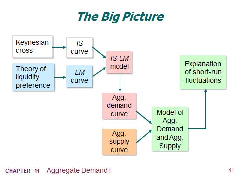
2 Plan (1) the IS curve and its relation to: the Keynesian cross the loanable funds model (2) the LM curve and its relation to: the theory of liquidity preference (3) how the IS-LM model determines income and the interest rate in the short run when P is fixed

3 Recall (1) Long run: prices flexible output determined by factors of production and technology unemployment equals its natural rate (2) Short run: prices fixed output determined by aggregate demand unemployment negatively related to output

4 Context (a) This chapter develops the IS-LM model, the basis of the aggregate demand curve (b) We focus on the short run and assume the price level is fixed (so the SRAS curve is horizontal) (c) We focus on the closed-economy case

5 The Model of Goods (Keynesian Cross) We stat from the simplest model and then making more complicated by relaxing assumptions. Easy Model: The Goods market 1 market: the market for goods and services 1 variable to determine: the level of production, or output (Y = GDP) 1 equilibrium condition to determine it: Supply of Y = Demand for Y

6 Supply of Y The economy is closed: no goods are exported or imported The price of Y is fixed P(Y ) = P = 1 Therefore $Y = Y What does this assumption mean: Output is determined by demand: at the fix price P = 1 firms produce any amount of Y needed to satisfy demand

7 Demand for Y Z Consumption(C) + Investment(I ) + GovernmentSpending(G) The 3 components of demand: Consumption is a function of disposable income (income net of taxes) C = c(y Disposable ) = c 0 + c 1 (Y T ) c 1 is the marginal propensity to consume Taxes, Government Spending and Investment are assumed to be exogenous T = T, I = I, G = G

8 Consumption Function Consumption is a function of disposable income (income net of taxes) We assume a linear relationship C = c(y Disposable ) = c 0 + c 1 (Y T ) where c 0, c 1 (c 0 > 0, 0 < c 1 < 1) are positive parameters

9 Solving the Model Variables 3 exogenous variables: T, I, G 1 endogenous variable: Y once you know Y, C = c 0 + c 1(Y T ) determines C Equations 1 equation: the market clearing condition, Y = Z With 1 equation and 1 endogenous variable the model can be solved What can move this economy away from an equilibrium? policy, shifts in T or in G shocks, shifts in firms or consumers confidence, i.e. shifts in I or c 0

10 Equilibrium in the Goods Market The equilibrium level of Y is the level that clears the market, i.e. makes supply equal to demand Y = Z = C + I + G = c 0 + c 1 (Y T ) + I + G Thus the level of Y that clears the market is Y = c 0 + c 1 (Y T ) + I + G

11 Solving for the market equilibrium C = c 0 + c 1 (Y T ) = c 0 + c 1 Y c 1 T with c 1 < 1 Solving for Y Y = 1 1 c 1 (c 0 + I + G c 1 T ) (c 0 + I + G c 1 T ) is Autonomous spending that does not depend on Y 1 1 c 1 is the Keynesian multiplier

12 The government purchases multiplier Definition: the increase in income resulting from a $1 increase in G. In this model, the govt purchases multiplier equals Y G = 1 1 MPC Example: If MPC = 0.8, then In this model, the govt purchases multiplier equals Y G = = 5 An increase in G causes income to increase 5 times as much!

13 Why the multiplier is greater than 1 Initially, the increase in G causes an equal increase in Y : Y = G But Y Y further increase in Y further increase in C further increase in Y So the final impact on income is much bigger than the initial G.

14 An increase in taxes - Solving for Y equilibrium condition: Y = C + I + G in changes: Y = C + I + G = C because I and G are exogenous = MPC ( Y T ) Collect terms with Y on the left side of the equals sign: (1 MPC) Y = MPC T Solve for Y : Y = MPC 1 MPC T [INSERT GRAPH]

15 The tax multiplier Definition: the change in income resulting from a $1 increase in T : In this model, the govt purchases multiplier equals Y T = MPC 1 MPC Example: If MPC = 0.8, then In this model, the govt purchases multiplier equals Y G = = = 4 An increase in T causes income to decrease 4 times as much!

16 The tax multiplier...is negative: A tax increase reduces C, which reduces income....is smaller than the govt spending multiplier: A change in taxes has a multiplier effect on income....is greater than one (in absolute value): Consumers save the fraction (1 MPC) of a tax cut, so the initial boost in spending from a tax cut is smaller than from an equal increase in G.

17 An exercise: the Balanced-Budget Multiplier What is the effect on Y of an increase in G fully financed by a corresponding increase in T dg = dt Y = c 0 + c 1 (Y T ) + I + G dy = c 1 (dy dt ) + dg dt = dg dy (1 c 1 ) = dt (1 c 1 ) dy = dt = dg the multiplier is 1. You still get a positive effect, but not bigger than 1: the private sector (Consumption) does not move, thus there is no multiplier effect.

18 Investment equals Saving: An Alternative Way of Thinking About Goods Market Equilibrium Start from Private Saving S Pr Y D C Y T C Now add the Saving by the Government (T G) Total Saving in the economy is S Pr + S Pu = (Y T C) + (T G) = Y C G But from Goods Market Equilibrium we know that (Y T C) = I. Thus S = S Pr + S Pu = I

19 The IS-LM Model So far the only variable in the private sector that could respond to shifts in policy (dt or dg) or in confidence (di or dc 0 ) is consumption What else could respond? prices? NOT in the Short Run. Prices are slow to respond. financial markets? YES: the price of financial assets responds instantaneously to news. We thus extend the model adding a financial sector

20 Introducing Financial Markets Financial markets include many assets with decreasing degrees of liquidity. From the most liquid (money) to the less liquid (equity) cash, demand deposits, saving deposits, money market mutual funds, government bonds, corporate bonds, equity Start from essentials. Assume there are only two financial assets money (cash, demand deposits) that pays no interest bonds that pay an interest rate i per period Think of the problem of how to allocate a given amount W between bonds and cash: the higher the interest the larger the fraction of W you will want to keep in bonds, and thus the more often you will go to the bank to sell bonds and get cash.

21 The demand for financial assets (Real) Demand for money (M d ), the most liquid asset M d P = L(Y, i) we shall assume L(Y, i) = f 1 Y f 2 i with f 1, f 2 > 0, so that M d P = f 1Y f 2 i Demand for Bonds (B d ) B d P = W Md P where W is your wealth, which is divided between money and bonds. Note: given W, if you know M d you do not need a second equation to compute B

22 "Stock" and "Flow" variables So far we have introduced two types of variables in our model Stock variables. B, W, M: these are stocks at any moment in time Flow variables. Y, C: these are measured as flows per unit time. For instance C is consumption per period, e.g. per year

23 Equilibrium in the financial market Equilibrium requires that the demand for money M d /P equals the quantity of money that the central bank has put in the economy, which we assume to be a fixed quantity M/P M d P = M P M d P = L(Y, i) = M P this equation determines the interest rate i for any given level of Y and M

24 Closing the model How does i affect the economy? We focus on one channel only: Investment Assumption: Investment depends on i, the cost firms face to borrow the funds needed to acquire new machines, build a new plant, etc. Y, the level of demand with d 1, d 2 > 0 I = I (i, Y ) = d 1 Y d 2 i

25 The IS-LM Model 4 exogenous variables: T, I, G, M 2 endogenous variables: Y, i Equations 2 equilibrium conditions equilibrium in the goods market Y = Z equilibrium in the financial market M d /P = M/P With 2 equations and 2 endogenous variables, the model can be solved What can move this economy away from an equilibrium? policy, shifts in T, G, M shocks, shifts in firms or consumers confidence, i.e. shifts in I or c 0

26 Solving the IS-LM Model Two equations equilibrium in the goods market gives you the IS Curve Y = Z Y = Y (i) equilibrium in the financial market gives you the LM Curve M P = M P i = i(y ) two equations and two unknowns: the model is solved

27 Solution of the Model IS-LM 2 equations: (1) the equilibrium in the market of goods results in the IS equation Y = Z Y = Y (i) (2) the equilibrium in the financial market M d P results in the LM equation = Ms P i = i(y ) 2 equations and 2 unknowns: the model has a solution! [GRAPH]

28 The Short-Run Equilibrium LM equation: IS equation: M s P = f 1Y f 2 i i = f 1 Y Ms f 2 P Y = c 1 (Y T )+c 0 +d 1 Y d 2 i +G Y = c 1T + c 0 d 2 i + G 1 c 1 d 1 Replace i from the LM equation into the IS equation, to obtain: 1 f 2 [GRAPH] Y E = c 1T + c 0 d 2 M s f 2 P + G f 1 c 1 d 1 + d 1 2 f2 i E = f 1 Y E Ms f 2 P 1 f 2

29 Multipliers the IS-LM Model dy dt = c 1 (1 c 1 d 1 ) + d 2 f 1 f2 < 0 dy dg = 1 > 0 f (1 c 1 d 1 ) + d 1 2 f2 dy dm = 1 (1 c 1 d 1 ) f 2 d 2 + f 1 > 0

30 Summary (1) Keynesian cross basic model of income determination takes fiscal policy and investment as exogenous fiscal policy has a multiplier effect on income (2) IS curve comes from Keynesian cross when planned investment depends negatively on interest rate shows all combinations of i and Y that equate planned expenditure with actual expenditure on goods and services

31 Summary (3) Theory of liquidity preference basic model of interest rate determination takes money supply and price level as exogenous an increase in the money supply lowers the interest rate (4) LM curve comes from liquidity preference theory when money demand depends positively on income shows all combinations of i and Y that equate demand for real money balances with supply

32 Summary (5) IS-LM model Intersection of IS and LM curves shows the unique point (Y, i) that satisfies equilibrium in both the goods and money markets

33

34 Part of the slides are taken from MIT OpenCourseWare Course: Francesco Giavazzi Principles of Macroeconomics, Spring (Massachusetts Institute of Technology: MIT OpenCourseWare), (Accessed 22 Aug, 2015). License: Creative Commons BY-NC-SA