Theory of Consumer Behavior First, we need to define the agents' goals and limitations (if any) in their ability to achieve those goals.

Transcription

1 Theory of Consumer Behavior First, we need to define the agents' goals and limitations (if any) in their ability to achieve those goals. We will deal with a particular set of assumptions, but we can modify them in a number of different ways. We will then try to infer something about the agent's behavior. The behavior is going to be a description of choices that people make as a function of the constraints they face.

2 Goals There are three different ways of approaching the problem of consumer choice. The most traditional way is to suppose that there is something called utility or satisfaction. Consumers get satisfaction from engaging in certain economic activities. The utility function measures the amount of satisfaction that the individual gets from a market basket with n different commodities indexed by 1, 2,...,n The amount of each of these commodities in the basket or bundle is be represented by the number x i where i = 1,...,n. So, a basket of goods would be an n dimensional vector x = (x 1,...,x n )

3 We can think about the utility function as a function that assigns to each bundle of goods some real number denoting the amount of utility obtained from a bundle: U: x R For example, if n=2, then a bundle (x 1, x 2 ) is a point in a two dimensional Euclidean space that denotes a certain amount of good 1 and a certain amount of good 2 (say ham and eggs).

4 The goal of the agent would then be to choose that bundle giving the greatest level of satisfaction or utility. We can make further assumptions regarding utility. I may assume that it is monotone, i.e. at any point in the space if I move northeast, I am better off (more is better). Under certain circumstances we may wish to relax this assumption - there is a limit to how much cherry vanilla ice cream I can enjoy at a single sitting! With two different commodities, if we draw a utility function as a height in a three dimensional space, we get a "mountain" over the plane containing the different bundles.

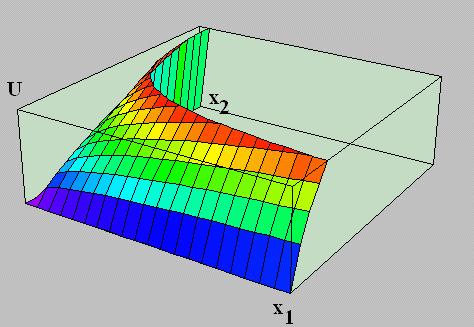
5

6 To be able to see this in a two-dimensional drawing, we can "slice" the mountain at a certain height and obtain a line connecting all points that give you the same level of utility. That line would be called an indifference curve. There are an infinite number of indifference curves.

7 Any two bundles (say x 1 and x 2 ) on the same indifference curve, give me the same level of utility. In this case we can write that U(x 1 )=U(x 2 ). An indifference curve consists of the set: {x U(x)=U o } where U o is a constant. Say I am at a particular point and I want to find the slope of the indifference curve. Implicitly, in this function I have U(x 1, x 2 (x 1, U o )) U o Given x 1, the indifference curve associated with U o are those values of x 2 which produce U o Since this is an identity, I can differentiate with respect to x 1 and both sides will remain equal.

8 If we change x 1, utility changes because x 1 is the first argument of the utility function and utility depends directly upon it. But if I change the first argument and stay in the same indifference curve, x 2 has to change. So, the change in x 1 is going to induce an indirect change in utility through the change in x 2 that keeps me on the same indifference curve. I can solve this expression for x 2 / x 1 (which is the slope) and I find that : where U 1 = U / x 1 (the additional utility from of another unit of good 1, or the marginal utility of good 1); and U 2 = U / x 2.

9 This tells me that the slope of this indifference curve is equal to the ratio of the additional utility you get from one good relative to the other. What it tells us is how much of good 2 I need in order to replace a unit of good 1. (If I have one less unit of good 1, how much more of good 2 would I need to leave me just as well off as I was with the original bundle). It tells me the rate at which I am willing to trade one good for the other. If the slope is very flat, it tells me that in order to give up one unit of the vertical good I need to give up a lot of the horizontal good. The opposite is true if the slope is very steep. So how I value one good relative to another depends on where I am in the space and in particular on the proportions of the goods in the bundle.

10 The ratio at which I am willing to trade one good for another is the marginal rate of substitution (MRS). If I give up one unit of good 1, how much utility do I lose? I lose a level of utility equal to U 1. How many units of good 2 do I need to make up for that loss of utility? I need U 1 /U 2. The MRS is the slope of the indifference curve at a certain point. It says how much of good 2 I can give up if I get one more unit of good 1 and I want to stay on the same indifference curve. For example, if U 1 =10 and U 2 =5 and I give up a unit of good 1, I loose 10 units of utility and I need 2 units of good 2 to make up for the 10 units of lost utility.

11 Examples of Indifference Curves. If my MRS does not depend on how much of the goods I am consuming, then the goods are perfect substitutes. For example, a unit of good 1 always changes for two units of good 2 along an indifference curve. (In most dishes, for example, it doesn t matter if you cook with corn oil or sunflower oil, so these goods are substitutes.) If the goods are perfect complements, then one good is only useful with the other one (left and right shoes). Usually when we draw an indifference curve, we make an assumption that the goods have a diminishing MRS. As I move along the indifference curve and I get more of good 1 and less of good 2, the relative value of good 1 declines.

12 Substitutes Complements Diminshing MRS

13 Constraints - The Budget Set. Assuming that more is better, I want unlimited amounts. But there are limitations: I can buy as many eggs as I want and as much ham as I want as long as I can afford them. Say I = income level p 1 = price per unit of good 1 p 2 = price per unit of good 2 The bundle of goods that I can afford is: x=(x 1, x 2 ) where I p 1 x 1 + p 2 x 2

14 If I have more than two commodities, I can afford a bundle x if p x I. Remember that the dot product p x is equal to:. Another way of writing the same thing is: B(p, I) = {x p x I} Graphically, we have I/P 2 I/ P 1

15 If I spend all my income, then where I = p 1 x 1 + p 2 x 2. I can afford anything on that budget line or below. The slope of this budget line tells me how many more units of good 2 can I buy if I buy 1 unit less of good 1. Another way of saying this is that this is the opportunity cost in terms of good 2 of consuming a unit of good 1. At the corners (I/p 2 and I/p 1 ) I spend all my income on only one good.

16 The Individual's Decision Problem. Given preferences and given the constraints, the individual wants to get to the highest level of satisfaction or highest indifference curve possible (by assumption).

17 At point A, I know that U 1 / U 2 < p 1 /p 2 (since the indifference curve U 1 /U 2 is flatter and the budget line p 1 /p 2 is steeper). In other words, the MRS is less than the opportunity cost. U 1 / U 2 is the amount of good 2 that I need in order to replace a unit of good 1, and p 1 /p 2 is how much of good 2 I can buy if I give up a unit of good 1. This tells me that if I give up a unit of good 1, I can get more of good 2; this will provide more utility than the utility lost from consuming one fewer unit of good 1. This means that I could do better by consuming less of good 1 and more of good 2. I can increase my utility by giving up some of good 1, moving in the direction of the arrow until I reach point B. At point B, we have U 1 / U 2 = p 1 /p 2, and the budget line and indifference curve are tangent. In that case I could not do better by moving in any direction.

18 In other words, if I face fixed prices, I am going to adjust the amounts of the goods I consume until at the margin, I value the goods myself in the same way as their opportunity cost. I am going to adjust my consumption of ham and eggs until I value ham and eggs in the same way the market does. After everybody adjusts their consumption to spend their money on ham and eggs optimally, everybody will end up valuing ham and eggs the same way at the margin. (Remember that we are dealing only with two goods). People will achieve this in different ways. Some people will achieve this by consuming a lot of ham and very little eggs, and some will need to spend equal amounts of each; however, at the margin everybody will value ham and egg in the same way. My MRS between ham and eggs is the same as yours since we face the same prices.

19 Corner solution. An exception to the above is when we do not have an interior internal solution. For example, say there is someone who does not like the horizontal good ve ry much.

20 The best this person can do is to consume at point A. However, at that point the slopes are not equal (U 1 / U 2 < p 1 /p 2 ). The market would give me more of good 2 for a unit of good 1 than I need to be just as well off. So I should give some of good 1 and get more of good 2, but I have no good 1 to offer. So for all goods that the individual consumes in positive amounts, the individual values them at the same rate ratio as the market prices.

21 Preferences and the Utility Function. So far we have only used the ratio of the marginal utilities of good 1 and to good 2 (the slope of the indifference curves). We have not used the magnitude of the amount of satisfaction. Remember that measures of utility are not important. Rather, the ranking of the bundles is what matters. Let s assume I change the utility function in such a way that I keep the same indifference curves. I can do that by taking any positive monotone transformation f of U (defined as a function such that df/du > 0) to transform the old utility measure U(x) into a new one V(x). f(u(x)) = V(x)

22 Bundles with Whatever got higher levels of utility using U(x) will also get higher levels of utility under V(x), and any two bundles a and b s.t. U(a)=U(b) will also satisfy V(a)=V(b). Therefore, the indifference curves will not change. To be sure, the measure of utility or their height will change, but bundles on whatever was the same indifference curve height before, will continue to be at the same one now. The slope of an indifference curve does not depend on how we measure utility (with a monotone transformation). Let's look at it in a different way. The MRS using utility U(x) is - U 1 / U 2, and the MRS using V(x) is - V 1 /V 2. But we know that: since f'>0.

23 So instead of thinking about individuals having utility functions, we may think of individuals as having preference orderings. We can talk about x 1 x 2 where " " reads "at least as good as". Under certain conditions, we could find an ordinal utility function that gives the same information as these preference orderings. If I can get the same information with either technique, I do not lose anything by describing preferences by a utility function. The three conditions that these preferences have to meet for the existence of such a utility function are: such equivalence are:

24 (1) The ordering of the preferences are complete. This means that you can compare any two bundles. You can say either x 1 x 2 or that x 2 x 1 (2) Transitivity. If x 1 x 2 and x 2 x 3, then x 1 x 3 There are no loops. An example of a decision process that gets you in loops is the following: Suppose that I have criteria for judging goods. In order to make a decision I "take vote within myself" (that is, if one bundle is better than the other two in two out of the three criteria, then I like that one better). Let's say the order of my preferences under each criteria is: Criteria 1 Criteria 2 Criteria 3 A B C B C A C A B

25 This means that if: and transitivity fails. A B; B C; C A If I vote one good against another and the winner against the third one, I get 3 different results depending on the order in which I vote on them. In this case, my goals are not well defined and I cannot apply this methodology. (3) Continuity. This is a mathematical condition but, for Euclidean consumption spaces, it states that given three bundles A, B and C where A B C then there is a convex combination of A and C which is judged to be indifferent to B, i.e. s.t. 1 and A+(1- )C is indifferent to B. If my preferences are complete, transitive, and continuous, then I can find an equivalent ordinal utility function that will order bundles in the same way. So I can talk interchangeably say that A is at least as good as B or U(A)>= U(B).about preferences being "as good as" or I can talk about an ordinal utility function.

26 Our Problem Now we will look at the constrained maximization problem but we will look at it algebraically and using the techniques of Lagrangian multipliers. I have a utility function U(x 1, x 2 ) which depends on the amount of x1 and x2 that I buy. The problem we want to solve is: Max U x, x s.t. p x p x I s.t. s.t. x x

27 Suppose I want to solve a problem where I want to maximize U(x 1,x 2 ) and spend all my income so p 1 x 1 +p 2 x 2 = I (I want to be on the thick line in figure 2). x 2 I = p 1 x 1 + p 2 x 2 x 1 To solve this problem, we form a Lagrangian expression: To do this we must first re-write the constraint as I p 1 x 1 p 2 x 2. We can then write the Lagrangian Expression as follows. U(x 1, x 2 ) + (I p 1 x 1 p 2 x 2 ) and find the unconstrained saddle point to this expression.

28 The FOC are: U 1 p 1 = 0 U 2 p 2 = 0 I p 1 x 1 p 2 x 2 = 0 (Remember that in a maximization or minimization problem the FOC say that the first derivatives are equal to zero and the second order conditions talk about the function being concave or convex). To solve these three equations I can set the first two equations equal to and I get: = U 1 / p 1 = U 2 / p 2. Which can be rewritten as: U 1 / U 2 = p 1 / p 2 (We saw earlier that this expression means that the MRS was equal to the opportunity cost). So, we now have two equations and two unknowns: U 1 / U 2 = p 1 / p 2 p 1 x 1 + p 2 x 2 = I

29 The interpretation of. If I have a dollar, I can buy 1/p 1 units of good 1. Since U 1 is the utility I get for spending a dollar on good 1, U 1 / p 1 is the amount of utility that I can get by spending the marginal dollar on good 1. Similarly, U 2 / p 2 is the amount of utility that I can get by spending the marginal dollar on good 2. We just saw that in order to really maximize my utility, these two expressions have to be equal. This means that I have to be getting as much satisfaction spending a dollar on good 1 as I get spending it on good 2, or in other words, if I have a dollar, I get the same level of satisfaction by spending it on any of the goods. So, can be interpreted as the additional satisfaction that I would get from an additional unit of income.

30 In general, the Lagrangian multiplier associated with a specific constraint tells us how much more we can achieve in the criteria function if the constraint is weakened by one unit. It tells us how much the thing that is scarce is worth in terms of what we are trying to achieve. The process we just described will be the standard way of attacking most of the problems we will encounter. Because most of these problems will have a goal that can be described as some real valued function f(x) and one or several constraints that can be described as inequalities.

31 Another Example (Shadow Price) Suppose I own a business and I use only one input. I want to maximize my profit subject to the constraint that I cannot use more than a certain amount of the input. That is: Max pf(x) s.t. x x. Where f(x) is the production function, p is the price of the good and x is the input. To solve this problem we set the Lagrangian: L pf(x) (x x). Then we differentiate with respect to x and set it equal to zero. So our FOC are: pf '(x) ~ ~ and ~ x x. The meaning of ~ in this case is the additional profit that I could get if I had one more unit of x. It is the shadow price of another unit of x. It is not a price in the usual sense, but rather the extra revenue (profit) from relaxing the constraint of how much of the input I can use.

32 A numerical example Maximize the utility function subject to the given budget 1 4 U(x,x ) x x constraint. The utility function is: And let's say that: p 1 = 2, p 2 = 4, and I = 12. Then the Lagrangian can be written as: L=U(x 1, x 2 )+ (I-p 1 x 1 -p 2 x 2 ) or L=x.25 1 x (12-2x 1-4x 2 ) 1 2 FOC U 1 p x x U 2 p x x x 1 4x 2 12

33 If we eliminate we get: 1 2 x 1 4 x x x 2 Which means that x x Replacing this result in the third equation we get ~ x ~ x 2 1 2

34 The marginal utility of income is: x x ~ 1 2 2, 4 where we substitute x 1 and x 2 with 2. Note that cannot be negative. If it did, it would mean that using up my constraint was costing me utility (I could do better if I do not use up all the constraint).

35 Quick review of what we have done. The general Lagrangian multiplier technique was as follows. If we want to maximize a utility function U(x) subject to p i x i I, we set up a Lagrangian expression: U( x) ( I px) and then take the first order conditions: U (x) ~ ~ p 0 i i If any of these equations is less than zero, then ~ x i 0. i

36 The first order conditions can also be written as: U i / p i i. In this case, if U i / p i is less than then ~ x i 0. For any good we were consuming in positive quantities, could be interpreted as the additional utility that we could get by spending a dollar on that good. Note that in this story there is only one period, so saving money does not give us utility, and we cannot borrow. The results we got were the same than the ones we had seen graphically, when we said that if we wanted to maximize utility subject to a budget constraint we would end up at a point where the indifference curve was just tangent to the budget constraint: U 1 U 2 p 1 p 2

37 Several constraints If we have more constraints, we just add another Lagrangian multiplier. In this case we need to be at a minimum with respect to each Lagrangian multiplier and at a maximum with respect to x. For example, suppose things were rationed and we needed not only money to buy things but also coupons. Our Lagrangian would look like: U(x) (I px) ( C qx) In this case is the additional utility that I would get for an additional unit of income and is the additional utility that I would get for an additional coupon. I can only buy something if I have the money and the coupon. I am restricted to the shaded area in figure 1.

38 If my maxima is at point A, the shadow price of coupons is zero. Similarly if my maxima is at point B, I did not use all my money but I ran out of coupons. The shadow price of money is zero. At point C we run out of both money and coupons. x p x = I B C q x = C A x 1

39 First and second order conditions Diminishing marginal utility means that the indifference curves bow inwards like in the figure on the left. However, I can have an indifference curve that bows inward and still have a maxima (given my budget constraint). But if I do not have diminishing marginal rate of substitution, I might not have a unique maxima (see figure above on right)

40 If the indifference curve looks like those below, then there are two points on the budget line where the MRS equals the ratio of prices. However, both are not maxima. One is clearly on a higher indifference curve than the other. The FOC, namely that the MRS equals the ratio of prices, is a necessary but not sufficient condition for utility maximization.

41 Different shapes of budget constraints If my budget constraint looks like the one below, I still will have the same FOC: the slope of the indifference curve must equal the slope of the budget line. The slope of the budget line is still going to give me opportunity cost of one good in terms of another. Constraint

42 Effects of changes in income After we maximize an individual s utility subject to a constraint, we end up with a choice that the individual makes. Below the choices under the lower-income and higher-income budget sets are x and x, respectively. x 2 X (p, I) x' x 1

43 If we change prices or income, we change the highest point that the individual can reach. For example if we have less income, the new budget line would be parallel but lower, and the new choice would be x If we want to infer something about how demand behavior changes when we alter the income constraint (and keeping prices constant) we get a graph like this:

44 In this figure x 1 is measured on the horizontal axis, and x 2 is measured on the vertical axis. Therefore we can see the demand for a good at each level of income. If we connect all such points, we get an income consumption (or expansion) path.

45 Associated with this, I can draw the Engel curve where I have income on the horizontal axis and the demand for, say the first good, on the vertical axis. The Engel curve is basically the demand for a good as a function of income, holding all else constant. x 1 I

46 Holding prices constant, if we increase the level of income and the consumption of the good increases, we call it a normal good (for example, good 1 in in the graph on the last slide). However, if when income increases the consumption of the good decreases, we call it an inferior good. (For example, good 1 in the figure below). Good 2 Good 1

47 Some examples of inferior goods, are things that allow us to stay alive without spending much money (such as Spam). If our income increases we switch to a good that we like better but that we could not afford before. A note on assumptions. Two people, with different assumptions about the way the world is set up, can look at the same data and come up with widely different conclusions. We need to remember that the assumptions that we make affect the conclusions we reach even if the data we work with does not change. The assumptions we make as well as the models we work with will affect the conclusions we reach. On the other hand, there is no way of looking at data or facts about the world without having some theoretical model --some way of organizing that data-- in your thoughts. You have to have some idea of the way things go together in order to be able to make sense of the data that you look at.

48 Effects of changes in prices Now we want to see how demand changes when we change prices. Let s say the prices of good 1 varies (see figure 10). If we connect again all tangency points, we obtain a price consumption curve. X 2 X 1 p 1 x 1 (p 1, p 2, I ) x 1

49 I can also ask what happens to the demand of good 1 as I vary the price of good 1 (holding income and the price of good 2 constant as we did on the last slide). We obtain a Marshallian demand curve. Note that this time we have quantity on the horizontal axis and prices on the vertical axis p 1 x 1 (p 1, p 2, I ) x 1

50 Could demand curves slope upwards? Keep in mind that we have to play with the rules of the game. The rules say that utility just depends on the physical amount of the goods consumed and that price does not enter the utility function. Therefore, an example in which I get utility from a good just because it is more expensive violates the assumptions of the model we are working with. This is an important question because one thing that economist like to do is comparative statics. P S P* D Q

51 We want to focus on P* as the outcome from this market. We justify it with the following story: if price is greater than P*, there would be an over supply of the good and that would push the price down. If we are below that price, there would be an excess demand and that would push the price up. However, if the demand curve looked differently, an over supply could push prices down and an over demand could push prices up (see figure below). P S D P* Q

52 In this case, P* is still the price in equilibrium, but it is not the price that other prices converge to. Downward sloping demand curves and upward sloping supply curves give us a sufficient condition for this type of stability property. Have we made any assumptions that allow us to conclude that individual demand curves could slope upwards? Suppose we have the following case: Good 2 Good 1

53 When the price of good 1 goes down, I am relatively richer so I buy more of good 2. And since good 1 is an inferior good, as the price of good 1 goes down, we become relatively richer so we buy less of it. Imagine that there are two goods: rice and meat. I would like to be getting all of my food from meat. However, meat is very expensive and rice is very cheap. I am so poor that if I tried to buy only meat I could not keep myself alive. So I buy mostly rice. If the price of rice falls, I could buy as much rice as I did before and have a little left for additional meat. I could even buy less rice that I did before and spend all of the difference on meat and be better off than I was before.

54 In conclusion, we can see this behavior if: (1) we are dealing with an inferior good; (2) we spend most of our income on it; and (3) there is no close substitute. A good whose quantity demanded increases as its price increases is called a Giffen good (sometimes this is referred to as the Giffen s paradox). A Giffen good must be an inferior good, but an inferior good is not necessarily a Giffen good.. The things we have talked about so far are local properties of the demand function. They are descriptions about what is happening to this function at a particular point. For example, a good could be a Giffen good for some prices and a normal good for others.