Risky Human Capital and Alternative Bankruptcy Regimes for Student Loans

Transcription

1 Risky Human Capital and Alternative Bankruptcy Regimes for Student Loans Felicia Ionescu November 2009 Department of Economics, Colgate University, 13 Oak Dr, Hamilton, NY, 13346, USA. Abstract I study the effects of uncertain human capital investment and alternative bankruptcy regimes on college enrollment, completion and life-cycle human capital accumulation. Findings suggest that risky college education results in less human capital investment. Individuals with relatively low ability and low initial human capital levels are affected to a greater degree by this risk. A correlation between ability, initial human capital and financial assets is important in delivering enrollment and completion rates across initial assets groups consistent with empirical findings. The option to discharge one s debt under a liquidation regime helps alleviate some of the risk of investing in human capital, in particular for students with low initial assets, for whom the risk of investment is highest. Thus dischargeability induces more human capital accumulation over the life-cycle relative to a reorganization regime, where dischargeability is not allowed. JEL classification: D91; G33; I22 Keywords: Bankruptcy; Student loans; College Risk Thanks to participants at Macro Midwest Meetings, Midwest Economics Meetings, seminar series at Colgate University, Fordham University, University of Connecticut, University of Delaware, University of Western Ontario, and Macro Workshop of Liberal Arts Colleges, especially to Kartik Athreya, S. Chattarjee, Dean Corbae, Dirk Krueger, Lance Lochner, Igor Livshits, B. Ravikumar, Nicole Simpson, Chris Sleet, Jorge Soares, Gustavo Ventura, Galina Vereschgagina, Steve Williamson, Eric Young, and Christian Zimmermann. Tel.: (315) ; fax: (315) ; address: fionescu@mail.colgate.edu 1

2 1 Introduction More than 10 million people borrowed $66 billion under the Federal Student Loan Program (FSLP) in fiscal year The risk associated with taking out a student loan and investing in college is far from being negligible. 2 Moreover, default rates for student loans averaged 12% in the last two decades with the highest rate of 22.4% in 1990 (a 2-year basis cohort default rate). A rapid increase in personal bankruptcy filing rates with a historic high of 9.15% in 2005 turned researchers focus, however, on the nation s bankruptcy laws and risky behavior in the unsecured credit market. Little attention has been given to analyzing risky human capital investment in conjunction with bankruptcy rules in the student loan market. Yet, an understanding of the mechanism behind the risk associated with investment in human capital and evidence about students responses to the incentives created by bankruptcy laws would help policy makers as they work to redesign the student loan program. 3 This paper studies the effects of risky human capital investment under alternative bankruptcy regimes for student loans on college enrollment, completion and life-cycle human capital accumulation across different groups of high-school graduates. I develop a heterogeneous life-cycle economy where agents differ in initial ability, human capital stock and financial assets. Agents decide to invest in their human capital during college as well as after college, as on-the-job training. They may need to borrow under the FSLP to invest in college and consequently they need to repay on their college loans after college. This model builds up on Ionescu (2009), who, in turn generalizes the Ben-Porath (1967) human capital model and studies college enrollment, borrowing and repayment behavior under the FSLP. The paper abstracts, however, from accounting for the risk of human capital investment and alternative bankruptcy arrangements (liquidation versus reorganization), the focus of the current study. The current paper takes a further step in the analysis of college investment and default incentives by incorporating the risk of dropping out from college along with the option to discharge student loans. Uncertainty in employment prospects after college may deter some students from investing in human capital. In addition, the option to discharge one s debt may provide partial insurance against employment risk after college. My results shed light on these issues and to my knowledge, they represent a first effort in the literature to provide insights regarding risky human capital accumulation and the role of dischargeability 1 In the same year total unsecured debt amounted to $939 billion. 2 Using the PSID 1990, Restuccia and Urrutia (2004) find that 50% of people who enroll in college drop out. According to the NCES data, 36.8% and 35.2% of people enrolled in college in 89/90 and 95/96, respectively do not have a degree and are not enrolled 6 years after enrollment. 3 High default rates in the late 1980s have led legislators to introduce a series of policy reforms that gradually made student loans nondischargeable, in switching from Chapter 7, a liquidation chapter in the Bankruptcy Code to Chapter 13, a reorganization chapter. 2

3 to alleviate this risk. More specifically, in this environment risky college education results in less college enrollment and less human capital investment in general relative to an economy where college investment is not risky. People with relatively low initial ability and human capital levels are affected to a greater degree by the risk of dropping out from college. The ability level drives the decision to enroll in college, while the initial human capital level is crucial for completing college. A positive correlation between ability and initial financial assets is important in delivering enrollment rates consistent with empirical findings, whereas a positive correlation between initial human capital and initial financial assets is key in delivering accurate completion rates. Results also suggest that the option to discharge one s debt helps reduce the risk of investing in college. In particular, dischargeability benefits students with low initial financial assets and human capital levels; these are precisely the students for whom the risk of college investment is highest. Thus, a liquidation bankruptcy regime that allows for dischargeability induces more college enrollment, although it raises default rates. Given the uncertainty in post-college earnings in the U.S., the model suggests that a liquidation regime induces higher levels of human capital over the life-cycle, and thus, higher earnings profiles relative to a reorganization regime, where dischargeability is not allowed. 1.1 Literature This paper ties two directions of study in the literature: human capital; and bankruptcy. The first line of research has been extensively explored with most of the interest directed toward the relevance of students initial characteristics for human capital investment and optimal policies for financially-constrained students. Ben-Porath (1967) and Becker (1964, 1993) are among the first studies to recognize the importance of the complementarity between ability and human capital stock in explaining life-cycle human capital accumulation and earnings dynamics. The Ben-Porath framework has been further exploited in this direction by Huggett, Ventura, and A.Yaron (2006) who show that the model can replicate the U.S. earnings distribution dynamics using the right initial distribution of characteristics. Their model does not incorporate schooling decisions and does not distinguish between investment across different education groups. Recent studies summarized in Heckman and Carneiro (2003) document, however, that most of the human capital investment takes place at the beginning of the life-cycle during the schooling period and it is followed by subsequent learning during the life-cycle as on the job training. Heckman, Lochner, and Taber (1998) also extend the Ben-Porath framework and model schooling decisions to study the rising in 3

4 wage inequality by education groups. Their approach, however, assumes that the earnings of agents in the model match earnings in the data for individuals sorted by a measure of ability such as AFQT scores and whether they attended college. Consequently, the contribution of schooling to subsequent investment in human capital is embodied in schooling specific skills and endowments. These studies do not incorporate the risk in human capital investment. Yet, research demonstrates that a substantial fraction of the variability in the returns to schooling is unpredictable at the time when schooling decisions are made, implying that this uncertainty is not due to differences in initial characteristics by the time students decide to go to school (see Cunha, Heckman, and Navarro (2005) and Palacios-Huerta (2003)). More recent papers incorporate the risk of human capital investment to focus on optimal policy, but most of the attention is directed on optimal taxation policy (see Grochulski and Piskorski (2009) and Krebs (2003)). Finally, there is large body of this literature that emphasizes the relevance of credit constraints for schooling decisions (see Carneiro and Heckman (2002) and Keane and Wolpin (2001)). The current paper is in line with the human capital literature in the following ways: it recognizes the importance of both human capital stocks and ability for life-cycle human capital formation and earnings; it distinguishes between investment in human capital during schooling and job training periods; it allows for heterogeneity in financial assets along with individual characteristics; and most importantly, this study accounts for the risk in human capital investment and analyzes the means to mitigate this risk, such as dischargeability of student loans. To this end, the human capital literature has ignored in general the relationship between human capital investment and default incentives for student loans. Exceptions include work by Lochner and Monge (2008) and Ionescu (2009). The first paper studies the interaction between borrowing constraints, default, and investment in human capital in an environment based on the U.S. Guaranteed Student Loan Program 4 and private markets where constraints arise endogenously from limited repayment incentives. The second paper quantifies the effects of repayment flexibility (such as to lock-in interest rates or to switch repayment plans) and the relaxation of eligibility requirements for student loans on enrollment and default rates in an environment based on the FSLP. The current study differs from both of these papers in several important ways. First, I account for the risk of college education and study college enrollment and completion across groups of high-school graduates. In addition, I incorporate work during college, which proves to be one of the main factors for dropping out from college (see GAO (2003a) and Tinto (1993)). Furthermore, I analyze the incentives created by alternative bankruptcy regimes, which is key for the analysis of risky human 4 GSL is the former FSLP with a different set of rules upon default 4

5 capital investment. Finally, I allow for heterogeneity in financial assets, ability and human capital and calibrate the life-cycle model to capture the correlation between financial assets and unobserved characteristics to deliver college enrollment and completion behavior by groups of financial assets consistent with the empirical evidence. Research on bankruptcy has focused on personal bankruptcy laws and their implications for filing rates with significant contributions by Athreya (2002) and Chatterjee et.al.(2007). These studies explicitly model a menu of credit levels and interest rates offered by credit suppliers with the focus on default under Chapter 7 within the unsecured credit market. The literature has abstracted in general from studying bankruptcy under both regimes in the U.S. An important contribution by Livshits, MacGee, and Tertilt (2007) incorporate both bankruptcy regimes, contrasting liquidation within the U.S. to reorganization in Europe in a life-cycle model with incomplete markets with earnings and expense uncertainty. The current paper simulates bankruptcy characteristics of the student loan market, which are very different than those of the unsecured credit markets. Student loans are not secured by any tangible asset, so there might be some similarities with the unsecured credit market, but unlike those types of loans (credit cards), guaranteed student loans are uniquely risky, since the eligibility conditions are very different. Loans are based on financial need, not on credit ratings and are subsidized by the government. 5 Agents are eligible to borrow up to the full college cost minus expected family contributions. More important, unlike interest rates in other credit markets, the interest rate on student loans does not incorporate the risk that some borrowers might exercise the option to default. The feedback of any bankruptcy law into the interest rate is exactly how the default is paid for. I endogenize the bankruptcy decision and I consider the default penalties similar to those implemented in the actual program, that might bear part of the default risk. 6 To my knowledge, this is the first paper to study the effects of the risk of human capital investment and alternative bankruptcy regimes on college enrollment, completion, and default incentives for student loans along with the consequences for human capital accumulation over the life-cycle. The paper is organized as follows: Section 2 provides background on the bankruptcy rules for student loans; Section 3 describes the model and Section 4 the parametrization procedure; I present the results in Section 5 and conduct a sensitivity analysis in Section 6; I conclude in Section 7. 5 The FSLP consists in both subsidized and unsubsidized loans. Research shows, however, that all government loans are heavily subsidized (see Lucas and Moore (2009)). 6 This unique feature of the student loan market allows me to focus on default consequences under alternative bankruptcy regimes in a partial equilibrium setup where price effects are not accounted for. 5

6 2 Bankruptcy under the FSLP Bankruptcy in the model is closely related to Chapter 7, The Liquidation Chapter and Chapter 13, Adjustment of the Debts of an Individual With Regular Income, one of the Reorganization Chapters under the Bankruptcy Code. The most significant distinction between them is in regard to the administration of the estate. Rather than a disposal of the assets through liquidation sale, the purpose of the reorganization chapters is to preserve and protect the integrity of assets from the claims of creditors, so as to permit the debtor an opportunity to reorganize and restructure his assets and liabilities and to become economically viable. The main differences between the consequences to default on student loans under the two regimes are: (1) Under liquidation the loan is discharged, whereas under reorganization a repayment plan is implemented. Debt can increase by as much as 25% of the principle at the time when default occurs. The defaulter loses his right to consolidate after default, so paying under no-consolidation status is the only available option for the borrower who enters repayment in the following period after default occurs; (2) Under liquidation, defaulters are excluded from credit markets, whereas under reorganization bad credit reports are erased and credit market participation is not restricted once the borrower starts repaying; 7 (3) The wage garnishment is interrupted under reorganization once the defaulter enters repayment. The garnishment continues for several years under liquidation. These differences between the two bankruptcy regimes are summed-up in Table 1. Table 1: Bankruptcy rules under FSLP Chapter 7 - Liquidation Chapter 13 - Reorganization Purpose Disposal of the assets Protection of the assets integrity Dischargeability Allowed Not allowed Cost Wage garnishment Wage garnishment Exclusion from credit markets Debt increase Seizure of tax refunds Seizure of tax refunds Loss of consolidation rights Benefit Loans discharged Bad credit report erased Students who participated in the Federal Loan Program before 1990 could file for bankruptcy under Chapter 7 without any restrictions and could discharge on their loans. In this paper I refer to this period as liquidation. Dischargeability was initially limited in 1990 by the 7 Failure to repay a defaulted student loan can be damaging the credit record of the defaulter for 10 years (Chapter 7) or 7 years (Chapter 13). However, under reorganization, the negative credit report made by the Department is removed in the case the defaulter successfully rehabilitates his loan. Based on the discussions with financial aid agencies, most of the defaulters enter repayment and rehabilitate their defaulted loans. 6

7 Student Loan Default Prevention Initiative Act to one of the two cases: (1) if the first payment on the student loan became due more than 7 years before the filing of the bankruptcy petition or (2) if it would cause undue hardship on the debtor. The Higher Education Amendments to the Bankruptcy Code in 1998 eliminated the 7-year discharge basis, keeping undue hardship as the only basis for obtaining a discharge. After the reforms, students cannot discharge on their loans anymore. They file for bankruptcy under Chapter 13 and enter a repayment plan. The indebted defaulter is required to reduce consumption to finance at least partial repayment of his obligations. Availability of discharge is limited, so I refer to this period as reorganization. 8 Under the current program students start to repay their loans six month after graduation. The interest rate on education loans is set by the government and it is based on the 91-day Treasury-bill rate. Thus, it fluctuates with the market. Borrowers start repaying under the standard plan that assumes fluctuating payments. 9 If they do not make any payments within 270 days in the case of a loan repayable in monthly installments or 330 days in the case of a loan repayable in less frequent installments, they are considered in default, unless an agreement with the lender is reached (Section 435(i), Title IV of the Higher Education Act). Default status is reported to credit bureaus. Penalties on defaulters include: garnishment of their wage, seizure of federal tax refunds, possible hold on transcripts, ineligibility for future student loans, bad credit reports that exclude them from other credit markets. 10 The Department of Education and student loan guaranty agencies are authorized to take ( garnish ) a limited portion of the wages of a student loan debtor who is in default. Due to recent changes in the law, the Department may garnish up to 15% of the defaulter s wages (The Debt Collection Improvement Act of 1996). Wage garnishment could be avoided if it would result in an extreme financial hardship for the defaulter. I will adjust the garnishment relative to the minimum income. In addition, once the defaulter rehabilitates his loan, the wage garnishment is interrupted. The IRS can intercept any income tax refund the defaulter may be entitled to until student loans are paid in full. This is one of the most popular methods of collecting on defaulted loans, and the Department of Education annually collects hundreds of millions of dollars this way. Each tax year, the guaranty agency holding the defaulter s loans must review the account to verify that the defaulter has not made any 8 As a practical matter, it is very difficult to demonstrate undue hardship unless the defaulter is physically unable to work. The 7 year basis discharge is not relevant to the current study as filing for bankruptcy within my data and model occurs within two years after graduation. 9 Borrowers can switch to a different repayment plan. In the current study I abstract from modeling other repayment options to analyze the impact of the default option in isolation under alternative regimes. For a study on repayment options see Ionescu (2008). 10 Institutions with high default rates are also penalized, but since I focus on the individual decision, this punishment is not captured in the current study. 7

8 loan payments within the previous 90 days. In this case, the agency notifies the IRS that the loans are in default and if the defaulter is entitled to a tax refund, the IRS proposes to keep all or some of the tax refund. This punishment can be avoided, however, if the borrower has repaid the loan, is making payments under a negotiated repayment agreement or the loans were discharged in bankruptcy. Thus, I will not model this punishment given either dischargeability or immediate repayment in my model. Finally, credit bureaus may be notified, and credit rating may suffer. In fact, according to the stipulations in Chapter 13, consumer reporting agencies may continue to report an account for 7 years from the opening date. However, immediate repayment and rehabilitation of the defaulted loan will result in deleting the default status reported by the loan holder to the national credit bureaus. Given immediate repayment under reorganization in my model, I will consider no restrictions from participating in the credit market under the reorganization regime. 3 Model The environment is a life cycle economy with heterogeneous agents that differ in their learning ability (a), human capital stock (h), and initial assets (x), which include parental contribution to college. Time is discrete and indexed by j = 1,..., J where j = 1 represents the first year after high-school graduation. I model the decision of a high-school graduate to invest in his college education by maximizing the expected present value of utility over the life-cycle: J maxe β j 1 u(c j ), (1) j=1 where u(.) is strictly concave and increasing, and β is the discount factor. The per period utility function is CRRA, u(c j ) = c j 1 σ, with σ as the coefficient of risk aversion. 1 σ My model builds on the environment in Ionescu (2009), which, in turn is a generalization of the human capital model developed by Ben-Porath (1967). Ionescu (2009) allows for human capital accumulation in college. There are three sources of heterogeneity: immutable learning ability, initial stock of human capital, and initial assets. College cost can be financed by parental contribution and student loans. I extend this previous work in several important ways: (1) I account for the risk of failing from college. Thus, in the current setup, on the college path there are two distinct possible outcomes: one for college graduates and one for college dropouts; (2) I allow for working during college years, key factor when accounting for the risk of dropping out from college. Human capital, however, is not productive during college years; (3) I introduce the possibility to discharge student loans. College graduates and dropouts can default on their loans under alternative bankruptcy regimes; (4) Agents 8

9 Figure 1: Timing of Decisions Graduates Life cycle earnings + Repayment / Default College (a,h,x) Human capital accumulation & working Drops Life cycle earnings + Repayment / Default No college Life cycle earnings may borrow in the risk-free market, which is an important assumption when modeling default penalties under the liquidation regime where defaulters on student loans are restricted from participating in other markets; and (5) There are two sources of uncertainty after the college period: agents face uncertain interest rates on student loans and idiosyncratic labor shocks. College graduates, college dropouts and high-school graduates who do not enroll in college optimally allocate time between market work and human capital accumulation. Human capital stock refers to earning ability and can be accumulated over the life-cycle, while learning ability is fixed at birth and does not change over time. I assume that the technology for human capital accumulation is the same during college and post college and that human capital is not productive until graduation. Agents may save at the riskless interest rate. Additionally, agents who go to college optimally choose the repayment status for college loans. When deciding to go to college, agents might not have sufficient funds and need to borrow to continue their education. College students may or may not acquire a college degree, but regardless of graduating from college, they start repaying their student loans after college years. A description of the timing in the model is provided in Figure 1. The optimal life-cycle problem is solved in two stages. First, for each education group, I solve for the optimal path of consumption, time allocation, and human capital investment. In the case of college graduates and college dropouts, I also solve for optimal repayment decision rules. Individuals then select between college versus no-college to maximize expected lifetime utility accounting for the risk of not graduating from college. 3.1 Agent s Problem: No-College Agents who choose not to go to college maximize the expected present value of utility over their lifetime by dividing available time between market work and human capital accumulation; they save/borrow in the risk-free market. Their problem is identical to the one described in Ben-Porath (1967) except for the saving option, idiosyncratic income shocks 9

10 and risk aversion. The problem is given below by: max l j,h j,x j [ E ] J c 1 σ j j=1 1 σ βj 1 (2) s.t. c j z j w nc j h j(1 l j ) + (1 + r f )x j x j+1 for j=1,2...j l j [0, 1], h j+1 = h j (1 δ nc ) + f(h j, l j, a). Agents derive utility from consumption each period; earnings are given by the product of the stochastic component, z j, the rental rate of human capital, wj nc, the agent s human capital, h j, and the time spent in market work, (1 l j ). The idiosyncratic shocks to earnings each period, z j evolve according to a Markov process with support Z=[z, z], where z represents a bad productivity shock and z represents a good productivity shock. The Markov process is characterized by the transition function Q z and it is assumed to be the same for all agents. Agents may borrow/save at the riskless interest rate, r f. Current savings are x j+1. The initial assets, x 1 > 0, include the parental contribution to college. The depreciation rate of human capital is δ nc. Human capital production, f(h j, l j, a), depends on the agent s learning ability, a, human capital, h j, and the fraction of available time put into human capital production, l j. Following Ben-Porath (1967), this is given by f(h, l, a) = a(hl) α with α (0, 1). The rental rate evolves over time according to wj nc rate, g nc. = (1+g nc ) j 1 with the growth I formulate the problem in a dynamic programming framework. The value function V(a, h, x, z, j), gives the maximum present value of utility at age j from states h, x and z, when learning ability is a. In the last period of life, agents consume their savings. The value function in the last period of life is set to V(x, d, r, z, J) = u(x). [ (zwh(1 l) + (1 + rf )x x ) 1 σ V (a, h, x, z, j) = max l,h,x 1 σ s.t. l [0, 1], h = h(1 δ nc ) + a(hl) α. ] + βev(a, h, x, z, j + 1) (3) Solutions to this problem are given by optimal decision rules: l (a, h, x, z, j), h (a, h, x, z, j), and x (a, h, x, z, j), which describe the optimal choice of the fraction of time spent in human capital production, human capital, and asset carried to the next period as a function of age j, human capital, h, ability, a, and assets, x when the realized state is z. The value function, V NC (a, h, x) = V(a, h, x, 1), gives the maximum expected present value of utility if the agent chooses not to go to college from state h, when learning ability is a, and initial assets are x. 10

11 3.2 Agent s Problem: College Graduates and Dropouts Agents who wish to acquire a college degree maximize the expected present value of utility over their lifetime by dividing available time between market work and human capital accumulation. Agents also save using the risk-free assets. Additionally, they optimally choose the loan amount for college education and the repayment status for their college loan. The problem is similar to the one in Ionescu (2009) except for the possibility to work during college years, the risk of failing from college and income shocks after college years. max l j,h j,x j,p j,d [ E J j=1 ] c1 σ j βj 1 1 σ (4) s.t. c j w col (1 l j ) + x j (1 + r f ) + t(a) + d ˆd x j+1 for j=1,...,4 c i j z j wjh i j (1 l j ) p j (d j ) + x j (1 + r f ) x j+1 for j=5,...,j l j [0, 1], h j+1 = h j (1 δ c ) + f(h j, l j, a)) α, for j=1,...,4 l j [0, 1], h j+1 = h j (1 δ i ) + f(h j, l j, a)) α, for j=5,...,j d D = [0, d(x)], d j+1 = (d j p j )(1 + r j ), p j P. During the college period j = 1,.., 4, students may choose to work at the wage rate w col, but their human capital is not productive until they walk away from college. This is motivated by several important observations. Numerous studies show that people who choose to work while in school most likely drop out of college. Thus, unlike in an environment where dropping out from college is not modeled, allowing for working during college is a key ingredient when accounting for the risk of investing in human capital (see Berkner, He, and Cataldi (2002), Braxton, Hirschy, and McClendon (2003), Cabrera, Nora, and Castaneda (1993) and Stinebrickner and Stinebrickner (2007)). At the same time, college students have jobs that pay a low wage and do not necessarily value students human capital stocks, nor do they contribute to human capital accumulation (See Autor, Levy, and Murnane (2003)). Thus, I model a wage rate per time units worked in college, w col instead of per efficiency units; I assume that the growth rate is 0 during college years. Agents are allowed to borrow up to d(x), the full college cost minus the expected family contribution that depends on initial assets, x. 11 They pay direct college expenses, ˆd, and receive a scholarship, t(a), each period while in college, which depends on the agent s ability. 11 Currently under the FSLP there exists a limit on student loans, which binds for a significant fraction of borrowers (see Lochner and Monge (2008) for details). In the 1990, the year of interest for the current study, this limit did not bind, and thus I do not model this feature in my setup. 11

12 College investment is risky. If a student with initial human capital h 1 decides to acquire a college degree, the probability with which she succeeds is given by π(h 5 (h 1 )). This is a continuous, increasing function of the human capital stock after college years, h 5, which in turn increases in the initial human capital stock, h 1. This formulation captures the idea that both suitability for college education, as embodied in h 1 and the investment in human capital during college years matter for the chances to succeed from college. This is line with studies that attest that both college preparedness and effort during college years are important determinants of college graduation (see Caucutt and Lochner (2005), E.Hanushek and F.Welch (2006), and Manski (1983)). If the student completes college, she will walk into period 5 as a college graduate, i.e. i = c, and if she does not complete college, she will walk into period 5 as a college dropout, i.e. i = nc. Finally, income shocks represent an important ingredient in a model that studies the effects of the possibility to discharge one s debt. 12 After college, earnings are given by the product of the stochastic component of earnings, z j, the rental rate of human capital, w i j, the agent s human capital, h j, and the time spent in market work, (1 l j ). The idiosyncratic shocks, z j have the same properties as before. Depending on whether agents graduate from college or not, they face different growth rates in the rental rate. The rental rate equals w i j = (1 + g i) (j 1) with i {c, nc}: the growth rate is given by g c if students graduate and by g nc if they drop out, with g c > g nc. 13 Agents derive utility from consuming each period. Their current savings are x j+1 and bankruptcy status is reflected by the payment they have chosen p j (d j ) P = {p, 0}. In case they are in the repayment status they pay p j, which depends on the variable interest rates, r j and in the case they are in the default status in period j there is 0 payment. The interest rate on student loans, r j, is stochastic and follows a two-state Markov process. As before, the stock of human capital increases when human capital production offsets the depreciation of current human capital. Human capital production, f(h j, l j, a), is given by f(h, l, a) = a(hl) α with α (0, 1). I assume that the technology for human capital accumulation is the same during college years and during training periods after college and is given by h j+1 = h j (1 δ c ) + a(h j l j ) α. In case of failure from acquiring a college degree, after college 12 Sullivan, Warren, and Westbrook (2001) document that over two-thirds of those filing for bankruptcy have recently experienced a job disruption. Also, Livshits, MacGee, and Tertilt (2007) argue that negative shocks to one s income is an important cause of discharging one s debt (along with expense shocks such as uninsured medical bills, divorce costs and unplanned children). In addition, research documents that an increased idiosyncratic income risk has been experienced by US households over the last 30 years (see Athreya, Tam, and Young (2009), Krueger and Perri (2004)). 13 The growth rates for wages are estimated from data. Evidence shows that college dropouts and no college people have similar growth rates and lower than college graduates. Also it shows that human capital depreciates faster for college graduates than for college dropouts and individuals who do not enroll in college. See Section 4.1 for details. 12

13 years agents face the same human capital production function as under the no college path, given by h j+1 = h j (1 δ nc )+a(h j l j ) α with δ c > δ nc. 14 As already mentioned, college dropouts face the same earnings function as high-school graduates who do not enroll in college, but they have to pay the amount borrowed from the government. The college path problem is solved in several steps. As before, I formulate it in a dynamic programming framework. The value function in the last period of life is set to V J (x, d, r, z, J) = u(x). Both problems for college graduates and dropouts are solved backward starting with the post-college period, (j = 5,.., J), for which the Bellman equation is given by V i (a, h, x, d, r, z, j) = j max h(1 l) + (1 + r f)x x p(d)) 1 σ l,h,x,p,d [(zwi 1 σ s.t. l [0, 1], h = h(1 δ i ) + a(hl) α + βev (a, h, x, d, r, z, j + 1)] d = (d p)(1 + r), p P. (5) where V nc represents the value function of college dropouts and V c represents the value function of college graduates. I use V(a, h, x, d, r, 5) = π(h 5 )V c (a, h, x, d, r, 5)+(1 π(h 5 ))V nc (a, h, x, d, r, 5) as the terminal node for the college period and solve for the optimal rules for periods j = 2,..., 4, for which the Bellman equation is V(a, h, x, d, j) = max l,h,x [ ((1 + r f )x + w col (1 l) + t(a) + d ˆd x ) 1 σ 1 σ + βv(a, h, x, d, j + 1) s.t. l [0, 1], h = h(1 δ c ) + a(hl) α. (6) Finally, I solve for the optimal rules for the first period of college and for the optimal loan amount for college education. The Bellman equation is V(a, h, x, 1) = [ ((1 + r f )x + w col (1 l) + t(a) + d max ˆd x ) 1 σ l,h,x,d 1 σ s.t. l [0, 1], h = h(1 δ c ) + a(hl) α + βv(a, h, x, d, 2) d D = [0, d(x)]. (7) Solutions to this problem are given by optimal decision rules: l (a, h, x, r, z, j), the fraction of time spent in human capital production, h (a, h, x, r, z, j) human capital, and x (a, h, x, r, z, j), assets carried to the next period as a function of age, j, human capital, 14 In Section 6 I allow for different specifications of the human capital accumulation function, such as a more productive human capital accumulation during college years and the same depreciation rate for college graduates and dropouts and discuss their implications. ] ] 13

14 h, ability, a, assets, x, and college debt, d, when the realized states are r and z. Additionally, for the post-college period rules include p (a, h, x, d, z, j), optimal repayment choice for j 5. The value function, V C (a, h, x) = V 1 (a, h, x, 1), gives the maximum present value of utility if the agent chooses to go to college from state h when learnings ability is a and initial assets are x. Corresponding to the choice of repayment status, there are two value functions: the value function for the case the borrower repays and the value function for the case she defaults on her student loans Repayment Status A college graduate, (i = c) or dropout, (i = nc) who has not defaulted on her student loans, may choose to repay or default in the current period. Optimal repayment implies maximizing over the value functions, VR i, which represents maintaining the repayment status and VD i, which means default occurs in the current period. The value function for repayment is given by VR i (a, h, x, d, r, z, j) = max (zwjh(1 i l) + (1 + r f )x x p(d)) 1 σ + l,h,x,p,d 1 σ βe max [ VR i (a, h, x, d, r, z, j + 1), VAD i (a, h, x, d, r, z, j + 1) (8) ] s.t. d = (d p)(1 + r), p P l [0, 1], h = h(1 δ i ) + a(hl) α with V i AD the value function after default occurs (to be explained in the next subsection) Default The value function in the case default occurs, VD i is described separately for each bankruptcy regime: liquidation, when dischargeability is allowed (VDL i ) and reorganization, when dischargeability is restricted and a repayment plan is imposed (VDR i ). Case 1: Dischargeability/Liquidation In this case there is no repayment in the period during which default occurs and in any period thereafter. The consequences to default are modeled to mimic those in data: a wage garnishment and exclusion from the credit markets. In my model this corresponds to a garnishment of a fraction ρ L of the earnings during the period in which default occurs and the inability to borrow and save in the risk-free market for ten periods. 15 VDL i represents the 15 Prohibiting saving is meant to capture the seizure of assets in a Chapter 7 bankruptcy. 14

15 value function for the period in which default occurs for both college graduates and college dropouts V i DL(a, h, x, d, r, z, j) = max l,h [ (zw i j h(1 l)(1 ρ L ) + (1 + r f )x) 1 σ 1 σ ] + βevdl(a, i h, z, j + 1) s.t. d = 0, l [0, 1], h = h(1 δ i ) + a(hl) α, x = 0, (9) and VADL i represents the value function for nine periods after default occurs for both college graduates and college dropouts [ (zw i VADL i j h(1 l)(1 + r f )x x ) 1 σ (a, h, x, z, j) = max l,h x 1 σ ] + βev ADL (a, h, x, z, j + 1) s.t. l [0, 1], h = h(1 δ i ) + a(hl) α, x = 0, x = 0. (10) Case 2: Non-Dischargeability/Reorganization In the case default occurs under reorganization, the consequences to default include a wage garnishment during the period in which default occurs, given by the fraction ρ R (0, 1), and an increase in the debt level at which the agent enters repayment in the next period, given by the fraction µ (0, 1). Once the agent enters repayment, it is assumed that he will never default again. 16 The bad credit reports are erased and the borrower is not restricted from accessing the risk-free market once he starts repaying his loan. VDR i represents the value function for the period in which default occurs jh(1 l)(1 ρ VDR i R ) + (1 + r f )x x ) 1 σ (a, h, x, d, r, z, j) = max + l,h x [(zwi 1 σ βevadr i (a, h, x, d, r, z, j + 1)] (11) s.t. d = d(1 + µ)(1 + r) l [0, 1], h = h(1 δ i ) + a(hl) α, x = 0 and VADR i required. represents the value function for ten periods after default, when reorganization is 16 This assumption is without loss of generality. For a detailed discussion on repeated default see Ionescu (2008). 15

16 (zwjh(1 i l) + (1 + r VADR i f )x x p nc (d)) 1 σ (y, x, d, r, z, j) = max + hl,h x 1 σ βevadr i (y, x, d, r, z, j + 1) (12) s.t. d = (d p)(1 + r) l [0, 1], h = h(1 δ i ) + a(hl) α. Optimal repayment implies maximizing over repayment and default value functions, max[vr i, V D i ]. With the appropriate parameters and the estimated Markov process for interest rates and earnings shocks, I solve for optimal choices on each repayment status and then dynamically pick the optimal repayment choice, p (a, h, x, d, j), j = 5, 6..., J. 3.3 The Model Mechanism: A Simple Example I consider a simple example to gain intuition behind the main mechanism in the model regarding the implications of the riskiness of college education for human capital accumulation and the role of alternative bankruptcy rules to mitigate this risk and encourage investment in human capital. In this example, agents live for three periods: In the first period, agents accumulate human capital. In the second period, they use their earnings to pay back their student loans, finance consumption, and save in the risk-free market. In the third period, they use their earnings and savings to consume. There is no uncertainty in interest rates and there are no idiosyncratic shocks to earnings. Thus, given that there are no borrowing constraints in this example, maximizing the present value of utility reduces to maximizing the present value of income over the life-cycle College Risk This section focuses on the decision to invest in human capital on the college path relative to the no college path, when college education is risky. I assume that default is not an option. Given repayment with certainty, the implications of alternative default rules for accessing the risk free market are irrelevant. Thus, I further simplify this example, by shutting down the third period in the simplified setup. Agents will simply consume earnings minus payments in the second period. The optimal time allocations for human capital are given by l nc(a, h 1 ) = 1 (β(1+g nc)αa) 1 α h 1 for the college path. for the no college path and by l c(a, h 1 ) = (β(π(h 1)(1+g c)+(1 π(h 1 ))(1+g c))α ca) In the case where there is no uncertainty in graduating from college, π(h 1 ) = 1, h 1, results show that on both the college and the no college paths, agents with relatively low 16 h αc

17 human capital stock and high ability levels invest more in their human capital. Since the growth rate of the rental rate is higher for college graduates, agents are better off investing in their human capital on the college path. In the case where college is risky, π(h 1 ) (0, 1), with π (h 1 ) > 0, agents have the incentive to invest relatively less in human capital on the college path than in the case college is not risky. Yet, agents still invest more in their human capital on the college path compared to the no college path. People with high ability levels invest more in their human capital and will find it worthwhile to do so on the college path, l > 0. People with low human capital a stocks, however, do not necessarily invest more in their human capital. Their outcome after college is uncertain and it depends on the individuals college preparedness, which is captured by their human capital stock before college, h 1. Thus, unlike in an environment where college is not risky, agents with relatively low human capital stocks may find it worthwhile not to enroll in college. Even though their opportunity cost of going to college is low, the risk of failing may be too high. The present value of earnings on the two education paths are given by PV nc = h 1 (1 l nc) + β(1 + g nc )(h 1 (1 δ nc ) + a(h 1 l nc) α ) for the no college path and by PV c = h 1 (1 l c) + β(π(h 1 )((1+g c )(h 1 (1 δ c )+a(h 1 l c )α ))+(1 π(h 1 ))((1+g nc )(h 1 (1 δ nc )+a(h 1 l c )α ) βrd(x 1 ) for the college path. The riskiness of college education lowers the net expected present value of going to college: V rc = PV c (π(h 1 ) (0, 1)) PV nc < V c = PV c (π(h 1 ) = 1) PV nc, but much more for agents with low initial human capital stocks. Thus, for a given level of ability, the threshold of human capital that induces agents to go to college is higher when college is risky versus the case where it is not. This threshold is given by h 1 = βrd a α 1 α (βα(1 + gc )) α 1 α π(h1 )((g c g nc )/(1 + g nc ))(1 π(h 1 )(g c g nc )βa)) βπ(h 1 )((1 + g c )(1 δ c ) (1 + g nc )(1 δ nc )) (13) Equation 13 reveals that h 1 increases in the ability level, a, regardless of whether college is risky. But when college is risky, the threshold of human capital increases at a higher rate in the ability level. The example suggests that fewer people enroll in college and there is less human capital accumulation when the risk of failure is accounted for Liquidation versus Reorganization This section focuses on the consequences of alternative bankruptcy regimes for repayment incentives and human capital accumulation when college is risky. I simplify the analysis in the following way: I take as given the outcome of period 1, i.e. a human capital stock and debt at the end of college years, h 2 and d, and turn focus on the decisions in periods 2 and 3 17

18 in the simplified example. Then, in period 2 the agent decides whether to repay his loan and chooses savings in the risk free market, x. I analyze the repayment decision under the two bankruptcy regimes. Under liquidation, when default occurs, I impose a wage garnishment and exclusion from the risk free market in period 2. Under reorganization, I impose a wage garnishment in period 2. The defaulter needs to repay his loan in period 3. I abstract from the human capital decision during period 2. Thus, in both periods 2 and 3, earnings are based on h 2. The present value of earnings as of period 2 are given by repayment: PV rep = z 2 h 2 (1 + g i ) Rd x + β(z 3 h 3 (1 + g i ) 2 + R f x) (14) default - liquidation: PV L def = z 2h 2 (1 + g i )(1 µ) + β(z 3 h 2 (1 + g i ) 2 ) default - reorganization: PV R def = z 2 h 2 (1 + g i )(1 µ) x + β(z 3 h 2 (1 + g i ) 2 R 2 R 3 d + R f x) Equations 14 imply that a borrower will choose to default in either bankruptcy regime in the case where the wage garnishment is low enough relative to the payment he needs to deliver in period 2. This can be the case either if the interest rate on student loans, R, is too high or earnings are too low, which in turn occurs if the stock of human capital, h 2, is too low, or if the growth rate of earnings, g i, is low. College dropouts experience lower growth rates in earnings than college graduates. Also, the chances to fail are higher for people with low levels of human capital. Thus, even though it is very simple, this example suggests that college dropouts are more likely to default relative to college graduates, which is consistent with empirical evidence. The present value of going to college will go up when default is allowed, and more so under liquidation. Thus, the threshold of human capital that induces college enrollment declines. Less human capital is needed to enroll in college. The threshold is lower under liquidation than under reorganization. This implies higher college enrollment, but also higher dropout rates under liquidation, which in turn induces more people to default on their loans. The incentives to default under one bankruptcy rule versus the other across education groups are driven by the main trade-off between the consequences to default under each rule and their implications for consumption smoothing across different groups of students. Consumption smoothing needs dictates which rule is more beneficial to which education group. Detailed results are discussed in Section Parametrization I consider the liquidation bankruptcy rule in the benchmark economy. Thus, the model is calibrated to features of the student loan program in The parametrization process in- 18

19 volves the following steps: First, I assume parameter values for which the literature provides evidence, and I set the growth and depreciation rates to match the Panel Study of Income Dynamics (PSID) data on earnings for high-school graduates who do not have a college degree and college graduates. For the policy parameters, I use data from the Department of Education. I estimate the probability of completing college to match completion rates by cumulative GPA in the Beyond Post-Secondary Education 1995/1996 (BPS) data set. Second, I calibrate the stochastic process for interest rates on student loans, using the time series for 3-month Treasury Bills for and the stochastic process for earnings following the method in 2001, which is based on earnings from the PSID family files. The third step involves calibrating the joint initial distribution of assets, learning ability, and human capital. This is particularly challenging, given that there is no data counterpart. I extend the method used in Ionescu (2009) and proceed as follows: I first use the Survey of Consumer Finances (SCF) 1983 and high-school and Beyond (HB) 1980 data sets to estimate two moments in the distribution of assets. Then, I find the joint distribution of initial characteristics by matching statistics of life-cycle earnings in the March Current Population Survey (CPS) for and college enrollment rates by initial assets levels in the Beyond Post-Secondary Education 1990 (BPS) data set. 17 The model period equals one year. 4.1 Parameters The parameter values are given in Table 2. The discount factor is 1/1.04 to match the risk free rate of 4%, and the coefficient of risk aversion chosen is standard in the literature. Agents live 38 model periods, which corresponds to a real life age of 21 to 58. Statistics for lifetime earnings are based on earnings data from the CPS for with synthetic cohorts. 18 I divide education based on years of education completed with exactly 12 years for high-school who do not go to college, more than 12 years and less than 16 years of completed schooling for college dropouts, and those with 16 and 17 years of completed schooling for college graduates. 19 Life-cycle profiles are given in the Appendix. The rental rate on human capital equals w j = (1 + g) j 1, and the growth rate is set to g c = and g nc = respectively. I calibrate these growth rates to match the Panel 17 Ionescu (2009)estimates the joint distribution of learning ability and human capital and assumes that initial assets are drawn independently. 18 For each year in the CPS, I use earnings of heads of households age 25 in 1969, age 26 in 1970, and so on until age 58 in I consider a five-year bin to allow for more observations, i.e., by age 25 at 1969, I mean high-school graduates in the sample that are 23 to 27 years old. Real values are calculated using the CPI There are an average of 5000 observations in each year s sample. 19 Education groups in the model are identified by years of schooling in the CPS data since information on the type of the degree obtained is not available. The average years spent in college for college graduates was 5 in early 1970s. 19

20 Table 2: Parameter Values Parameter Name Value Target/Source β Discount factor 0.96 real avg rate=4% σ Coef of risk aversion 2 r f Risk free rate 0.04 avg rate in 1994 J Model periods 38 real life age g c Rental growth for college avg growth rate PSID g nc Rental growth for no college avg growth rate PSID δ c Depreciation rate for college decrease at end of life-cycle PSID δ nc Depreciation for no college decrease at end of life-cycle PSID w col Wage rate during college $7.3* Avg earnings of college students α Production function elasticity 0.7 Browning et. al. (1999) d College cost $22,643* College Board ˆd Tuition per college year $2,977* College Board t(a) Scholarship 33%d DOE-NCES T Loan duration 10 DOE e Minimum earnings upon default $4,117 Dept. of Education ρ Wage garnishment upon default 0.03 Cohort default rate in µ Debt increase upon default 0.10 DOE * This is in constant dollars. Study of Income Dynamics (PSID) data on earnings for high-school graduates who do not have a college degree and college graduates. Given the growth rates in the rental rates, I set the depreciation rates to δ c = and δ nc = respectively, so that the model produces the rate of decrease of average real earnings at the end of the working life cycle. The model implies that at the end of the life cycle negligible time is allocated to producing new human capital and, thus, the gross earnings growth rate approximately equals (1+g)(1 δ). 20 The wage rate during college years is set to match average earnings of college students during college years, given the average hours worked per year in college. According to the NCES data, 46 % of full-time enrolled college students choose to work during college years. They work an average of 26 hours per week. According to the CPS the annual mean earnings of 20 year old people who have some college education is $9,870 in dollars. Thus, I estimate w col = 7.3. I set the elasticity parameter in the human capital production function, α, to 0.7. Estimates of this parameter are surveyed by Browning, Hansen, and Heckman (1999) and range 20 When I choose the depreciation rate on this basis, the values lie in the middle of the estimates given in the literature surveyed by Browning, Hansen, and Heckman (1999). For details on the procedure and an extensive discussion for differential growth and depreciation rates by education groups see Ionescu (2009). Also, in Section 6 I run an experiment in which the growth rate of the rental rate and the depreciation rate of human capital is the same across all 3 education groups and discuss the implications for human capital accumulation. 20

21 from 0.5 to almost 0.9. This estimate is consistent with recent estimates in Huggett, Ventura, and Yaron (2007) and Ionescu (2009). I assume the same elasticity parameter during college years. I relax this assumption and allow for a more productive human capital accumulation during college years and discuss its implications in Section 6. In short, a higher elasticity parameter during college years will deliver a much higher college premium in the model compared to the data. I set the penalties upon default as follows: in the benchmark economy, liquidation, I model exclusion from the risk-free market for 10 years. This parameter is consistent with Livshits, MacGee, and Tertilt (2007). Then, I set the wage garnishment for the period in which default occurs, ρ = 0.03 to match the average 2-year cohort default rate in , which is 20.3 %. In practice this punishment varies across agents, depending on collection and attorney s fees, and can be as high as 10 %. 21 The guideline for defaulting borrowers does not provide an explicit rule for these penalties. Lochner and Monge (2008) set the wage garnishment punishment at 10 %. The value I estimate delivers a wage garnishment that is lower than the amount the borrower would have paid if he had not defaulted. This punishment is not imposed, however, if it would trigger financial hardship on the part of the defaulter. In practice, this means that the weekly income would be less than 30 times the federal minimum wage. Based on a minimum wage of $5.15, this means that a minimum of $ (30 x $5.15) of the weekly wages is protected from garnishment. In my model, this translates in an annual minimum income of $4117 in 1984 constant dollars. For the reorganization period, there is no exclusion from the risk-free market for periods after default occurs; instead there is an increase in the debt level upon default, which can be up to 25%. Thus, in addition to the wage garnishment estimated to match the default rate under liquidation, I pick the increase in the debt level, µ = 0.10 in the middle of the range. I run robustness checks on this parameter and results are not sensitive to this increase in the debt level. The duration of the loan is set according to the Department of Education. The maximum loan amount is based on the full college cost estimated as an enrollment weighted average (for public and private colleges) and transferred in constant dollars using the CPI The same procedure is used to estimate direct college expenditure, which in represents 35% of the full college cost at public universities and 67% at private universities. The enrollment weighted average of tuition cost per each year in college is $2,977 in constant dollars. Thus, students pay ˆd during each year in college and 21 The Debt Collection Improvement Act of 1996 raised the wage garnishment limit to 15 %. 22 According to the NCES data, the cost for college in was $37,471 for private universities and $15,340 for public universities in constant dollars. Among the students enrolled, 67% went to public and 33% to private universities. The enrollment-weighted average cost in is $22,643 in constant dollars. 21

22 are eligible to borrow up to d (x p x s ) with x p, the expected parental contribution for college, which represents 80 % of the initial assets x 1 and the remainder x s, student s own assets. 23 According to the NCES data, 12% of college students, on average, received merit-based aid over the past several years, the major source being institutional aid. To set merit aid, t(a), I use the Baccalaureate and Beyond (B&B) 93/97 data set with college graduates from The sample consists of 7,683 students. The amount of financial aid received increases by GPA quartiles with an average of 12 % of the total cost for the bottom GPA quartile and an average of 63 % of the total cost for the top GPA quartile. The percentage of students who receive merit-based aid also increases by GPA quartiles. On average, merit aid represents almost 33% of the cost of college. In the simulated economy, I obtain a merit based aid of 32.8 % of college cost on average. The probability of success π(h 5 ) is estimated to match completion rates by cumulative 1998 GPA scores in the BPS data set for college students who enroll in a four year college in the academic year According to data, students with grades C and D do not graduate from college, 30 % of students with mostly Cs graduate, 45 % of students with mostly Bs and Cs graduate, 56 % of those with mostly Bs graduate, 67 % of students with mostly Bs and As graduate, and 70% of college students with mostly As graduate from college. Thus, given the GPA cutoffs for college completion in the data and the counterpart cutoffs of h 5 in the model, I approximate the probability of success in the model. 4.2 Stochastic Processes for Student Loan Rates and Earnings The interest rate follows a stochastic process, given by a 2 by 2 transition matrix Π(R, R) on {R, R}. I use the time series for 91-day Treasury-bill rates for , adjusted for inflation. I fit the time series with the AR(1) process: R t = µ(1 ρ)+ρr t 1 +ε, ε N (0, σ 2 ). The estimates of the two moments are given by ρ = and σ = and the mean is I aggregate this to annual data; the autocorrelation is given by and the unconditional standard deviation by I have approximated this process [ as a two-state ] Markov chain. The support is R {1.038, 1.075}. The transition matrix is In the parametrization of the stochastic idiosyncratic labor productivity process I follow Storesletten, Telmer, and Yaron (2001) who build a panel from the Panel Study of Income Dynamics (PSID) to estimate the idiosyncratic component of labor earnings. They use annual data from PSID from 1968 to 1991 for wage earnings and report separate values for different skill levels. With u ij = ln(z ij ) the stochastic part of the labor income process for 23 According to the Department of Education, 20 % of the student s assets are considered available funds for college and entered in the EFC formula. 22

23 household i at time j, the estimated model is: u ij y ij = y ij + ǫ ij = ρy i,j 1 + ν ij where ǫ ij N(0, σǫ 2) and ν ij N(0, σν 2) are innovation processes. The variables y ij and ǫ ij are realized at each period over the life cycle and are referred to as persistent and transitory lifecycle shocks, respectively. The reported values are ρ = 0.935, σǫ 2 = 0.017, and σν 2 = for high-school graduates. I have approximated this process as a two state Markov Chain, normalizing the average value for the idiosyncratic shock to be 1. The resulting [ support is the ] set Z = {0.286, 1.714} with the transition probability matrix given by The Distribution of Asset, Ability, and Human Capital I estimate the joint distribution of assets, ability and human capital, accounting for correlations between all these three characteristics in the following way: First, for the asset distribution, I combine two data sets, SCF and HB. I get a mean of $23,100 and a standard deviation of $32,415 in 1984 constant dollars. In the SCF data, the sample consists of 174 individuals, years old. Assets include paper assets, the current value of their home, the value of other properties, the value of all vehicles, the value of business where paper assets are given by the sum of financial assets, the cash value of life insurance, loans outstanding, gas leases, the value of land contracts and thrift accounts. This component represents, on average, 20 % of initial assets in the model. In the HB data, the sample consists of 3721 seniors in high-school. I use their expected family contribution for college. This component represents the remainder of the 80 % of initial assets in the model. An important finding from the HB data is that the expected family contribution in the HB data is not different across groups of students that eventually enroll or not in college. Second, I calibrate the initial distribution of ability and human capital to match key properties of the life-cycle earnings distribution in the US data and college enrollment rates by initial assets levels. In order to carry out this procedure, I extend the method in Ionescu (2009), which in turn builds on the method in Huggett et.al. I use the CPS family files for heads of household aged 25 in 1969 and followed until 2002 for life-cycle earnings. Earnings distribution dynamics implied by the model are determined in several steps. i) I compute the optimal decision rules for human capital for all 3 education paths using the parameters described in Table 2 for an initial grid of the state variable; ii) I account for the risk of college and solve for the enrollment decision and compute the life-cycle earnings 23

24 for any initial pair of ability and human capital; iii) I choose the joint initial distribution of ability and human capital to best replicate the properties of the US data. Using a parametric approach, I search over the vector of parameters that characterize the initial state distribution to minimize the distance between the model and the data statistics. I restrict the initial distribution on the 2 dimension grid in the space of human capital and learning ability to be jointly, log-normally distributed. This class of distributions is characterized by 5 parameters. In practice, the grid is defined by 20 points in human capital and ability. I find the vector of parameters γ = (µ a, σ a, µ h, σ h, ρ ah ) characterizing the initial distribution ( as follows. I find the parameters in the vector γ to solve the J minimization problems min γ j=5 log(m j/m j (γ)) 2 + log(g j /g j (γ)) 2 + log(d j /d j (γ)) ), 2 where m j, d j, and s j are mean, dispersion, and inverse skewness statistics constructed from the CPS data on earnings, m j (γ), d j (γ), and s j (γ) are the corresponding model statistics. Overall I match 102 moments. For details on the calibration algorithm see Ionescu (2009). Figure A-1 in the Appendix illustrates the earnings profiles for high-school graduates in the model versus CPS data when the initial distribution is chosen to best fit the three statistics considered. In my model, I obtain a fit of 7.8% (0% would be a perfect fit). The model performs well given college riskiness and stochastic earnings post-college that I need to account for relative to Ionescu (2009), for which the fit is 5.6% (for the same value of the elasticity parameter α = 0.7). 24 The model produces a correlation between ability and human capital of Finally, I estimate the correlation between initial assets and ability and human capital stocks to match enrollment and completion rates by assets levels. The model produces a correlation between assets and ability of 0.55 and between assets and human capital of 0.3. Details of the importance of accounting for these correlations for human capital investment are discussed in the next section. 5 Results In Section 5.1, I discuss college enrollment, completion, and human capital accumulation in the benchmark economy (liquidation). I present results with respect to the importance of 24 As a measure of goodness of fit, I use 1 J log(m j /m j (γ)) + log(g j /g j (γ)) + log(d j /d j (γ)) 3J j=5 This represents the average (percentage) deviation, in absolute terms, between the model-implied statistics and the data. 24

25 initial characteristics for enrollment and completion; I discuss the implications of finding the right distribution of initial characteristics, in particular the importance of accounting for the correlation between assets and unobservable characteristics. I also present the predictions regarding the default behavior under dischargeability with implications for human capital investment and life-cycle earnings. In Section 5.2, I present the effects of a change in the bankruptcy rule that restricts dischargeability on college enrollment, completion and default behavior across different groups of students together with implications for their life-cycle earnings and human capital accumulation. 5.1 Benchmark College Risk: Enrollment and Completion I first analyze how well the model does in replicating the data with respect to college enrollment, completion and default rates. Table 3 reports the results. The model predicts that 47.3% of high-school graduates enroll in college in the benchmark economy. The CPS sample produces a college enrollment rate of 47% and a completion rate of 45%. 25 In the CPS sample (March 1969) college graduates represent 21 % of the population. The model delivers a completion rate of 43.5%. Thus, the model produces a fraction of 20.5 % college graduates. It delivers an average college premium of 1.6. In the CPS, the average college premium is Murphy and Welch (1992) estimate an average college premium of The premium from getting a degree for students who enroll in college is 1.37 in the model and 1.35 in the data. This premium is computed as the average over the per period ratios between the mean earnings of college graduates and mean earnings of college dropouts. The premium of having some college education is 1.36 in the model and 1.38 in the data. This premium is computed as the average over the per period ratios between the mean earnings of college dropouts and mean earnings of high-school graduates who do not enroll in college. Finally, the model matches the average 2-year cohort default rate in (recall that the default punishment is picked such that to match the default rate). 26 The model predicts that a combination of relatively high ability levels and relatively low human capital levels induces the decision to enroll in college. There is a trade-off between ability and human capital such that college still represents a worthwhile investment. The 25 These numbers are consistent with data findings in Manski (1983). Also, according to the NCES data, 46% of high-school graduates in enroll in college. 26 U.S. Department of Education uses a 2-year basis cohort default rate (CDR) as a primary measure (the percentage of a cohort of borrowers who are in default 2 years after entering repayment). The CDR understates the default problem and other measures, such as longer period average default rates are possible. Given the purpose of the current study, the data set used, and my model, the limitations of the CDR are not restrictive. 25

26 Table 3: Model Predictions vs. Data Variables Model Data College enrollment rate 47.3% 47% College completion rate 43.5% 45% College premium College degree premium Some college premium Default rate 20.8 % 20.3 % high-school graduate with a high ability level takes advantage of this investment opportunity given the high returns to education. At the same time, the market values human capital in the case agent chooses to work and a low level of human capital stock implies a low cost of investing in college. Overall, however, the model predicts that people who enroll in college have, 26 % higher levels of human capital on average and 42 % higher of ability on average than people who choose not to enroll in college. Recall that the model produces a high correlation between these two characteristics (0.85). This feature is present regardless of whether college is risky. Unlike in an environment where college is not risky, in the benchmark economy where the risk of dropping out from college is accounted for, low levels of human capital result in higher chances of dropping out from college. Thus the model delivers that a higher level of human capital is needed to enroll in college for the same level of ability relative to an environment where education is not risky. The difference in human capital levels between the college group and the no college group is higher in an environment where college is risky relative to an environment where it is not. This result is in line with the human capital literature that argues that preparedness for college, as embodied in the human capital stock of the highschool graduate represents an important factor for college success (Cunha and Heckman (2009) and Stinebrickner and Stinebrickner (2007)). Both initial human capital and ability levels are relevant for college completion, which is based on the human capital stock that students acquired in college. The model predicts that college graduates have 22 % higher levels of ability and 26 % of human capital, on average relative to college dropouts. This is consistent with findings in Hendricks and Schoellman (2009) who also show that high ability students are more likely to stay in school. Table 4 presents statistics for the initial characteristics by education groups. 26

27 Table 5: College Enrollment and Completion Rates Enrollment By Characteristics Low Medium High Ability Human capital Completion By Characteristics Ability Human capital Note: Low means the bottom quartile, medium, the median quartiles, and high, the top quartile. Table 4: Statistics of Initial Characteristics by Education Groups: Benchmark No College College Students College Graduates College Dropouts Ability 0.19 (11) 0.27 (0.19) 0.32 (0.21) 0.25(0.16) Human Capital 34 (17) 43 (22) 49 (24) 39 (20) Assets 70 (81) 85 (140) 100 (168) 74 (116) Note: The table presents the mean of the characteristic and standard deviation in parenthesis The model also suggests that while both ability and human capital levels matter for investment in human capital, college enrollment is more sensitive to ability levels, whereas college completion is more sensitive to human capital levels. Table 5 illustrates enrollment and completion percentages by groups of ability and initial human capital stocks under the benchmark case. Both college enrollment and completion rates increase by groups of ability levels and human capital levels. However, heterogeneity in human capital levels induces larger differences in college completion rates relative to heterogeneity in ability levels. As mentioned, high ability agents have the incentive to devote most of their time early in life to human capital accumulation regardless of the available technology. This drives the decision of high ability agents to enroll in college. At the same time, agents with low levels of human capital stock have the incentive to devote most of their time to human capital early in life; since human capital is not productive until the end of the college period, they tend to enroll in college. However, there are two effects that counteract this incentive: low initial human capital stock implies a higher probability of not completing college and thus investing in human capital on the college path is more risky. In addition, ability and initial human capital stock are positively correlated in the model. Thus, people with relatively low human capital stock also have relatively low ability, which in turn implies lower rewards to college education. Consequently, these effects induce increasing enrollment rates by initial human capital levels. As a result of the enrollment and dropping out behavior, the model produces life-cycle 27

28 200 Figure 2: Earnings By Education Group: Data vs Model Earnings By Education Groups: Data Earnings By Education Groups: Model Age graduates dropouts no college Age graduates dropouts no college earnings profiles for the three education groups consistent with the data. Figure 2 shows the model predictions in the benchmark case for life-cycle earnings by education groups versus data (also see Figure A-2 in the Appendix for more detailed statistics of life-cycle earnings by education groups from the CPS data). The college group presents a steeper life-cycle earnings profile than the no college group. High ability agents have steeper profiles of human capital accumulation than low ability agents. Also, from the pool of people who enroll in college, agents with relatively low ability and human capital levels will drop (see Table 4 for average levels of characteristics by education groups). Thus, the human capital accumulation pattern for college dropouts presents a flatter profile of earnings relative to college graduates, but a steeper profile relative to people who choose not to enroll in college. The model does a good job in replicating the patterns for the three education groups, especially for college graduates and people who do not enroll in college. However, it produces a steeper life-cycle profile for college dropouts relative to the data, especially towards the end of the life-cycle. On average, the model predicts that college dropouts have only slightly higher levels of human capital relative to students who do not enroll in college (14.7% higher), but a much higher level of ability, on average (32% higher). College dropouts do not accumulate sufficient human capital during college; however, they have high enough ability levels on average to warrant additional investment in human capital during later phases in their life-cycle. Overall the model does a good job in matching the life-cycle earnings premium of college dropouts relative to high-school graduates who do not enroll in college, as Table 3 shows The Importance of Correlating Assets to Human Capital and Ability The model captures the correlation between initial human capital, ability and assets, which represents a key component in a model of risky human capital investment. In order to 28

29 Table 6: Enrollment Rates By Initial Assets Initial Assets Case 1 Case 2 Case 3 Data Benchmark Low Medium High Table 7: Completion Rates By Initial Assets Initial Assets Case 1 Case 2 Case 3 Data Benchmark Low Medium High Note: Low means the bottom quartile, medium, the median quartiles, and high, the top quartile. understand why it is important to account for the correlation between initial assets and the individual characteristics in the current model, I conduct the following experiment: I keep the joint distribution of ability and human capital obtained in the calibration section as well as the exogenously imposed distribution of assets and run robustness checks on the estimated correlations between assets and unobserved characteristics. Specifically, I run 3 experiments: 1) no correlation between initial assets and unobserved characteristics; 2) positive correlation between initial assets and human capital stock and no correlation between initial assets and ability 0 (cor(h, x) = 0.53 and cor(a, x) = 0); and 3) no correlation between initial assets and human capital stock and positive correlation between initial assets and ability 0 (cor(h, x) = 0 and cor(a, x) = 0.53). 27 This exercise is motivated by two main observations in the literature: 1) people from lower income backgrounds have less human capital built up by the time they enroll in college 2) the skills, ability and human capital acquired by the time the high-school graduate decides to pursue college education are far more important than parental income in the college-going years, in particular for college success (see Cameron and Taber (2001), Carneiro and Heckman (2002), Cunha and Heckman (2009), and Keane and Wolpin (2001)). Given that completion from college is a key ingredient in the current setup and that college preparedness is the main factor for the chances of success, the correlation between these characteristics proves to be crucial in the current study. Table 7 presents enrollment and completion rates by initial assets levels for the 3 experiments. Additionally, the table presents the data counterpart and the rates in the benchmark economy, in which cor(x, a) = 0.55 and cor(x, h) = A correlation of 0.53 is picked since for any number higher than that the covariance matrix is not positive semi-definite. 29

30 In case 1, in which assets are independently drawn, the model delivers that enrollment rates decline in assets levels and college completion rates are U-shaped in initial assets levels. These results contradict the empirical evidence: students from high income backgrounds are more likely to enroll and complete college than students from low income backgrounds. In the model, the possibility to discharge one s debt makes college an attractive financial investment for people with low initial assets. The average assets level of college students is 50% of the average assets level of the group who chooses not to enroll. In case 2, in which the correlation between assets and human capital is accounted for, the model delivers college completion rates consistent with the data; however, enrollment rates decline in assets levels. In case 3, on the other hand, in which a correlation between assets and ability is accounted for, the model delivers enrollment rates consistent with the data and completion rates U-shaped across assets levels. In this case, the average assets level of college students is 10 % higher relative to the average assets level of the group who chooses not to enroll. My results show that a correlation between human capital and assets is important for delivering consistent completion rates, whereas a correlation between ability and assets is important for delivering consistent enrollment rates. In the model, the initial human capital stock is key for college completion, and thus a positive correlation between college preparedness and income induces the monotonicity in completion rates. On the other hand, the ability level drives the enrollment decision, and a positive correlation between ability and assets corrects the monotonicity of enrollment rates across assets levels. In addition, the model implies that the correlation between ability and assets should be high enough relative to the correlation between human capital stocks and initial assets in order to produce monotonic enrollment and completion rates by assets levels. In an experiment where both ability and initial human capital stocks are equally correlated to initial assets, the model delivers counterfactual enrollment rates. Intuitively, if the correlation between human capital and assets is high, people with high assets levels also have relatively high human capital stocks, but not so high ability levels on average, and thus college investment is not attractive to them. At the same time, if the correlation between assets and ability is too high, the enrollment rate in the economy is higher relative to the data. Consequently, the benchmark economy produces 0.3 and 0.55 correlations. With these estimates, the model delivers both college enrollment and completion rates that are increasing in assets levels; college students, have 21 % higher levels of assets, on average relative to people who do not enroll. Even though students can discharge their loans after college, people with low initial assets also have low human capital and ability levels on average. Thus, college education represents a not so good financial investment given a higher risk of dropping out and lower returns to their human capital investment. 30

31 5.1.3 Default Behavior under Dischargeability: Implication for Life-Cycle Earnings In the benchmark economy, the model predicts that college dropouts are more likely to default than college graduates. The default rates for the two education groups are 22.2 % and 19.7 % respectively. As mentioned before, college dropouts have lower ability, human capital stock and assets, on average relative to college graduates. Thus, college dropouts have lower earnings profiles, on average, and higher debt levels relative to college graduates. Consequently, given dischargeability on student loans and the wage garnishment upon default, the option to default is more appealing to college dropouts. The model predicts that defaulters have, on average, 33 % of the assets levels of non-defaulters. Table 8 shows the predictions of the model regarding statistics of the characteristics for defaulters versus non-defaulters in the benchmark economy. Table 8: Statistics of the Characteristics of Defaulters versus Non-defaulters Mean Defaulters Non-defaulters Ability 0.22 (0.12) 0.28 (0.2) Human Capital 42 (21) 43 (23) Assets 34 (54) 99 (153) Results show that defaulters have similar human capital levels to non-defaulters. The wage garnishment punishment is less severe for people with low human capital stocks, and thus less market value in terms of earnings. The opposite is true regarding the exclusion from the risk-free market punishment: this penalty is more severe for people with low human capital levels, who give up less in term of earnings in order to invest in human capital on the job training; they are more likely to borrow today in the risk-free market. The model also implies that defaulters have lower ability levels, on average relative to non-defaulters. As a result, defaulters have lower life-cycle earnings profiles, on average, relative to non-defaulters as Figure 3 shows. The model delivers that defaulters earn 10 % less than non-defaulters. An interesting finding is that defaulters within each education group, earn more on average, relative to non-defaulters in that group. This difference is significant, in particular for college dropouts (see Figure 4). Conditional on completing college, defaulters have higher levels of human capital, on average than non-defaulters; these differences are more sizable for college dropouts (5 % higher). Results suggest that the penalty of being excluded from the risk-free market is more important in determining the decision to default when the analysis is restricted to groups of people with similar earnings profiles and debt levels. Overall, however, given that college graduates earn more on average relative to college dropouts and 31

32 Figure 3: Earnings Profiles for Defaulters versus Non-defaulters Mean Earnings For College 200 nondefaulters defaulters Age Figure 4: Earnings For Defaulters and Non-Defaulters By Education Group Mean Earnings for Defaulters vs Nondefaulters 200 graduates def dropouts def 180 graduates nondef dropouts nondef Age also college graduates are less likely to default, non-defaulters have higher earnings than defaulters in the benchmark economy. To conclude, the model suggests that the option to discharge one s debt benefits college dropouts. Further details about the implications of dischargeability of student loans for human capital accumulation are discussed in the next section, where I restrict the possibility to discharge one s debt under the reorganization regime. 5.2 Alternative Bankruptcy Rule: Reorganization College Enrollment and Completion Under reorganization, where dischargeability is not allowed, college enrollment decreases by 14 percentage points, from 47.3 % to 33 %. The completion rate increases from the benchmark level by 4 percentage points. From the pool of people who choose to enroll in college when dischargeability is allowed, agents with relatively low ability and human capital 32

33 levels choose not to enroll in college in an environment where they cannot discharge their student loans. The average ability level for the college group is 89 % higher relative to the no college group (compared to 42% higher under liquidation) and human capital levels are 51 % higher on average (compared to 26 % higher under liquidation). Given that college is risky, taking out a student loan represents a much riskier investment under the reorganization regime, in which debt cannot be discharged upon default. Under liquidation, however, given the opportunity to discharge one s debt, people with not so good job prospects after college will choose to enroll. Thus, agents for whom the risk of failing from college is high will enroll in college in an environment where dischargeability is allowed, whereas under reorganization they are better off accumulating human capital on the no college path. But these are agents who have relatively low levels of ability and initial human capital stock. Consequently, the gap between the college group and the no college group in terms of initial characteristics increases. At the same time, the gap between college graduates and college dropouts in terms of ability and human capital stocks shrinks under reorganization. Table 9 presents statistics of the initial characteristics by education groups under reorganization. Table 9: Statistics of Initial Characteristics by Education Groups: Reorganization No College College Students College Graduates College Dropouts Ability 0.18 (11) 0.34 (0.2) 0.37 (0.21) 0.32 (0.17) Human Capital 33 (16) 50 (24) 54 (25) 47 (21) Assets 60 (78) 115 (135) 117 (136) 114 (132) Note: The table presents the mean of the characteristic and standard deviation in parenthesis As a result, a policy that restricts dischargeability of student loans induces changes in lifecycle earnings for all education groups (See Figure 5). The policy experiment delivers higher earnings, on average, for college graduates (10 % higher relative to the benchmark) and lower earnings for high-school graduates who do not enroll in college (3 % lower relative to the benchmark). The earnings profile for the college group is steeper than in the benchmark economy, given higher average levels of ability for this education group. Earnings profiles for high-school graduates are 2 % lower, on average, and flatter relative to profiles in the benchmark economy, since there are less college students in the economy. 33

34 Figure 5: Life-Cycle Earnings: Reorganization vs Liquidation 150 Earnings High School Graduates reorganization liquidation Age 250 Earnings College 100 Earnings No College reorganization liquidation Age 10 0 reorganization liquidation Age Default Behavior Restricting dischargeability induces a significant decline in the default rate: from 20.8 % in the benchmark economy to 9 % under reorganization. The average cohort default rate in is 8.45 % and the current cohort default rate is 5.4 %. Results suggest that the change in the bankruptcy rule induced most of the decline in the default rate since There is a trade-off induced by the possibility to discharge one s debt (in the benchmark economy) relative to the environment where repayment is required (reorganization). Under liquidation, people are restricted from the risk-free market participation for ten periods and a part of their wage is garnished during the period in which default occurs, whereas under reorganization, default implies a delay in payment for one period, during which some of the defaulter s wage is garnished and risk-free market participation is restricted. Once the borrower starts repaying his debt the following period after default, there is no wage garnishment and market participation is not restricted. Also, the debt level at which the 28 Other changes in the student loan program might have contributed to this decline. For details see Ionescu (2009). 34

35 defaulter enters repayment in the following period increases. Thus, on the one hand, during the default period, the borrower gets a payment relief, which allows him to supply less time to the labor market and invest more in human capital. With a higher debt to start repaying in the following period after default occurs, borrowers take advantage of the default opportunity to invest more in human capital in the period in which default occurs. This increases their human capital and life-cycle earnings. The model delivers higher earnings, on average for defaulters under reorganization than under liquidation. On the other hand, with more severe rules, fewer people choose to enroll in college under reorganization, and thus this bankruptcy rule induces less human capital accumulation in the economy and lower earnings over the life-cycle relative to the benchmark economy as Figure 5 shows. To this end, the experiment suggests that in the case of liquidation financially constrained people will choose to default, whereas under reorganization people do not necessarily default because they are financially constrained. 29 Recall that under liquidation defaulters have lower levels of ability and human capital on average relative to non-defaulters. The model predicts exactly the opposite under reorganization: defaulters have 35 % higher levels of ability, on average relative no non-defaulters and 24 % higher levels of human capital, on average. Furthermore, the average initial assets levels are 36 % higher for defaulters relative to non-defaulters under reorganization, whereas under liquidation defaulters have 3 times less initial assets, on average relative to non-defaulters Allocational Consequences To study the benefits and losses from each bankruptcy rule across different groups of highschool graduates, I compare the reorganization environment to the benchmark case. Recall that the interest rate on student loans does not account for the risk of default. My analysis is a partial equilibrium framework economy where price effects are not considered. Certainly price effects could mitigate some of the aggregate effects, in particular those in the liquidation regime where default is high. In addition, given the model complexity, proportional income taxation is computation intensive. Thus, I conduct the analysis to discuss allocational consequences across different groups of high-school graduates, rather than address the aggregate quantitative effects. Table 10 presents changes in college enrollment and completion rates under reorganization relative to the benchmark economy. As under liquidation, enrollment and completion rates increase in ability, human capital stock and assets levels. Restricting dischargeability 29 Financially constrained agents in the model means agents who have not only relatively low levels of initial assets and thus high college debt levels, but also relatively low levels of initial human capital and thus low earnings on average. The debt to income ratio for these agents is high during the first periods in the life-cycle when the default behavior on college loans is studied. 35

36 Table 10: Changes in Enrollment and Completion Rates By Initial Characteristics under Reorganization Enrollment Rates Low Medium High Ability 3 (-32) 33 (-11) 59 (-4) Human capital 7 (-23) 31 (-22) 54 (-6) Assets 16 (-26) 25 (-27) 40 (-13) Completion Rates Ability 30 (+1) 42 (+1) 54 (+2) Human capital 27 (+3) 45 (+3) 57 (+4) Assets 46 (+10) 47 (+10) 48 (+1) Note: Numbers in parenthesis represent deviations from the benchmark. hurts all groups of students in terms of human capital investment and earnings, but in particular, those from low and medium income backgrounds and poor preparedness for college education. Enrollment rates are mostly affected for people in the low and medium assets groups (they decline by percentage points relative to only 13 for people in the high assets group). These are the groups that borrow more under the student loan program, given that these types of loans are based on financial need. Under liquidation, where dischargeability is allowed and there are no punishments contingent on the debt level (unlike in the reorganization regime), these groups of students are more likely to enroll in college. In terms of ability and human capital levels, low and medium groups benefit more from the possibility to discharge one s debt. These are precisely the groups of people for whom the risk of investing in college is high. The option to discharge one s debt seems to be useful in mitigating the risk of dropping out and thus induces more human capital accumulation. It makes college enrollment more attractive, in particular for those people who face a higher risk of not completing college. 6 Sensitivity Analysis In order to capture the trade-off between accumulating human capital on the three education paths, I consider the following experiments: 1) I assume a higher elasticity parameter in the human capital accumulation function during college years, α = 0.75 and α = 0.85 for j = 1,..., 4 on the college path; these values are in the range of estimates in Browning, Hansen, and Heckman (1999); and 2) I assume the same depreciation and rental rates of human capital for all three education groups, i.e. g c = g nc and δ c = δ nc. The first experiment assumes that college students accumulate human capital more productively during college years relative to the job training periods after college. When there 36

37 is more productive accumulation of human capital during college, results suggest that college enrollment will drop significantly (for an elasticity of 0.75 the enrollment rate is 37 %) or at most will stay the same as in the benchmark economy (for an elasticity of 0.85). Also, life-cycle profiles for college students are much higher compared to the data when a more productive human capital accumulation during college years is modeled. Intuitively, allowing students to accumulate more human capital during college years will result in them having higher human capital stocks after the college period and consequently higher levels of earnings. The wage garnishment upon default becomes more severe and makes the default option less attractive (the default rate declines by 10 percentage points from the benchmark economy). Consequently, the value of enrolling in college declines and fewer people choose to enroll. As the elasticity parameter is further increased, the value of college increases and the enrollment rate increases back to the benchmark level. However, this higher elasticity will imply a much higher college premium relative to the data (2.5 versus 1.59). Figure 6 shows life-cycle profiles for people who go to college in the case the elasticity parameter is Figure 6: Life-Cycle Earnings: Higher Elasticity of Human Capital Earnings College With Elasticity is Age data cps model The second experiment assumes that college students and college graduates face the same human capital accumulation function and growth rate of wages as college dropouts and people who do not enroll in college. A lower growth rate of the rental rate of human capital as well as a higher depreciation rate imposed on college graduates discourage human capital accumulation for this education group. Their human capital is not valued as much in the market, and at the same time, it does not become obsolete as fast as in the benchmark economy. Both these reasons induce a lower incentive to invest in human capital for college graduates. As a result, the life-cycle earnings of this education group is lower, on average, by 8 % from the level in the benchmark economy. The premium from getting a college degree for people who go to college declines significantly, and thus enrollment rates decline relative to 37

38 the benchmark economy (by 5 percentage points). The combination of these effects delivers lower levels of human capital over the life-cycle and lower life-cycle profiles of earnings for high-school graduates relative to the benchmark economy. 7 Conclusion I developed a heterogenous life-cycle stochastic economy that explains quantitatively and qualitatively characteristics of high-school graduates who enroll in college in an environment where human capital is a risky investment. Students may borrow under the student loan program under alternative bankruptcy regimes and they can or cannot discharge on their debt after college. The model produces profiles of earnings by education groups consistent with the data from the right distribution of initial characteristics. In addition, a right correlation between assets and unobserved characteristics is necessary in order to deliver college enrollment and completion rates across income groups consistent with empirical findings. The model predicts that the risk of college education may deter some people from enrolling in college. My results show that dischargeability benefits students from low income and college preparedness backgrounds, for whom the risk of college education is the highest. Dischargeability induces more college enrollment even though induces a higher default rate. The model suggests that a less severe bankruptcy rule induces more human capital accumulation over the life-cycle, and thus, higher earnings profiles. Consequently, a bankruptcy rule that allows for dischargeability of debt for college dropouts may be desirable. References Athreya, K. (2002): Welfare Implications of the Bankruptcy Reform Act of 1999, Journal of Monetary Economics. Athreya, K., X. Tam, and E. Young (2009): Unsecured credit markets are not insurance markets, Journal of Monetary Economics, 56(1), Autor, D., F. Levy, and R. Murnane (2003): The Skill Content of Recent Technological Change: An Empirical Exploration, Quarterly Journal of Economics, 118(4), Becker, G. (1964): Human Capital: A Theoretical and Empirical Analysis, with Special Reference to Education. University Chicago Press. 38

39 Becker, G. (1993): Human Capital: A Theoretical and Empirical Analysis with Special Reference to Education. The University of Chicago Press, Chicago. Ben-Porath, Y. (1967): The production of human capital and the life cycle of earnings, The Journal of Political Economy, 75(4), Berkner, L., S. He, and E. Cataldi (2002): Descriptive Summary of Beginning Postsecondary Students: Six Years Later, National Center for Education Statistics Braxton, J., A. Hirschy, and S. McClendon (2003): Understanding and Reducing College Student Departure. Jossey-Bass, San Francisco. Browning, M., L. Hansen, and J. Heckman (1999): Handbook of Macroeconomics. Elsevier Science, Amsterdam. Cabrera, A., A. Nora, and M. Castaneda (1993): College Persistence: Structural Equations Modeling Test of an Integrated Model of Student Retention, Journal of Higher Education, 64(2). Cameron, S., and C. Taber (2001): Borrowing constraints and the returns to schooling, NBER working paper. Carneiro, P., and J. Heckman (2002): The Evidence on credit contraints in post secondary schooling, The Economic Journal. Caucutt, E., and L. Lochner (2005): Borrowing Constraints on Families with Young Children, Working paper. Cunha, F., and J. Heckman (2009): The Economics and Psychology of Inequality and Human Development, Journal of the European Economic Association, 7(2-3), Cunha, F., J. Heckman, and S. Navarro (2005): Separating uncertainty from heterogeneity in life cycle earnings,. E.Hanushek, and F.Welch (2006): Handbook of Economics of Education. Interpreting the Evidence on Life Cycle Skill Formation by Cuhna, F. and Heckman, J.J. and Lochner, L. and Masterov, D.V. GAO (2003a): College Completion: Additional Efforts Could Help Education With Its Completion Goals, Discussion paper, U.S. General Accounting Office. 39

40 Grochulski, B., and T. Piskorski (2009): Risky human capital and deferred capital income taxation, Journal of Economic Theory. Heckman, J., and P. Carneiro (2003): Human capital policy,. Heckman, J., L. Lochner, and C. Taber (1998): Explaining Rising Wage Inequality: Explorations with a Dynamic General Equilibrium Model of Labor Earnings with Heterogeneous Agents, Review of Economic Dynamics. Hendricks, L., and T. Schoellman (2009): Student Abilities During the Expansion of US Education, , Working paper. Huggett, M., G. Ventura, and A.Yaron (2006): Human Capital and Earnings Distribution Dynamics, Journal of Monetary Economics, 53(2). Huggett, M., G. Ventura, and A. Yaron (2007): Sources of Lifetime Inequality, NBER Working Paper No Ionescu, F. (2008): Consolidation of Student Loan Repayments and Default Rates Across Income Groups, The B.E. Journal of Macroeconomics, 8(1), Topics. (2009): Federal Student Loan Program: Quantitative Implications for College Enrollment and Default Rates, Review of Economic Dynamics, 12(1). Keane, M., and K. Wolpin (2001): The effect of parental transfers and borrowing constraints on educational attainment, International Economic Review. Krebs, T. (2003): Human Capital Risk and Economic Growth, Quarterly Journal of Economics, 118(2), Krueger, D., and F. Perri (2004): On the welfare consequences of the increase in inequality in US, NBER Macroeconomics Annual, pp Livshits, I., J. MacGee, and M. Tertilt (2007): Consumer Bankruptcy: A Fresh Start, American Economic Review, 97(1), Lochner, L., and N. Monge (2008): The Nature of Credit Constraints and Human Capital, Working paper. Lucas, D., and D. Moore (2009): Guaranteed versus Direct Lending: The Case of Student Loans, chapter in Measuring and Managing Federal Financial Risk. Manski, C. (1983): College Choice in America. Harvard University Press. 40

41 Murphy, K., and F. Welch (1992): The structure of wages, The Quarterly Journal of Economics, 107, Palacios-Huerta, I. (2003): An empirical analysis of the risk properties of human capital returns, American Economic Review, 93(3), Restuccia, D., and C. Urrutia (2004): Intergenerational Persistence of Earnings: The Role of Early and College Education, The American Economic Review, 94(5), Stinebrickner, T., and R. Stinebrickner (2007): The Effect of Credit Constraints on the College Drop-Out Decision: A Direct Approach Using a New Panel Study, NBER Working paper. Storesletten, K., C. Telmer, and A. Yaron (2001): How Important Are Idiosyncratic Shocks? Evidence from Labor Supply, The American Economic Review, 91(2), Sullivan, T., E. Warren, and J. Westbrook (2001): The fragile middle class: Americans in debt. Yale Univ Pr. Tinto, V. (1993): Leaving College: Rethinking the Causes and Cures of Student Attrition,. 41

42 A Appendix A.1 Statistics of Life-Cycle Earnings Figure A-1: Statistics of Earnings Profile: Model vs Data 200 Mean Age data model 0.5 Gini Age Mean/Median data model Age data model 42

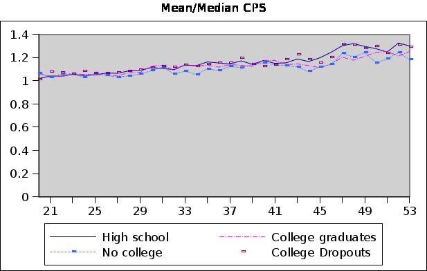
43 Figure A-2: Statistics by Education Groups: Data CPS 43