THE PROPOSITION VALUE OF CORPORATE RATINGS - A RELIABILITY TESTING OF CORPORATE RATINGS BY APPLYING ROC AND CAP TECHNIQUES

Transcription

1 THE PROPOSITION VALUE OF CORPORATE RATINGS - A RELIABILITY TESTING OF CORPORATE RATINGS BY APPLYING ROC AND CAP TECHNIQUES LIS Bettina University of Mainz, Germany NEßLER Christian University of Mainz, Germany RETZMANN Jan Deutsche Pfandbriefbank, Germany Abstract: We analyze the Altman model, a Logit model as well as the KMV model in order to evaluate their performance. Therefore, we use a random sample of 132 US firms. We create a yearly and a quarterly sample set to construct a portfolio of defaulting and a counter portfolio of non-defaulting companies. As we stay close to the recommendations of the Basel Capital Accord framework in order to evaluate the models, we use Receiver Operating Characteristic (ROC) and Cumulative Accuracy Profile (CAP) techniques. We find that the Logit model outperforms the Altman as well as the KMV model. Furthermore, we find that the Altman model outperforms the KMV model, which is nearly as accurate as a random model. Keywords: Altman Model, Cumulative Accuracy Profile (CAP), Distance to Default, Logit Model, Moody s KMV, Receiver Operating Characteristic (ROC), Z-score. 1. Introduction For the second time in seven years, the bursting of a major asset - bubble has inflicted great damage on world financial markets. While reading economical newspapers, one could find phrases like the one from Stephen S. Roach (Morgan Stanley) in nearly every kind of newspaper. The past crisis found its starting point with defaulting US consumer credits and thus affected banks capital requirements immediately

2 The stock market reacted with massive price fluctuations. Especially bank and insurance titles got under enormous pressure. As a reaction, the European Central Bank (ECB) gave several short time credits to banks to secure liquidity. According to the Manager Magazine (2008), these credits amount to billion at the , billion at the and 300 billion at the The FAZ (2008) reported that the credit crisis causes a deceleration in economical growth especially in the US but in the EU as well. Was it possible to forecast the crisis? The President of the ECB Jean-Claude Trichet agreed to this opinion and blamed rating agencies to embellish the situation by giving overvalued rating grades to high risk financial products (FTD (2007)). To evaluate companies and financial products, rating agencies are using different kinds of rating models. Typically these models evaluate default risk by categorizing the company / the financial product in a predefined rating scale. In general, a rating grade is a synonym for a default probability forecasting a time horizon of one year. However, the procedure of how these models work is mostly unknown. In addition to commercial rating models, academic literature offers a huge range of publicly available rating models. The Z-score model by Altman (1968) for example, is probably the most known rating model. This model heralds an era of new valuation models, using statistics in order to measure and describe a company s probability of default. Up to date the model is used as a benchmark for every kind of credit risk model. To compensate disadvantages of Altman's linear model, academic literature describes a huge range of models using other, non linear techniques. Staying close to the present discussion about the performance of rating models, we analyze models which are applicable within the Basel framework. (Basel Committee on Banking Supervision (2001)). Therefore, the aim and objective of this paper is to figure out, whether the Z-score model, the bounded Logit model as well as the KMV model are appropriate systems to measure a company s default risk. Dealing with the various models performances, Engelmann et al. (2003) describe, that a rating system s quality results from its discriminate power to correctly distinguishing between non-defaulting firms and defaulting firms forward looking for a predefined time horizon. In order to test the rating models correctness, we apply the 'Cumulative Accuracy Profile Model' (CAP) and the 'Receiver Operating Characteristics Model' (ROC) techniques. According to Engelmann, both techniques are the most accepted evaluation techniques currently used in practice in order to analyze rating models performance. Due to the current developments and discussions regarding the regulation of rating agencies and the correspondent liability the analysis gets certain relevance (Eisen 2008). Applying these techniques, we find that the models differ in their forecast quality. Therefore, the Logit model outperforms the Altman as well as the KMV model. Furthermore, we find that the Altman model outperforms the KMV model. The results give helpful suggestions for understanding the models and the arrangement of the regulative institutions

3 2. Model review The literature and academic examination regarding credit risk modeling has increased immensely since the source works of Altman (1968) and Merton (1974). Due to liberalization of capital markets, increases liquidity, completion on bond markets, developing and revisions of Basel Capital Accord Framework there is a grown practitioner s attentivements in correct credit risk assessment (Fernandes 2005). Structural models can be used for companies with equity or dept whichis traded on markets. In that case the approaches of Black/Scholes (1973) or Merton (1974) or the extension by Black/Cox (1976) or Longstaff/Schwarz (1993) can be used. By using valuation methods of option pricing theory, a credit facility is seen as a contingent claim on the value of the company`s assets. The default is defined to happen when the company hits the pre-defined default barrier. The Intensity models developed for e.g. by Jarrow/Turnbull (1995) or Duffie/Singleton (1997) do not try to measure the company s market value. The default is set to occur as the time of a first jump of a poisson process with random intensity. For companies which are not traded and no market based data is available, accounting related credit scoring models seem to be the common approach and following Allen (2002) seems to be the most effective and broadly accepted conceptualization (Fernandes 2005). The credit scoring approach was discussed intensively in academic literature since Beaver (1966) and Altman (1968). Barniv/McDonald (1999) state in a meta-analytic study that in the Logit models were used or discussed 178 times between 1989 and 1996 and underline the popularity of the Logit Model. Saunders et al. (2002) describe that the Altman and the Logit model belong to the group of scoring systems. All scoring systems have in common that they use preidentified weighted factors to determine the probability of default. Altman (2002) refers to the Z-score model and the Logit model by writing that both models have in common, that they involve a set of financial indicators in combination with qualitative elements. Financial ratios therefore analyze firm s profitability, liquidity as well as its solvency in order to forecast its wealth. Ratios as well as weights result from empirical observations so that they best distinguish between bankrupt and non-bankrupt firms for an underlying dataset. The models differ in the way how they process these ratios. Whereas the Z-score model processes them in a linear way, the Logit model processes them in a Logit function. The KMV approach differs substantial as it is based on option theory. According to Navneet et al. (2005) the bankruptcy takes place, when the firm s market value of debt exceeds the firm s market value of equity. In that case the entrepreneur strikes and transfers the firm s assets to the bank. In the following the models in the analysis (Z-score Model, the Bounded Logit Model and the KMV Model) get a brief definition

4 2.1. The Z-score Model Altman s (1968) Z-score model forecasts corporate bankruptcy based on weighted financial ratios, processed in a linear function. Altman criticizes the inaccuracy of pure ratios analysis in order to evaluate companies default risk. He argues that especially size effects would deform the accuracy of ratios. The size effect explains that financial ratios deflate statistics by size. According to Altman, this is a particular problem if ratios are getting compared among different companies. In order to deal with the impact of size, Altman concentrates on multiple discriminate analyses (MDA). He defines the MDA approach as a statistical technique used to classify an observation into one of several a priori groupings dependent upon the observation s individual characteristics. It is used primarily to classify and / or make predictions in problems where the dependent variable appears in qualitative form. Thus, the MDA analysis uses a mix of fixed ratios and combines them with fixed coefficients. The result is a value which should have enough explainable power to describe company s current and future performance. According to Altman the linear MDA function follows the form: Altman models the function with a relative small number of selected measurements. The underlying data set includes an overall sample size of 66 firms, splitted up into two sub groups consisting of 33 observations each. Whereas the first group includes firms following the characteristic non-bankrupt, the second group follows the characteristic bankrupt. Nonbankrupt firms are chosen on a random base under the limitation that they were active in the business field production and that they have an asset size between $1 and $25 million. This justification is done to minimize the size effect. The bankruptcy sample covers a time horizon from 1946 to All analyzed bankrupt firms were active in the business field production as well as under the partition of chapter seven of the National Bankruptcy Act (US). His sample size is due to a lack of data for bankrupt companies with an assets size less than million and a rare bankruptcy possibility of larger firms. Altman collects the bankruptcy data from financial statements published one period before the bankruptcy takes place. Using this data, Altman uses t-statistics in order to find, which ratios are appropriate in order to forecast a bankruptcy. Based on that, he develops weights for the financial ratios to distinguish between defaulting and non-defaulting companies. Therefore, the Z-score function is described as:

5 For the underlying data set he finds that companies with a Z-score less than 1.81 the default occurs within one year. In contrast, firms with a Z-score exceeding 2.99 are solvent within the next year. Altman describes that the best cut-off value falls between 2.67 and 2.68 so that he defines the ideal Z-score value as Applying the MDA function, Altman finds that it classifies 95% of all observations correctly. According to Richling et al. (2006), the model cannot be implemented into European solvency forecasts without changing the models weights. This is due to different accounting stands between the US and the EU Bounded Logit Model In comparison to the linear Z-score model, the bounded Logit model uses nonlinear techniques to compute the probability of default. Therefore, the models procedure is as follows; a firm can either go bankrupt or stay healthy, which can be described as for a bankrupt firm and for a non-bankrupt firm. The models probability that x is a defaulting company of the function i x can be described as:

6 The model aims to estimate. Therefore Cramer (2007) describes that the probability that a bankrupt firm is in a random sample follows the Bayes rule, which can be expressed as: According to Cramer, formula four can get maximized in order to find a correct decision. Therefore he describes, that if the fraction of non-defaulting firms is known, parameters of can be estimated from a given sample by using standard Maximum Likelihood methods. Using a sample size of 20,000 observations, Cramer finds the standard bonded model to forecast a firm s health best. Its main advantage against the standard Logit models is that its upper bound decreases the influence of outliners. The standard bounded Logit model follows the form: Using binary dependent variables, the bounded Logit model estimates default probabilities relative to a cut-off value. Comparing the MDA approach to the Logit model, Tang (2006) describes the Logit models advantage over the MDA method is, that it does not assume multivariate normality. Whereas both models have in common that they use weighted ratios as input variables. Cramer defines the approach as an analysis that links the probability of a firm going bankrupt to its initial ratios. Like Altman, Cramer defines ratios as well as weights for his function, by analyzing which ratio in combination with which weight is most appropriated, to distinguish between defaulting and non-defaulting firms in the underlying data set. Therefore, the bounded Logit model transfers the input data into a nonlinear form whereas its upper bound is 1.1. According to Cramer the upper bound reduces the impact of outlines in the rating results. Using his data set, he estimates the upper bound as a best practice value such that it fits the data base best. Therefore, Cramer defines the bounded Logit model as:

7 Applying this Logit function, the cut-off value lies according to Cramer between 0.03 and 0.1. Whereas values above 0.1 explain, that the company will not default during the next year. A rating outcome under 0.03 describes a high probability that a bankruptcy occurs within the next year The KMV Model More recent models differ substantially from the Z-score and the Logit approach. Wahrenburg et al. (2000) describe that two different approaches are dominating the academical as well as practical world nowadays. These two approaches are: Asset-value-models and Loss-rate-models As this paper focuses on linear, Logit and as well as asset value models, the loss rate approach will not be discussed and is just mentioned in sense of completeness. Asset-value-models are based on option model theory. As Moody s assetvalue-model has a major impact on the rating market, we test its reliability. The KMV Model has been developed by KMV Corporation in 1988 and got sold to Moody s Corporation in 2002 (Moody s presents and promotes the model under In this approach, the entrepreneur has an interest to liquidate the company if the market value of the firms debt is higher than the market value of its equity. Following Sreedhar/Shumway (2004) the model computes this event by subtracting the face value of the firm s debt from an estimated market value of the firm and then divides this difference by an estimated value of the firm s volatility. This procedure results in a Z-score value, which is expressed as the distance to default

8 (DD). In order to estimate whether the face value of a firm s debt is higher than the market value of its equity, the DD gets substituted into a density function. To compensate the lack of unknown variables in the density function we use Sheedhar s naïve version of the KMV model. Sheedhar develops naïve probabilities to estimate the DD. Starting to measure a firm s market value, he assumes that the firm s market value equals the sum of its market value of debt and market value of equity. In order to estimate the market value of debt, the model sets the book value of debt equal to the market value of debt, which is defined as: Furthermore, he assumes: that a company which is close to default has risky debt and that this risky debt correlates with risky equity. Using this correlation the debt s volatility is assumed to be: According to Sreedhar, the five percent value in equation eight represents the term structure of volatility times the equity volatility gets included to embrace the volatility associated with default risk. Combining equation seven and eight, Sreedhar describes the firms overall volatility as: After computing the overall volatility, the companies expected return on assets equals the firm s stock returns over the previous year, which gets expressed as;

9 According to Sreedhar combining equations nine and ten, the DD gets computed as: Furthermore, Sreedhar (2004) describes that the stock market data needs to be adjusted by the return of the firm in year t-1 minus the value-weighted S&P 500 / S&P t-1 ( - ). As it is our aim to test models which are adaptable in the Basel Accord framework, the naïve version estimated DD s have to be as close as possible to the results estimated by the original KMV model. Sreedhar therefore mentions, that the naïve version keeps the structure of the KMV Model in terms of its DD as well as the expected default frequency without solving equations simultaneously. Furthermore, the model includes nearly the same quantity of information as the original KMV model, except of the underlying distribution and the market value of the firm s assets. According to Saudners et al. (2002), especially the underlying distribution highly influences the estimated DD. To bridge the unknown distribution function KMV applies, the naïve version assumes the underlying default function to be normally distributed. Furthermore, critical inputs used by the naïve version are the face value of equity and thus the equities volatility as the time horizon of the analyzed equity returns only covers one year. Sheedhar explicitly mentions that the model links the firm s equity value to a default event such that a declining equity value implies an increasing probability of default. Comparing this approach with the Z-score and the bounded Logit approach, the naïve KMV model reacts in the moment of declining share prices by scaling down the DD. The other two models require mainly balance sheet data, which gets published on a quarterly base. After computing the naïve KMV model and comparing the outcome with public available rating outcomes from KMV, Sreedhar concludes that the naïve KMV model has predictive power for default forecasts, whereas the models main strength is based on its functional form rather than from solving the two nonlinear equations

10 3. Methodology By their very own nature, rating models can be erroneous. Applying statistical tests in order to analyze ratings accuracy, Satchel et al. (2006) describe that any rating model needs to identify defaulting obligators from non-defaulting operators within a predefined time horizon better than a random model would do it. According to Beling et al. (2005) the models cut-off value therefore plays a crucial role in order to get an appropriate performance forecast. The cut-off value acts as a decision maker to classify an obligator. Altman's cut-off value for example is Thus, if the Z-score model and its cut-off value are appropriate, it has to determine non-defaulting obligators and defaulting obligators with a higher likelihood as a random model would do it. The situation, in which a rating system does not perfectly reflect reality, is described in graph I. The graph shows a distribution of defaulters as well as a distribution for non-defaulters. If the rating would perfectly distinguish between defaulting and non-defaulting firms in respect to the cut-off value, the two distributions would not overlap each other. Line C labels the models cut-off value. If misevaluation takes place, two different types of errors can occur. Spuriously a company gets evaluated as a default candidate whereas the firm is healthy. Alternatively the firm could get misleadingly evaluated as a healthy one. Taking errors and correct decisions into account, table I presents all possible rating outcomes

11 Blöchlinger et al. (2005) describes, that an alpha error occurs if the model estimates a lower risk as it is given. In contrast, the beta error describes, that the model estimates a company at a higher risk level as it is given in reality. In order to test ratings whether they reflect reality in a way which is sufficient to determine company s economical robustness, the Basel Committee on Banking Supervision (BCBS) (2000) published several approaches achieving these requirements. According to the BCBS, ROC and CAP curve approaches are an appropriate statistical measure to test rating accuracy. Satchell et al. (2006) refer to the BCBS (1999) by writing, that both methods are popular measurements to evaluate a rating models performance in practice. As an advantage of the ROC and CAP techniques against other performance measurements, Blöchlinger points their ability to visualize a systems performance. Therefore, the ROC and CAP graphs label the coordinate axis with hit and false rate The ROC curve The ROC curve is defined by Blöchlinger et al. (2005) to be a two dimensional measure of classification performance and visualizes the information from the Kolmogorov Smirnov statistics. According to Engelmann et al. (2003) the ROC is computed by using the percentage of defaulters whose rating scores are equal or lower than the maximum score fraction of the overall sample size. Thus, the systems correctness is getting measured by using the total number of observations and the fraction of observations the system incorrectly assigns as non-defaulters. Starting with non-defaulters, their fraction is mathematically measured and expressed in terms of the hit-rate. According to Blöchlinger the hit-rate is described to be one minus the alpha error under the null hypothesis that high scores are translated into high default probabilities. Therefore, the hit rate gets expressed as: Thus, this measure describes the number of defaulting firms found correctly in the sample. After estimating the number of defaulters found correctly in the sample, the amount of defaulters that were classified erroneously has to be identified. In order to do so, the false alarm rate has to get computed. According to Satchel et al. (2006), the false alarm rate is defined to be the number of non-defaulters that were classified

12 incorrectly as defaulters by using the cut-off value. Thus the false alarm rate measures the beta error. The rate is defined as: To illustrate that, we apply the HR and FAR methodology at the Altman (1968) paper. According to Altman (1968), the Z-score model has a targeting precision of 95%. Thus for Altman s data set, the following numbers of correct and incorrect observations are described: Therefore, the hit- and false alarm rates in respect to the cut-off value are: HR (2.675) = 31 / 33 = FAR (2.675) = 2 / 33 = The actual ROC curve now is estimated by using all possible cut-off values given by the model and combing them with the rating outcomes to compute the HR and FAR rate. We apply cut-off values according SPSS. The program starts by using one plus the highest rating grade given by a model and goes down in 0.05 steps to one minus the lowest rating grade given by a model. Going back to the Altman example, the fraction of bankrupt to non-bankrupt firms differs, if another cut-off value is set. Having these values, the HR and FAR differ as they analyze the fraction of defaulters to non-defaulters in respect to the actual cutoff point. The results are then plotted in a graph. Graph II illustrates that

13 As it can be seen from the graph II, the ROC curve s abscissa is labeled as false alarm rate and the ordinate labels the hit-rate. According to Satchel, a rating models performance is better the steeper the ROC curve is at its left end and the closer the curves position is to the point (0.1). Thus, a models performance can be measured in terms of the area under the curve the larger the area under the ROC the better the rating model. The area under the ROC (AUROC) is labeled as A in graph II. According to Hutchinson (2005) the ROC approach follows two hypothetical Gaussian distributions. Mathematically, the AUROC can be expressed as: As it is our aim and objective to find the rating system which offers the best performance in order to forecast bankruptcy, the decision rule is as follows: the system which produces the largest significant A value is the one with the best performance The CAP curve The CAP approach is alike the ROC approach. It is also used to measure the rating models performance. Instead of plotting the hit against the false rate like the ROC does it, the CAP uses the fraction of defaulters and plots it against the fraction of all obligators. Satchell et al. (2006) define the CAP techniques as: for a given fraction x of the total number of debtors the CAP curve is constructed by calculating the percentage d(x) of the defaulters whose rating scores are equal to or lower than the maximum score of fraction x. Graphically, we described the CAP curve in Graph III

14 In order to apply the CAP, the rating outcomes have to be rearranged first. Therefore, the outcomes have to be ordered from the safest to the most risky obligator. A perfect rating model would allocate the lowest rating grade to the firm which is most likely to go bankrupt and the highest rating grade to the safest firm in the defined time horizon. In this case, the model would reflect reality perfectly and the CAP curve would go straight to the point (0.1) and stay at the line 1.1. In contrast, a random rating model is assumed to have no discriminate power. The random model is shown in graph III with the 45 degree line from point 0.0 to point 1.1. A real world rating scenario gives an output anywhere between a perfect and a random rating model. The random rating line plays a crucial role for the evaluation of a rating model with the CAP technique. Like the ROC, the CAP uses the area under the curve as an assessment factor. According to Fernandes (2005), in comparison to the ROC, the CAP does not use the whole area under the rating model curve, but the area between the random rating model and the rating model curve as an estimator for the models performance. This area is described as the Accuracy Ratio (AR) and is defined to be: Thus the decision rule for the CAP is; the larger the area between the random model curve and the rating model curve, the better the model describes reality. A perfect model therefore would be visualized in the graph as a horizontal line which crosses the point 1:1 in the coordination system. In order to represent a complete picture of the academical discussion linked to these two methodologies, Blockwitz et al. (2004) discusses problems of interpreting the ROC and CAP curves. Especially, the random model used in the CAP is critical in terms of describing the discriminate power of a model. Blockwitz focuses on the maximum value of one as a benchmark. Following their line of argumentation, this value would only occur, if all debtors are ranked correctly in relation to the random default event. This implies that after estimating a model results have to be ordered according to their value. Despite this critique, we use both models because the BCBS labels them as an appropriate tool to measure rating systems performances. 4. Data Every default model we analyze forecasts the default probability for a time horizon of one year. Thus, if a company gets bankrupt in 2007, any rating model

15 should evaluate the company as a default candidate with data from In order to test the models, we use the most recent and largest corporate bankruptcies between 2006 and 2008 in the US. We built two data sets, one with annual and one with quarterly data, which provides us in total with 132 observations. According to the sample size of the annual and quarterly data sets, we imitate Altman s (1968) approach. That gives us a sample size of 66 observations for each set, spitted in 33 observations following the characteristics bankrupt and 33 observations following the characteristic non-bankrupt. Starting to collect bankruptcy data, we us the database bankruptcydata.com. As a matter of particular interest, the page offers names of the 20 largest US bankruptcies of each year. Hereby, the authors do not distinguish, whether the company got under chapter seven or 11 of the US bankruptcy code. Using these companies as a starting point, we get balance sheets, income statements, cash flow statements, as well as stock market prices from Google-finance, Yahoo-finance, Data stream as well as the Securities and Exchange Commission (SEC) database. If it is not explicitly mentioned, the following paragraph does not distinguish between bankrupt and non-bankrupt companies. Especially the bounded Logit model and the KMV are models which are not restricted to a specific branch or business field. To test their broad applicability we collect data from firms, which are active in the following branches: Constructing companies (4), manufactures (8), energy production (2), telecommunication and information technology (5), retail industry (7), financial industry (5) as well as the airline industry (2). Furthermore, all companies have in common that they were / still are publicly traded. The accounting data provides all information to solve the bounded Logit model directly. In order to estimate the Altman model, the equity market value is estimated by multiplying the amount of outstanding shares times the stock market price at the announcement day of the annual / quarterly report. Data which is used to solve the KMV model differs substantially from data we use to

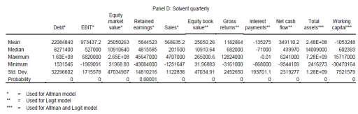
16 solve the Z-score and bounded Logit model. According to the models description, it is necessary to solve the following variables: volatility of stock returns, the face value of company s debt and the standard deviation of return. Stock market data to estimate the value of equity - formula nine and 11 - is gained from Google finance and Data stream. The numbers of outstanding shares are published within the company s balance sheets, downloadable at SEC. According to Sreedhar et al. (2002), we substitute the face value of a debt with the total amount of debt plus current liabilities published in the balance sheet. According to the relative short time horizon of our data set, we do not adjust the data from outliners. Using this data in order to compute the default probabilities, panels A D present descriptive statistics for the Altman and the Logit models. Panel I J include descriptive statistics for the KMV model. The structure is as follows; first we present the insolvent yearly data and the solvent yearly data. This is followed by the insolvent quarterly and the insolvent yearly data description. Facing Panel A and B we find that insolvent firm s have less debt than solvent firms. The higher standard deviation in the insolvent set indicates that debt is more dispersed for insolvent firms than for solvent firms. The EBIT draws a clear picture between solvent and insolvent firms. Whereas insolvent firms have on average a negative EBIT, solvent firms show a positive one. Comparing the EBIT maximum values, the insolvent data set shows still a positive value, but compared to the solvent sample it is more than 10.5 times lower. The market value of equity equals outstanding shares times the stock market price both collected at the announcement day of the annual reports. Whereas the insolvent data set clearly indicates that the market evaluates defaulting firms low, the values of the solvent firms are highly dispersed among the sample. Thus, it seems reasonable, that the insolvent maximum value is by far lower than the minimum value of the solvent data set. As the solvent firms EBIT value is higher than the one of insolvent firms, it seems realistic that retained earnings of insolvent firms are lower than retained earnings of solvent firms. On the other hand we observe that the insolvent values are not that dispersed among the sample as they are in the solvent data set. Interesting to observe is, that insolvent firms do have much better sales values than solvent firms. Even though the insolvent data set shows a much higher standard deviation, both, the maximum as well as minimum values are higher than the comparable values in the solvent data set. Facing the equity book values, we also find that insolvent firms have higher equity book values than solvent firms have. Whereas both standard deviation values are very high, the one of the insolvent set is much higher than the solvent one. In terms of gross returns, insolvent statistics are showing values far below the solvent values, whereas the solvent data set shows a higher standard deviation. As it can be assumed from the different debt levels, insolvent firms have less interest payments than solvent firms. Remarkable for both samples is the negative net cash flow whereas the solvent samples standard deviation is higher

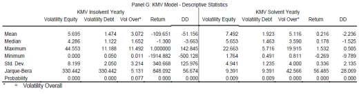
17 Both, total assets as well as working capital are used to estimate the Altman as well as the Logit model. Insolvent firms have on average less total assets and show a lower standard deviation than the solvent firms. Facing working capital we find that insolvent firms have on average more working capital than solvent firms. Furthermore, they show a higher standard deviation. Turning the view to the quarterly data set we get comparable results as we get them for the yearly data set. Therefore, we focus on differences between the yearly and the quarterly data set. Descriptive statistics of the quarterly set are presented in Panels C D. While the yearly set shows on average a positive EBIT for insolvent as well as for solvent firms, the quarterly set shows a highly negative EBIT mean for insolvent firms. Furthermore, interest payments of insolvent firms doubled for the annual data in comparison to the quarterly data set. Moreover, firms in the solvent sample generate a positive net cash flow whereas insolvent firms generate a much lower net cash flow than they do it in the annual sample. On the other hand, solvent firms show a negative mean of working capital what differs to insolvent firms, which are generating a positive working capital on average. While presenting these results, it is worth to mention that in ten times, the last annual reports were closer to the default event than the last quarterly report were. Furthermore, we find that banks have a massive impact on the statistics presented. Descriptive statistics of the KMV model are presented in Panel G and J. We find that insolvent firms show lower equity volatility than solvent firms. Furthermore, insolvent firms have a lower debt volatility than solvent firms. In all samples, the debt volatility on average has a value between 0.59 and Also interpreting mean values, we find that the overallvolatility differs among the samples with value between 8.15 and 1.6., so that solvent firms have compared to insolvent firms higher values. In terms of returns, we find that insolvent firms have on average highly negative values whereas we find for solvent positive returns on average

18 - 77 -

19 - 78 -

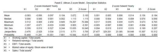
20 5. Results As it can be assumed while reading the models descriptive statistics, the three different models show an inhomogeneous performance. Whereas the performance varies among the different models it also differs among the data sets. While presenting the results we keep the structure used in the parts above, so that we first present the Altman model, which is followed by the Logit and the KMV model. After presenting descriptive statistics of the models results, we do not distinguish anymore between the solvent and insolvent data set but use the full data set to analyze the models performance. Descriptive statistics are followed by analyzes of alpha and beta errors. The evaluation is concluded by presenting the ROC and CAP results. As it can be seen from Panel E, the yearly Z-score values for insolvent companies differ quite a lot among the sample. Whereas the mean is about 5.18, the minimum value is around and the maximum value is about Thus, according to the cut-off value of 2.675, we can assume that the model forecasts insolvent firms mainly incorrect. Furthermore, it is conspicuous that the standard deviation has, compared to the other models, the highest value with The solvent data Z-scores differ sustainably from the insolvent Z-scores. Here, the mean is around times lower as what we observe in the insolvent data set. Furthermore, both the maximum as well as the minimum values are below zero. Linking the values to the cut-off value, we find that the model cannot correctly forecast this sample. Coming to the yearly Logit model in Panel F, the statistics are painting another picture. Reminder; the model has an upper bound, means that the maximum values cannot extent 1.1. The insolvents set maximum value is close to the upper bound but does not reach it, as it has a value of With a minimum value of zero, the model reaches a standard deviation of 0.195, which is compared to the other models the lowest value in the sample. Thus, we can confirm Cramer s (2007) observation, that the bounded Logit model reduced the occurrence of outliners. According to the cut-off value of 0.1, we find that the model evaluates defaulting firms mostly incorrect. The counter sample produces higher maximum as well as minimum values as the insolvent data produces. The maximum value reaches the models upper bound. Furthermore, the mean equals

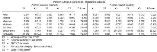
21 0.73. According to the cut-off value we can assume that the model forecasts solvent firms mainly correctly. Coming to the KMV models distance to default value in Panel G, we find highly dispersed values for the insolvent data set. As the standard deviation exceeds 125, the model generated the highest value in the sample. With a mean of a maximum value of and a minimum value of -500,128 we assume that the model forecasts the dominating amount of defaulting firms correctly. This picture changes by facing the solvent data. Here, the model generates values close to zero or even negative. With a maximum value of 0.5 and a minimum value of -9.7 the model generates a standard deviation about Combining that with a negative mean value, we can assume that the model forecasts solvent firms mainly incorrect. Furthermore, for both samples, the model generates a distribution, which is not normally distributed. Compared to the yearly data set, the quarterly data shows differences. The Altman model, presented in Panel H, estimates a maximum value of 74.05, a minimum value of -0.81, with a standard deviation of Having a mean value of and the cut-off value of we get low evidence to presuppose in which direction the model could forecast firms. However, the mean gives evidence to assume that the model could forecast defaulting firms incorrectly. Estimations with solvent data generating values close to one. With a very low standard deviation of and a mean of we can assume the model to forecast defaulting firms mainly incorrect. The Logit s insolvent estimations in Panel I show a maximum value equal to the models upper bound and a minimum value of zero. As the standard deviation is around 0.25 and the mean is 0.57 we assume the model having problems to find defaulting firms. For the quarterly data, the model generates the same maximum and minimum value as it generates them with the yearly data, but reaches a higher standard deviation of 0.41, as well as a higher mean of According to the cut-off value we can assume that the model mainly forecasts solvent firms correct. Coming to the KMV quarterly results in Panel J, we find that that the model reaches a very high maximum value in combination with a relative small minimum value. As the standard deviation is also very high we can assume that the model generates outlines which are influencing the statistics. The solvent data differs. Here, the values are relatively small as the maximum equals and the minimum equals , the model generates a standard deviation of 4.4. Having a mean of 1.59 we can assume that the model finds solvent firms better than it finds insolvent firms. Furthermore, the model does not generate a normal distribution, which is in the version we are using, a fundamental underlying assumption Alpha / Beta errors Remembering that the alpha error describes that even though the rating outcome forecasts no bankruptcy, the firm defaults. In comparison, a beta error

22 explains that a rating assumes a firm to go bankrupt which is not the case in reality. Table III therefore summarizes our rating outcomes categorized into correct decisions and alpha and beta errors. As one probably presumes by reading the descriptive statistics, the Altman models performance is, in terms of the beta error and its correct decisions low. We find the alpha error six and the beta error 33 times. The model assumes every company in the solvent data set to be bankrupt. In total, the model does 27 correct decisions. Whereas its strength is to correctly find defaulting firms. Thus, out of 66 observations, the Altman model categorizes 40.9% of all firms correctly. Interestingly, the model shows another performance for the quarterly data set. The alpha error decreases to one observation and the beta error stays constant at 33 observations. In total, 32 correct decisions are done. Out of the solvent data set, the model assumes no company to be solvent next year. Furthermore, it does 33 correct decisions by finding bankrupt companies. Thus, the Altman model evaluates 48.48% for the firms in the quarterly data set correctly. Noticeable for both data sets is that the model has a very high beta error and thus, it evaluates every solvent company incorrectly. Coming to the yearly Logit model, it is obvious that it has problems identifying bankrupt candidates. As table III shows, the model produces 32 alpha errors. In comparison, the beta error is very low with a total of three observations. In sum, it does 31 right decisions, whereas it only has two correct observations in terms of an actual bankruptcy, so that it evaluates 28 firms correctly. Thus, the model finds in 46.96% of all observation the correct decision. The results changes slightly by analyzing the quarterly data set. Here, we observe an alpha error of 31 and a beta error of five observations. In 30 times the model finds the right forecast. Out of the 30 correct decisions it only forecasts two bankrupt firms properly. Thus, the model finds 45.45% of the firms in the data set correctly

23 In comparison to the Altman model, which mainly forecasts default candidates correctly, the Logit model has a very high alpha error. Therefore, we summarize that the Logit model forecast defaulting firms mostly wrong, but forecasts non-bankrupt firms with a higher probability than the Altman model does it. Below the Altman and the Logit model, table III presents alpha and beta errors done by the KMV model. Reminder, compared to the Altman and the Logit model, the KMV model is the only one, which is based on option pricing theory. Facing the yearly data set, the KMV model does the alpha error six and the beta error 32 times. In total, it finds 28 times the right decision, whereas it evaluates only one non-defaulting company correctly. Thus is does in times the correct decision. The picture changes by coming to the quarterly KMV outcomes. Whereas we find 12 alpha errors, the beta error occurs 11 times. The total amount of correct decisions is 43. Thus, the KMV model finds in 65.15% of all observations the correct decision. Interesting to observe is that the models performances differs quit a lot. Whereas it shows a hit rate of 42.42% for the yearly model, the performance for the quarterly data set is about 29.24% better. Even if these results do not give an interpretable outcome in terms of the Basel Accord framework, they indicate that all three rating models could have to high false rates. To do further analysis we now present the ROC and CAP estimations ROC results While discussing the ROC curve and its AUROC, the decision rule is as follows. The larger the area under the curve the better is the ratings performance. Therefore, a value of one indicates, that the model has the highest possible explanatory power. A value of zero indicates that the model has no explanatory power. In a real world scenario, the models performance should be anywhere between zero and one. Reminder; by estimating the ROC, the program changes the cut-off values the get different hit- and false alarm rates. Therefore, it starts with one plus the highest rating grade as a cut-off value and goes down in 0.05 steps till one minus the lowest rating grade. Exemplary, we estimate the hit- false alarm rate with the models original cut-off values in table IV

24 In the ROC graphs presented below, the 45 degree line labels a random models performance, the curve labels the ROC estimations. The significance values are based on a 95% confidence interval. Graph IV shows the Altman models ROC estimations for both data sets. Both curves are created with 33 defaulting and 33 non-defaulting companies. The estimates are presented in table V. Altman s yearly AUROC equals Furthermore, it generates a significance value of Thus, the Altman model has an explanatory power of in terms of the significance value. The models explanatory power slightly improves by analyzing the quarterly data set. Here, the significance value equals 0.04 whereas the AUROC stays constant at Furthermore, the upper bounds level stays dominate at a nearly constant level. Summarizing the Altman model for both data sets by applying ROC techniques, we find that the models power for both samples is close to each other, whereas both models fulfill the requirements of the ROC to be better than a random model

25 Next, we test the Logit model. As it can be seen on the left side of graph V - the yearly sample - a major part of the ROC curve, except of the curves upper right corner, is above the random models line. Therefore, table VI.I shows, that the AUROCs value is As the significance value is above 0.05 the model has less explanatory power. Furthermore, the curve has a dominating upper bound. Looking at the right part of graph V we see that the ROC curve is highly above the random line. Only at the upper right part the curve is under the random models line. Table VI.II. presents the test results. As it can be seen, the AUROC equals 0.83 and the model produces a significance value of zero which proofs, that the model performs better than the random model does it. In comparison to the Altman and Logit model, the KMV model performs badly. It s clearly visible from Graph V.I that the yearly estimations performing worse than a random model would do it. Therefore, we estimate an AUROC value of The models significance value is 0.01 and thus it describes that the model has explanatory power

26 The quarterly ROC curve is close to the random model line. Therefore, the model produces an AUROC value of Table VII.II shows the test estimations. We find a very high significant value of Based on that, the model is described to have no explanatory power. Summarizing the results based on the CAP estimations, we find that the Logit model performs best as it produces the highest significant AUROC value. The Logit model is followed by the Altman model, which generates two significant AUROC values. In comparison to the Logit model, both values are lower than the highest Logit AUROC. The KMV model performs worst; it generates the worst significant value and the smallest AUROC. After presenting the ROC estimations we apply further analyzes by employing CAP techniques CAP Results Our CAP estimations are based on a self made program. Even though the program is in line with comparable programs and computes the same test results, it does not provide a significance value as it was given for the ROC estimations. Therefore, the models evaluations are based on the integral between the random model and the CAP curve only. In all graphs, the line consisting of triangles ( ) labels the analyzed ratings. The line consisting of quadrates ( ) labels the perfect rating

27 model and the 45 degree line (-) labels a random rating outcome. Here, the decision rule is as follows; the larger the area between the analyzed models and the random models line, the better the rating. Graph VII displays the Altman models performances in terms of the CAP curve. The yearly sample produces a CAP curve which is, except of seven items in the upper right corner, mainly above the random models line. For the yearly data set, CAP estimations give a value of Therefore, the model performs better than the random model. In its right part, graph VII shows the quarterly CAP curve of the Altman model. The graph shows that 20 items are placed under the random models line. The CAP estimator equals 0,172. Therefore we can summarize that the Altman model produces a curve, which is mostly above the random ratings line. Furthermore we find differences between the two data sets. The CAP estimator of the yearly sample is 1.86 times higher than the estimator for the quarterly sample. Applying the same processes to the Logit model, we find a CAP value of for the yearly data set - Graph VIII shows the estimations. As it can be seen, 12 items are placed under the random models line. The quarterly data set generates a slightly better CAP value of Here four items are lying under the random models line

28 The KMV models performance, measured in terms of the CAP, is bad. As it is visible from Graph IX, the CAP curve for the yearly data set is far below the random model and thus, it generates a negative CAP value of The quarterly data set generates a CAP curve, which is loosely to the random model line. Therefore, it produces a value of , which is the lowest positive Cap value we measured. As it is our interest to find the best performing model, table VII summarizes the ROC and CAP results. Table seven provides information to determine the most accurate model. Therefore, the model with the highest significant ROC and CAP values is placed first. The model, which generates the second highest significant ROC as well as the second highest CAP, is classified at place two and so forth. If two models have either a higher significant Cap value or a higher CAP value they both are classified with same rank. As the models descriptive statistics and the analysis of alpha and beta errors already have shown, table VII concludes the picture that the models perform differently. Furthermore, we also observe differences between the yearly and the quarterly data set. Facing the ROC values, we find the Logit model to perform best as it produces the highest significant AUROC value in combination with the second highest CAP estimator. Thus, the Logit model is placed first. The Altman model also generates a significant AUROC value but compared to the Logit model the area under the curve is smaller, thus it takes place two. Rank three shows the Logit as well as the